HAL Id: insu-02867236
https://hal-insu.archives-ouvertes.fr/insu-02867236
Submitted on 16 Sep 2020
HAL is a multi-disciplinary open access
archive for the deposit and dissemination of
sci-entific research documents, whether they are
pub-lished or not. The documents may come from
teaching and research institutions in France or
abroad, or from public or private research centers.
L’archive ouverte pluridisciplinaire HAL, est
destinée au dépôt et à la diffusion de documents
scientifiques de niveau recherche, publiés ou non,
émanant des établissements d’enseignement et de
recherche français ou étrangers, des laboratoires
publics ou privés.
First detection of ozone in the mid-infrared at Mars:
implications for methane detection
Kevin Olsen, Franck Lefèvre, Franck Montmessin, Alexander Trokhimovskiy,
Lucio Baggio, Anna Fedorova , Juan Alday , Alexander Lomakin , Denis
Belyaev, Andrey Patrakeev, et al.
To cite this version:
Kevin Olsen, Franck Lefèvre, Franck Montmessin, Alexander Trokhimovskiy, Lucio Baggio, et al..
First detection of ozone in the mid-infrared at Mars: implications for methane detection. Astronomy
and Astrophysics - A&A, EDP Sciences, 2020, 639, pp.A141. �10.1051/0004-6361/202038125�.
�insu-02867236�
Astronomy
&
Astrophysics
https://doi.org/10.1051/0004-6361/202038125
© ESO 2020
First detection of ozone in the mid-infrared at Mars: implications
for methane detection
K. S. Olsen
1,2, F. Lefèvre
2, F. Montmessin
2, A. Trokhimovskiy
3, L. Baggio
2, A. Fedorova
3, J. Alday
1,
A. Lomakin
3,4, D. A. Belyaev
3, A. Patrakeev
3, A. Shakun
3, and O. Korablev
31 Department of Physics, University of Oxford, Oxford, UK
e-mail: [email protected]
2 Laboratoire Atmosphères, Milieux, Observations Spatiales (LATMOS/CNRS), Paris, France 3 Space Research Institute (IKI), Moscow, Russia
4 Moscow Institute of Physics and Technology, Moscow, Russian Federation
Received 8 April 2020 / Accepted 22 May 2020
ABSTRACT
Aims. The ExoMars Trace Gas Orbiter was sent to Mars in March 2016 to search for trace gases diagnostic of active geological or
biogenic processes.
Methods. We report the first observation of the spectral features of Martian ozone (O3) in the mid-infrared range using the
Atmo-spheric Chemistry Suite Mid-InfaRed (MIR) channel, a cross-dispersion spectrometer operating in solar occultation mode with the finest spectral resolution of any remote sensing mission to Mars.
Results. Observations of ozone were made at high northern latitudes (>65◦N) prior to the onset of the 2018 global dust storm
(Ls=163–193◦). During this fast transition phase between summer and winter ozone distribution, the O3volume mixing ratio observed
is 100–200 ppbv near 20 km. These amounts are consistent with past observations made at the edge of the southern polar vortex in the ultraviolet range. The observed spectral signature of ozone at 3000–3060 cm−1directly overlaps with the spectral range of the methane
(CH4) ν3vibration-rotation band, and it, along with a newly discovered CO2band in the same region, may interfere with measurements
of methane abundance.
Key words. planets and satellites: atmospheres – planets and satellites: composition – planets and satellites: detection – planets and satellites: terrestrial planets – radiative transfer
1. Introduction
Ozone (O3) on Mars was first observed by the Ultraviolet
Spec-trometers on Mariner 7 and 9 (Barth et al. 1973;Barth & Hord 1971), which showed large variability and established seasonal trends. Since then, O3has been observed by ground-based
cam-paigns and spacecraft missions, but largely using absorption and emission features in the ultraviolet spectral range (e.g.Clancy et al. 2016;Perrier et al. 2006) or the thermal spectral range using the 9.7 µm band (Espenak et al. 1991;Fast et al. 2006). Here, we report the first observations of ozone absorption in the mid-infrared spectral region, between 3015 and 3050 cm−1, using the
mid-infrared channel of the Atmospheric Chemistry Suite (ACS) Mid-InfaRed (MIR) onboard the ExoMars Trace Gas Orbiter (TGO). This spectral region is shared by the ν3vibration-rotation
band of methane (CH4), as well as a newly discovered transition
of CO2 (Trokhimovskiy et al. 2020). The ability to
simultane-ously resolve these species has an impact on current and past attempts to measure the abundance of methane in the atmosphere of Mars.
ACS MIR is a novel cross-dispersion spectrometer making solar occultation observations of the limb of the Martian atmosphere. It has the finest spectral resolution of any Martian remote-sensing instrument to date, and the solar occultation technique provides a high signal-to-noise ratio (S/N), and strong sensitivity to the vertical structure of the atmosphere. These characteristics were instrumental in observing, for the first time, the mid-infrared 003←000 transitions of O3 in the atmosphere
of Mars.
Here we present solar occultation observations made in Mars year (MY) 34 by ACS MIR between solar longitude (Ls) 163–193◦ and north of 60◦N (May–June 2018). In this
region and time period, corresponding to the northern autumn equinox, we were able to observe significant amounts of ozone in the mid-infrared at altitudes below 30 km. In the following section, we describe the TGO mission, ACS instrument, and spectral fitting method. In Sect.3we present our observations, analysis, and comparison to model results and the literature. Section 4 discusses the implications that this observation has for CH4, which is sought in the same wavenumber range of the
infrared.
Ozone chemistry. The stability of the CO2 atmosphere on Mars depends on the abundances of odd hydrogen (H, OH, HO2),
which is a product of H2O photolysis. The primary source of O3
is a three-body reaction between O2 and O, while the primary
loss mechanism is the inverse reaction via photolysis. Such a cycle is neutral in terms of the quantity of odd oxygen remaining because O is converted to O3and vice versa. The main net-loss
pathway of the odd oxygen family Ox=O + O3 is the reaction
with HO2(HO2+O → OH + O2), which reduces Ox. Ozone is
therefore a valuable tracer of the odd hydrogen chemistry that stabilises the chemical composition of Mars’ atmosphere, as H, OH, or HO2have never been directly measured. Since odd
hydro-gen is primarily produced by H2O photolysis, ozone is expected
to be anti-correlated with water vapour (e.g.Clancy et al. 1996; Lefèvre & Krasnopolsky 2017;Perrier et al. 2006, and references therein).
A&A 639, A141 (2020)
The ozone profiles described here were all obtained at high northern latitudes around autumn equinox (Ls=160–190◦). At these latitudes and during this period, ultraviolet measurements performed in nadir geometry show ozone columns that rapidly increase with time (Clancy et al. 2016;Perrier et al. 2006). This dramatic rise in ozone occurs in conjunction with the buildup of the winter polar vortex and the quick decline in water vapour and O3-destroying odd hydrogen. Observations of the ozone
pro-file are sparse in the literature and do not cover the latitudes and local times sampled here. Indeed, almost all published profiles of ozone at high latitudes were measured later in the season, in the polar night (Gröller et al. 2018;Montmessin & Lefèvre 2013; Perrier et al. 2006). The only exceptions are the four polar ozone profiles measured by solar occultation in the ultraviolet range byPiccialli et al.(2019), but those were obtained in the south-ern hemisphere and at the edge of a fully developed polar vortex (Ls56–68◦). Our knowledge of the vertical distribution of ozone
is therefore still very limited, in particular in twilight conditions. However, all previous studies show that the largest ozone den-sities on Mars are always found in the polar vortices and that the polar ozone layer is usually located low in the atmosphere, typically between the surface and 20–25 km altitude.
2. Methods
The TGO was launched in 2016, began its nominal science phase in April 2018, and has completed 2 yr of observations at the time of publication. The primary scientific objectives of TGO are to detect any trace gases diagnostic of active geologic or biogenic activity, characterise and attempt to locate the possible sources of such trace gases, and characterise the water cycle on Mars (Vago et al. 2015). To achieve these goals, the TGO carries two suites of multi-channel spectrometers: ACS (Korablev et al. 2018), and the Nadir and Occultation for Mars Discovery (NOMAD;Vandaele et al. 2018). Both spectrometer suites have three channels and are capable of making observations in nadir, limb, and solar occultation viewing geometries.
The MIR channel of ACS is a cross-dispersion spectrometer consisting of a primary echelle grating, and a secondary grating used to separate diffraction orders (Korablev et al. 2018). The secondary grating rotates through several positions to access dif-ferent simultaneous spectral ranges. This work uses position 12, which covers the spectral range 2850–3250 cm−1that contains
the main CH4absorption band. This channel has the finest
spec-tral resolution (0.043–0.047 cm−1) of any atmospheric remote
sensing Mars mission and operates solely in solar occultation mode, benefiting from high signal strength, long optical path length, and the ability to directly probe vertical structure.
Calibration for these observations was performed at Russia’s Space Research Institute (IKI) and involves performing several corrections to the data before subtracting a dark signal from observations taken over a series of tangent altitudes and a solar reference measured above the top of the atmosphere. Transmis-sion spectra are obtained by dividing the corrected absorption spectra by the solar reference. Prior to transmission calculation, corrections applied to the data include removing dead or sat-urated pixels, accounting for subpixel drifts over time, and an ortho-rectification procedure needed to extract one-dimensional spectra from the two-dimensional detector array. See Fedorova et al.(2020),Olsen et al.(2020),Trokhimovskiy et al.(2020) for more details.
The instantaneous field of view (IFOV) of the instrument optics observing the edge of the solar disc is on the order of 1–4 km when projected at the Martian limb. The Sun edge is
imaged onto the detector array over approximately 15 rows, and from each row, a spectrum can be extracted. We use the intensity curve, which is a column of the detector array image and covers the vertical fields of view of each diffraction order (see Olsen et al. 2020), to identify a spectrum near the slit edge, which is closest to the centre of the solar disc.
Wavenumber calibration of each diffraction order is per-formed in two steps. An initial guess of wavenumber posi-tions for the solar reference spectrum is compared to the solar spectrum measured by the Atmospheric Chemistry Experiment Fourier Transform Spectrometer (ACE-FTS; Hase et al. 2010) in order to obtain a calibrated wavenumber vector. This is then refined using an appropriately clear transmission observation (avoiding signal attenuation due to aerosols) using transmis-sion lines from CO2, CO, or H2O, if they are available and of
sufficient strength.
Spectral fitting is performed by the Gas Fitting software suite (GFIT or GGG) maintained by NASA’s Jet Propulsion Labora-tory (e.g. Irion et al. 2002; Wunch et al. 2011). Over a given fitting window, volume absorption coefficients are computed for each gas and a spectrum is computed line-by-line. Non-linear Levenberg-Marquardt minimisation is done to determine a best-fit spectrum by modifying volume mixing ratio (VMR) scaling factors for a set of target gases. A set of estimated slant column abundances for all observed tangent altitudes is inverted with calculated slant column paths traced through the atmosphere using a linear equation solver to obtain a retrieved VMR vertical profile. Volume absorption coefficients are computed using the HITRAN 2016 line list (Gordon et al. 2017;Olsen et al. 2019), supplemented by H2O broadening parameters for a CO2-rich
atmosphere (Devi et al. 2017;Gamache et al. 2016).
The width of an instrument line shape is wavenumber depen-dent. Therefore, to obtain more accurate fits we use narrow fitting windows. The S/N of each spectrum, corresponding to a diffrac-tion order, is also highest in its centre due to the blaze funcdiffrac-tion of the echelle grating. To avoid errors in spectral calibration, we avoid working toward the edges of the spectra and cover the centre of each order with two or three windows that are 5– 6 cm−1 in width (a diffraction order in position 12 has a width
of 19–21 cm−1). There remains a curvature in the baseline of
the spectra. We use normalised spectra here and use an alpha shape, which finds the geometric area containing a spectrum, to estimate the baseline shape (Xu et al. 2019).
Accurate knowledge of temperature and pressure are critical for computing the number density of the atmosphere and per-forming accurate trace gas retrievals. In this work, temperature and pressure have been retrieved from observations of CO2lines
using coincident measurement made with the ACS near-infrared channel (Fedorova et al. 2020).
3. Observations and results
We first discovered the transmission signature of O3in ACS MIR
data during orbit 2476 (occultation N1), which was recorded on June 13 2018, or Ls=192.7◦. The local time was 17:16, and the
latitude and longitude of the tangent point were 66.5◦N, 13.5◦E.
This was shortly after the onset of the global dust storm of MY 34, which began around Ls=190◦ (Montabone et al. 2020), but
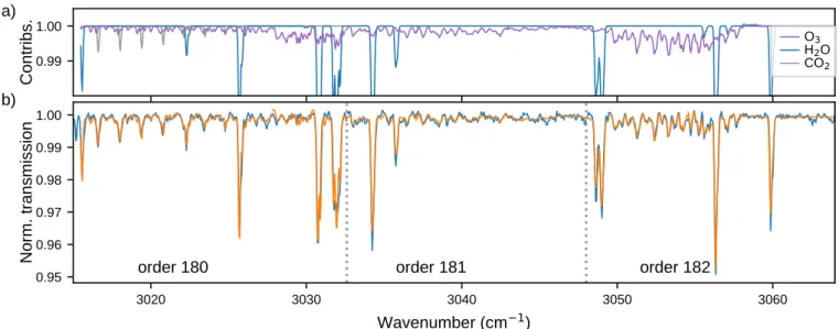
at such a high latitude that its impact was not yet felt and obser-vations with suitable transmittance were made down to 2.3 km above the aeroid. The signature was initially identified in order 182, covering the spectral range 3047.5–3067.5 cm−1, shown
in Fig. 1, with a computed best-fit spectrum. Once identified, the signature was also clearly identified in orders 180 and 181,
0.99
1.00
Contribs.
a)
O
3H
2O
CO
23020
3030
3040
3050
3060
Wavenumber (cm
1
)
0.95
0.96
0.97
0.98
0.99
1.00
Norm. transmission
order 180
order 181
order 182
b)
Fig. 1.Spectra recorded by ACS MIR at 5.5 km using secondary grating position 12 during occultation 2476 N1 on Ls=192.7◦: (a) contributions
from O3, H2O, and CO2to the best-fit for orders 180–182; (b) data and best-fits for orders 180–182.
0.975 1.000
N. trans.
17.98 km
0.975 1.000N. trans.
11.76 km
0.975 1.000N. trans.
8.63 km
0.95 1.00N. trans.
5.46 km
3020 3030 3040 3050 3060Wavenumber (cm
1
)
0.95 1.00N. trans.
2.28 km
Fig. 2.Same as Fig.1b, except at a range of altitudes.
shown in Fig.1b. The signature is very small relative to nearby H2O absorption lines and is only apparent in a small number
of observations, and at the lowest altitude levels. It is consis-tently visible over a range of observed tangent altitudes, and its evolution over altitude is also clearly distinguishable. Spectra from five consecutive tangent altitudes from the same occulta-tion are shown in Fig. 2, from the lowest observable tangent altitude of 2.3 km (which had a transmission level of 30%), up to 18 km, above which the signature vanishes in the instrument noise (we note there was a corrupt observation near 15 km). The CO2 lines towards the left side of order 180 in Figs. 1a, b are
not included in any current line lists and have been identified as a magnetic dipole absorption band of the 628 isotopologue of CO2; they are reported in a separate paper (Trokhimovskiy
et al. 2020) and the fit shown in Fig.1b uses line positions cal-culated in Trokhimovskiy et al.(2020), and line strengths and widths estimated from the nearby ν2+ ν3band of the16O12C18O
isotopologue of CO2. The spectral window covering this area
was not used to estimate the O3 abundance since the O3
transi-tions here are relatively weak and the CO2 spectroscopy is still
imprecise.
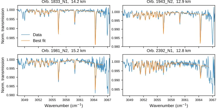
After the initial discovery, a careful search of all processed position 12 observations was undertaken. The signature was found in several other occultations, and often at higher altitudes. Figure3shows best fits in order 182 for four other occultations at altitudes near 15 km where the signature is strong and clear.
Figure4indicates where O3was identified over the evolution
A&A 639, A141 (2020) 0.985 0.990 0.995 1.000
Norm. transmission
Orb. 1833_N1, 14.2 km
Data
Best fit
0.980 0.985 0.990 0.995 1.000Orb. 1943_N2, 12.9 km
3049 3052 3055 3058 3061 3064 3067Wavenumber (cm
1
)
0.980 0.985 0.990 0.995 1.000Norm. transmission
Orb. 1981_N2, 15.2 km
3049 3052 3055 3058 3061 3064 3067Wavenumber (cm
1
)
0.985 0.990 0.995 1.000Orb. 2392_N1, 12.8 km
Fig. 3.Measured spectra and best-fits for order 182 for four occultations recorded between Ls=160–200◦and north of 65◦N.
200 250 300 350
Solar longitude L
s
( )
75 50 25 0 25 50 75 100La
tit
ud
e
(
)
Fig. 4.Latitudes of ACS MIR occultation tangent points as a function of
Ls. Dots in grey are ACS MIR occultations using grating positions other
than 12. Filled blue circles are full-frame observations, and empty blue circles are partial-frame observations. Occultations exhibiting strong O3
absorption features are indicated with arrows.
observations occurred early in the mission, and at high north-ern latitudes, greater than 60◦N and in the range Ls=160–200◦.
This is consistent with previous studies of the climatology of Martian O3that have reported accumulation over the poles
dur-ing fall/winter (Clancy et al. 2016;Perrier et al. 2006), resulting from reduced destruction pathways caused by low water vapour content and solar insolation. However, according to these stud-ies, the area of enhanced O3 should extend southward to 40◦N
and cover the time period Ls=180–360◦. We do not find
con-vincing signatures of O3 over the northern extent of ACS MIR
coverage in the range Ls=200–280◦ because of the onset of
the global dust storm. Indeed, the dust storm generally sets an
altitude limit on the vertical extent of solar occultation obser-vations of 25–35 km, below which meaningful signal is lost. In the range Ls=280–380◦, data volume constraints required us to
download only partial detector frames (open circles in Fig.4), which have not been fully processed.
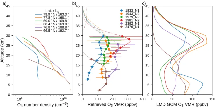
Vertical profiles of retrieved number densities and mixing ratios are shown in Figs.5a, b. The lower bound of the profiles indicates where the transmission signal dropped off to less than 0.05. The upper altitude limit, denoted by the transition from a solid to dotted line, indicates where the O3 absorption features
begin to be hidden in background noise, causing the retrieval uncertainty to grow larger than the VMR. The uncertainties shown in Fig.5b are the sum of the partial derivatives computed for the inversion of the matrices containing the number densities and slant paths (Jacobian matrix). In the right panel, Fig.5c, we also show vertical profiles generated by running the LMD gen-eral circulation model (GCM;Forget et al. 1999;Lefèvre et al. 2004) using a dust scenario for MY 34 (Montabone et al. 2020). Except for the earliest profile measured at Ls=163◦, all
pro-files indicate that the O3 density strongly increases at lower
altitudes. This suggests a gradual transition towards the sur-face O3layer typically observed in the winter polar vortex. The
largest O3densities reach 1010molec cm−3at 10 km and below, in
agreement with the polar profiles measured by the MEx SPectro-scopie pour l’Investigation des Caractéristiques Atmosphériques de Mars (SPICAM) in the southern hemisphere (Lebonnois et al. 2006;Montmessin & Lefèvre 2013).
SPICAM has also been used to measure the O3mixing ratio
near the south polar enhancement (Montmessin & Lefèvre 2013; Piccialli et al. 2019). These latter authors observed strongly increasing O3 abundance below 30 km toward 100–300 ppbv,
which was distinct from mid-latitude observations. These mix-ing ratios are comparable to those presented in Fig.5b, which are between 100 and 300 ppbv.
In Fig. 5c, the LMD GCM ozone profiles co-located with the ACS measurements also show a large variability in the short period of Ls sampled here. In general, the O3 mixing ratios
10
910
10O
3
number density (cm
3
)
0
5
10
15
20
25
30
35
40
45
Altitude (km)
a)
Lat. / L
s79.9 N / 163.3
77.8 N / 168.1
69.0 N / 169.8
68.4 N / 169.8
76.8 N / 188.8
66.5 N / 192.7
0
100
200
300
400
Retrieved O
3
VMR (ppbv)
0
5
10
15
20
25
30
35
40
45
b)
1833_N1
1943_N2
1979_N2
1981_N2
2392_N1
2476_N1
0
50
100
150
LMD GCM O
3
VMR (ppbv)
0
5
10
15
20
25
30
35
40
45
c)
Fig. 5.Panel a: retrieved number density or O3. Panel b: retrieved VMR vertical profiles of O3. Panel c: VMR vertical profiles of O3 extracted
from the LMD GCM at corresponding Ls, locations, and local times. Colours indicating occultation number are shared between panels.
calculated by the model are underestimated by almost of fac-tor of two relative to ACS MIR. This may reflect an imperfect timing in the model of the rapid decline in H2O that
accompa-nies the buildup of the northern polar vortex at this time of the year. Below 20 km, where ACS MIR observations are most sen-sitive, the model simulation shows a pronounced O3 minimum
for the earlier profiles (Ls=163–189◦) that is not seen in the measurements. The model outputs suggest that this problem is due to an overly strong poleward transport of H2O-rich air
origi-nating from mid-latitudes. The observation presented in Fig.5in brown, 2476 N1, is an outlier in that ozone decreases with alti-tude above 10 km. The other occultations from this period feature an increasing or roughly constant mixing ratio up to 30 km. In the LMD GCM, the shape of the O3profile for this latest
obser-vation (Ls=192.7◦) is also characterised by a strong decrease
above 20 km that contrasts with the earlier profiles. Examination of the model results shows that the change in the shape of this last O3profile is related to a large increase in H2O above 20 km,
which is also observed at the same time and location by the ACS NIR instrument (Fedorova et al. 2020).
4. Implications for CH4 observation
Ozone absorption below 30 km in the mid-infrared range has important implications for searches for atmospheric methane. Past observations of methane in the atmosphere of Mars (Formisano et al. 2004;Krasnopolsky et al. 2004;Mumma et al. 2009;Webster et al. 2015) were a driving cause of the develop-ment of the ExoMars TGO mission. CH4should have a relatively
short lifetime in the atmosphere of Mars (several hundred years), meaning current observations require an active source (Lefèvre & Forget 2009). A key objective of the TGO mission is to determine with certainty whether or not CH4 is present in the
atmosphere of Mars and what its spatial and temporal variabil-ity is, and to localise any possible sources. This story continues to be intriguing as the first results from TGO reported an upper limit on the order of 50 pptv (Korablev et al. 2019), and ACS
MIR observations continue to reveal no methane after one MY. In its place, we have instead found the rare and previously unde-tected signatures of O3 and a new CO2 magnetic dipole band
(Trokhimovskiy et al. 2020).
The strongest observed O3 features directly overlap
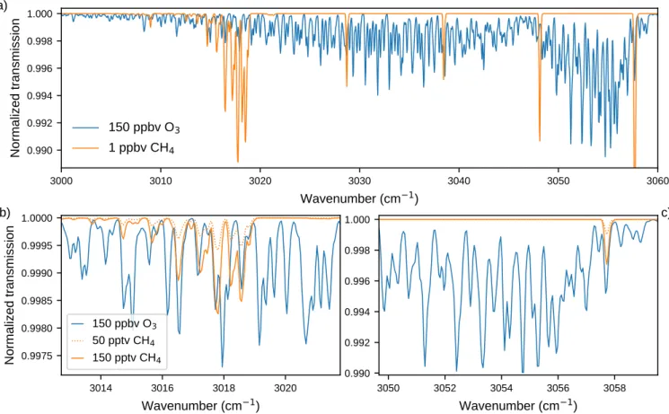
impor-tant methane features used by the Planetary Fourier Spectrom-eter (PFS) on Mars Express, the Tunable Laser SpectromSpectrom-eter (TLS) on Curiosity, and ground-based observatories. Figure6a compares the contributions to a transmission spectrum for 150 ppbv of O3 and 1 ppbv of methane. Figure 6b shows a
zoomed region surrounding the CH4 Q-branch, and Fig. 6c
shows a zoomed region surrounding the strongest line of the CH4
R-branch. Panels a and b also show 50–150 pptv of methane, approaching the upper limits reported by ACS (Korablev et al. 2019). In both cases, there is direct overlap between absorption lines of CH4and O3, with absorption lines produced by 150 ppbv
O3 being deeper than those from 150 pptv of CH4. Reported
values of methane abundance range from the background mea-sured by TLS of 0.4 ppbv (Webster et al. 2018) to enhancements measured by TLS and PFS of 6–16 ppbv (Giuranna et al. 2019; Webster et al. 2015). We computed model spectra at the reso-lutions of both instruments and are confident that errors can be made when CO2and O3spectroscopy is not accounted for.
The Q-branch is especially important for spectrometers with coarser spectral resolution than ACS MIR, as the integrated CH4 lines that make up the Q-branch would have a higher magnitude than the individual lines in the P- and R-branches. It would be observed in order 180 of ACS MIR, shown in Figs.1and2, and is located in the same spectral range in which we report previously unknown CO2 lines (Trokhimovskiy et al. 2020), identified in
Fig. 1a. The Q-branch is used by the PFS team in their CH4
analysis (Formisano et al. 2004;Giuranna et al. 2019), but with their spectral resolution, 1.3 cm−1, the entire Q-branch region is
integrated into only two or three spectral points.
The R-branch consists of a series of broadly spaced lines, the strongest of which lies at 3057.7 cm−1. This line has been
A&A 639, A141 (2020) 3000 3010 3020 3030 3040 3050 3060
Wavenumber (cm
1
)
0.990 0.992 0.994 0.996 0.998 1.000Normalized transmission
a)
150 ppbv O
3
1 ppbv CH
4
3014 3016 3018 3020Wavenumber (cm
1
)
0.9975 0.9980 0.9985 0.9990 0.9995 1.0000Normalized transmission
b)
150 ppbv O
350 pptv CH
4150 pptv CH
4 3050 3052 3054 3056 3058Wavenumber (cm
1
)
0.990 0.992 0.994 0.996 0.998 1.000c)
Fig. 6.Panel a: modelled transmission spectrum contributions from 150 ppbv of O3 and 1 ppbv of CH4. Panel b: close look at the modelled
contributions around the CH4Q-branch, but using 50 and 150 pptv of CH4. Panel c: close look at the modelled contributions around the strongest
line in the CH4R-branch.
resolution to observe the line as a triplet (Webster et al. 2015, 2018). The TLS instrument also has the capability to resolve the overlapping O3line as a triplet. At this resolution, one pair of O3
and CH4 triplet lines directly overlap (3057.685 cm−1), and the
other two pairs partially overlap. Despite this, the TLS team has not yet reported the abundance of ozone in Gale crater.
CO2 and O3 alone cannot account for the detections made
by both teams. In the case of PFS, the previously unknown CO2
features would impact all observations equally, as CO2is always
present and well-mixed. The PFS team has instead identified CH4 in only a small number of observations (Formisano et al.
2004;Giuranna et al. 2019). Furthermore, we computed spectra with O3at two and three times the quantities in our observations,
and the sheer magnitude of CH4observed by these latter authors
(15 ppbv) is far too large to be easily mistaken for O3.
In the case of TLS, which takes measurements of CH4at the
surface and mostly at night where and when the O3 abundance
is greatest, again, it is unlikely that the large quantity of CH4
observed (up to 9 ppbv) resulted from O3, yet the latter may
inter-fere in the measurement of the background level of methane in the so-called enriched mode as both ozone and methane should sustain the same enrichment.
For ground-based observations, strong O3 absorption
fea-tures from Earth’s atmosphere must first be removed before retrieving mixing ratios for Mars (Krasnopolsky 2012;Mumma et al. 2009); O3 must be accounted for, although this step
makes the retrieval more difficult (Zahnle et al. 2011). Finally, in the case of all previous observations, the rapid evolution and disappearance of CH4 are still not explained, although ozone
chemistry is very rapid, with a lifetime on the order of days.
5. Conclusion
The faint spectral signature of ozone, an established trace gas in the Martian atmosphere, has been observed for the first time in the MIR spectral region by the ACS MIR instrument on ExoMars TGO. These observations are limited to high northern latitudes (>65◦N) and prior to the onset of the 2018 Mars global dust
storm. During this time period, ACS MIR measurements pro-vide new insight into the vertical structure of ozone around the northern fall equinox and show the variability its VMR can have shortly before the polar vortex is established. We observe the dis-tinct presence of ozone with 100–200 ppbv at 20 km and below, which is close to the amounts measured in comparable condi-tions at the edge of the (southern) polar vortex. In general, the O3
mixing ratios retrieved by ACS MIR are higher than those calcu-lated by the LMD GCM. This seems to result from an overly wet atmosphere in the model at the time (equinox) and location (high northern latitudes) sampled here; these parameters will need to be confirmed in the future by simultaneous measurements of water vapour by ACS NIR.
We look forward to the processing of observations made in MY 35 and southern winter. Dust obscured the northern ACS observations after Ls190◦, but observations made after Ls∼ 30◦
in the next MY are very clear, and we expect to be able to detect low-altitude ozone near the southern hemisphere.
The observation of this trace gas at higher-than-predicted VMRs below 30 km has important implications for the detec-tion of methane in the atmosphere of Mars. This band, as well as the previously unidentified CO2 band, overlap and interfere
with the CH4 ν3 band used by TGO, MEx, and MSL to search
for methane. Accounting for these absorption features improves our own spectral fitting and will lead to more accurate lower lim-its in the future. In conclusion, our study shows that the O3lines
we report here interfere with measurements of Martian methane, but a detailed reanalysis of these measurements is required to precisely assess their impact.
Acknowledgements. The ACS investigation was developed by the Space Research Institute (IKI) in Moscow, and the Laboratoire Atmosphères, Milieux, Obser-vations Spatiales (LATMOS/CNRS) in Paris. The investigation was funded by Roscosmos, the National Centre for Space Studies of France (CNES) and the Ministry of Science and Education of Russia. The GGG software suite is main-tained at JPL (tccon-wiki.caltech.edu). This work was funded by the Natural Sciences and Engineering Research Council of Canada (NSERC) (PDF–516895– 2018), the UK Space Agency (ST/T002069/1) and the National Centre for Space Studies of France (CNES). All spectral fitting was performed by KSO using the GGG software suite. The interpretation of the results was done by K.S.O. and F.L. The processing of ACS spectra is done at IKI by A.T. and at LATMOS by L.B. Input and aid on spectral fitting were given by J.A., D.B., A.F., A.L., and F.M. The ACS instrument was designed, developed, and operated by A.P., A.S., A.T., F.M., and O.K.
References
Barth, C. A., & Hord, C. W. 1971,Science, 173, 197
Barth, C. A., Hord, C. W., Stewart, A. I., et al. 1973,Science, 179, 795 Clancy, R. T., Wolff, M. J., James, P. B., et al. 1996,J. Geophys. Res., 101, 12777 Clancy, T. R., Wolff, M. J., Lefèvre, F., et al. 2016,Icarus, 266, 112
Devi, V. M., Benner, D. C., Sung, K., et al. 2017,J. Quant. Spectr. Rad. Transf., 203, 158
Espenak, F., Mumma, M. J., Kostiuk, T., & Zipoy, D. 1991,Icarus, 92, 252 Fast, K., Kostiuk, T., Espenak, F., et al. 2006,Icarus, 181, 419
Fedorova, A. A., Montmessin, F., Korablev, O., et al. 2020,Science, 367, 297 Forget, F., Hourdin, F., Fournier, R., et al. 1999,J. Geophys. Res., 104, 24155 Formisano, V., Atreya, S., Encrenaz, T., Ignatiev, N., & Giuranna, M. 2004,
Science, 306, 1758
Gamache, R. R., Farese, M., & Renaud, C. L. 2016,J. Mol. Spectr.., 326, 144 Giuranna, M., Viscardy, S., Daerden, F., et al. 2019,Nat. Geosci., 1752
Gordon, I. E., Rothman, L. S., Hill, C., et al. 2017,J. Quant. Spectr. Rad. Transf., 203, 3
Gröller, H., Montmessin, F., Yelle, R. V., et al. 2018,J. Geophys. Res., 123, 1449
Hase, F., Wallace, L., McLeod, S. D., Harrison, J. J., & Bernath, P. F. 2010,J. Quant. Spectr. Rad. Transf., 111, 521
Irion, F. W., Gunson, M. R., Toon, G. C., et al. 2002,Appl. Opt., 41, 6968 Korablev, O., Montmessin, F., Trokhimovskiy, A., et al. 2018,Space Sci. Rev.,
214, 7
Korablev, O., Vandaele, A. C., Montmessin, F., et al. 2019,Nature, 568, 517 Krasnopolsky, V. A. 2012,Icarus, 217, 144
Krasnopolsky, V. A., Maillard, J. P., & Owen, T. C. 2004,Icarus, 172, 537 Lebonnois, S., Quémerais, E., Montmessin, F., et al. 2006,J. Geophys. Res., 111,
E09S05
Lefèvre, F., & Forget, F. 2009,Nature, 460, 720
Lefèvre, F., & Krasnopolsky, V. 2017, inThe Atmosphere and Climate of Mars, eds. R. M. Haberle, R. T. Clancy, F. Forget, M. D. Smith, & R. W. Zurek, Cambridge Planetary Science (Cambridge: Cambridge University Press), 405 Lefèvre, F., Lebonnois, S., Montmessin, F., & Forget, F. 2004,J. Geophys. Res.,
109, E07004
Montabone, L., Spiga, A., Kass, D., et al. 2020,J. Geophys. Res., 125 Montmessin, F., & Lefèvre, F. 2013,Nat. Geosci., 6, 930
Mumma, M. J., Villanueva, G. L., Novak, R. E., et al. 2009,Science, 323, 1041 Olsen, K. S., Boone, C. D., Toon, G. C., et al. 2019,J. Quant. Spectr. Rad. Transf.,
236, 106590
Olsen, K. S., Lefèvre, F., Montmessin, F., et al. 2020, Nat. Geosci., submitted Perrier, S., Bertaux, J. L., Lefèvre, F., et al. 2006,J. Geophys. Res., 111 Piccialli, A., Vandaele, A. C., Trompet, L., et al. 2019,Icarus, 113598
Trokhimovskiy, A., Perevalov, V., Korablev, O., et al. 2020, A&A, 639, A142
Vago, J., Witasse, O., Svedhem, H., et al. 2015,Sol. Syst. Res., 49, 518 Vandaele, A. C., Lopez-Moreno, J.-J., Patel, M. R., et al. 2018,Space Sci. Rev.,
214, 80
Webster, C. R., Mahaffy, P. R., Atreya, S. K., et al. 2015,Science, 347, 415 Webster, C. R., Mahaffy, P. R., Atreya, S. K., et al. 2018,Science, 360, 1093 Wunch, D., Toon, G. C., Blavier, J. L., et al. 2011,Phil. Trans. R. Soc. A, 369,
2087
Xu, X., Cisewski-Kehe, J., Davis, A. B., Fischer, D. A., & Brewer, J. M. 2019, AJ, 157, 243