The X-shooter Spectral Library (XSL): Data release 2

HAL Id: hal-03152017

https://hal.archives-ouvertes.fr/hal-03152017

Submitted on 28 Feb 2021

HAL is a multi-disciplinary open access

archive for the deposit and dissemination of

sci-entific research documents, whether they are

pub-lished or not. The documents may come from

teaching and research institutions in France or

abroad, or from public or private research centers.

L’archive ouverte pluridisciplinaire HAL, est

destinée au dépôt et à la diffusion de documents

scientifiques de niveau recherche, publiés ou non,

émanant des établissements d’enseignement et de

recherche français ou étrangers, des laboratoires

publics ou privés.

The X-shooter Spectral Library (XSL): Data release 2

A. Gonneau, M. Lyubenova, A. Lançon, S. Trager, R. Peletier, A. Arentsen,

Y.-P. Chen, P. Coelho, M. Dries, J. Falcón-Barroso, et al.

To cite this version:

A. Gonneau, M. Lyubenova, A. Lançon, S. Trager, R. Peletier, et al.. The X-shooter Spectral Library

(XSL): Data release 2. Astronomy and Astrophysics - A&A, EDP Sciences, 2020, 634, pp.A133.

�10.1051/0004-6361/201936825�. �hal-03152017�

https://doi.org/10.1051/0004-6361/201936825 c ESO 2020

Astronomy

&

Astrophysics

The X-shooter Spectral Library (XSL): Data release 2

?

,

??

A. Gonneau

, M. Lyubenova

, A. Lançon

, S. C. Trager

, R. F. Peletier

, A. Arentsen

, Y.-P. Chen

,

P. R. T. Coelho

, M. Dries

, J. Falcón-Barroso

, P. Prugniel

, P. Sánchez-Blázquez

, A. Vazdekis

, and K. Verro

1 _{Institute of Astronomy, University of Cambridge, Madingley Road, Cambridge CB3 0HA, UK} e-mail: agonneau@ast.cam.ac.uk

2 _{Kapteyn Astronomical Institute, University of Groningen, Landleven 12, 9747 AD Groningen, The Netherlands} 3 _{ESO, Karl-Schwarzschild-Str. 2, 85748 Garching bei München, Germany}

4 _{Observatoire Astronomique de Strasbourg, Université de Strasbourg, CNRS, UMR 7550, 11 rue de l’Université, 67000 Strasbourg,} France

5 _{CRAL-Observatoire de Lyon, Université de Lyon, Lyon I, CNRS, UMR 5574, Lyon, France}

6 _{New York University Abu Dhabi, PO Box 129188, Abu Dhabi, UAE}

7 _{Leibniz-Institut für Astrophysik Potsdam (AIP), An der Sternwarte 16, 14482 Potsdam, Germany} 8 _{Instituto de Astrofísica de Canarias, Vía Láctea s/n, La Laguna, Tenerife, Spain}

9 _{Departamento de Astrofísica, Universidad de La Laguna, 38205 La Laguna, Tenerife, Spain} 10 _{Departamento de Física de la Tierra y Astrofísica, UCM, 28040 Madrid, Spain}

11 _{Universidade de São Paulo, Instituto de Astronomia, Geofísica e Ciências Atmosféricas, Rua do Matão 1226,} 05508-090 São Paulo, Brazil

Received 1 October 2019/ Accepted 29 December 2019

ABSTRACT

We present the second data release (DR2) of the X-shooter Spectral Library (XSL), which contains all the spectra obtained over the six semesters of that program. This release supersedes our first data release from Chen et al. (2014, A&A, 565, A117), with a larger number of spectra (813 observations of 666 stars) and with a more extended wavelength coverage as the data from the near-infrared arm of the X-shooter spectrograph are now included. The DR2 spectra then consist of three segments that were observed simultaneously and, if combined, cover the range between ∼300 nm and ∼2.45 µm at a spectral resolving power close to R= 10 000. The spectra were corrected for instrument transmission and telluric absorption, and they were also corrected for wavelength-dependent flux-losses in 85% of the cases. On average, synthesized broad-band colors agree with those of the MILES library and of the combined IRTF and Extended IRTF libraries to within ∼1%. The scatter in these comparisons indicates typical errors on individual colors in the XSL of 2−4%. The comparison with 2MASS point source photometry shows systematics of up to 5% in some colors, which we attribute mostly to zero-point or transmission curve errors and a scatter that is consistent with the above uncertainty estimates. The final spectra were corrected for radial velocity and are provided in the rest-frame (with wavelengths in air). The spectra cover a large range of spectral types and chemical compositions (with an emphasis on the red giant branch), which makes this library an asset when creating stellar population synthesis models or for the validation of near-ultraviolet to near-infrared theoretical stellar spectra across the Hertzsprung-Russell diagram.

Key words. Hertzsprung-Russell and C-M diagrams – catalogs

1. Introduction

Stellar spectral libraries are fundamental resources that shape our understanding of stellar astrophysics and allow us to study the stellar populations of galaxies across the Universe. These libraries come in two flavors: empirical, which are composed of a well-defined set of stars with certain stellar atmospheric parameters coverage, and theoretical where stellar spectra are computed for an arbitrarily large set of parameters and extensive wavelength coverage. The list of empirical and theoretical spec-tral libraries grows continuously due to their versatile usage in modern astrophysics and they are boosted by developments of

? _{Table C.1 and the spectra are only available at the CDS via}

anony-mous ftp to cdsarc.u-strasbg.fr(130.79.128.5) or viahttp:

//cdsarc.u-strasbg.fr/viz-bin/cat/J/A+A/634/A133

?? _{Based on observations collected at ESO Paranal La Silla} Obser-vatory, Chile, Prog. IDs 084.B-0869, 085.B-0751, and 189.B-0925 (PI Trager).

new instrumentation1 _{(e.g., Coelho 2009; Husser et al. 2013;}

Allende Prieto et al. 2018for the theoretical side andVazdekis et al. 2016;Villaume et al. 2017for the empirical side).

For the purpose of building stellar population synthesis mo-dels, a good stellar library should have four key properties, as highlighted byTrager(2012): an exhaustive coverage of all stel-lar evolutionary phases and chemical compositions to represent as well as possible the integrated light of real stellar systems; a broad wavelength coverage since not all stellar phases con-tribute equally at all wavelengths; simultaneous observations at all wavelengths to avoid issues due to temporal stellar spectral variations; and good calibration of the individual stars in terms of flux and wavelength calibration as well as high-precision stellar atmospheric parameters. This latter point requires com-parison with synthetic stellar spectra, which highlights another

1 _{For an extensive list of stellar spectral libraries see David Montes’}

web collection at https://webs.ucm.es/info/Astrof/invest/

important application of libraries with the above properties: the validation and improvement of theoretical stellar models across the Hertzsprung-Russell (HR) diagram and across wavelengths.

These were the goals of the X-shooter Spectral Library (XSL), which is a moderate-resolution (R ∼ 10 000) spectral library that was designed to cover most of the HR diagram. The observations were carried out with the X-shooter three-arm spec-trograph on ESO’s VLT (Vernet et al. 2011) in two phases, a pilot and an ESO Large Program, spanning six semesters in total. In our first data release (hereafter DR1,Chen et al. 2014), we present spectra of 237 unique stars, which were observed during the pilot program, for a wavelength range that was restricted to the two optical arms of X-shooter (300–1024 nm).

In the current data release (DR2), we present our full set of 813 observations of 666 stars, now also including data from the near-infrared (NIR) arm of X-shooter. This NIR exten-sion is undoubtedly one of the main advantages of XSL over other empirical spectral libraries in the literature. Empirical NIR libraries for a relatively wide range of stellar parameters have been constructed in the past, first at very low spectral resolution (e.g., Johnson & Méndez 1970; Lançon & Rocca-Volmerange 1992), then progressively at intermediate resolution (e.g.,Lançon & Wood 2000;Ivanov et al. 2004;Rayner et al. 2009;Villaume et al. 2017), or at higher spectral resolution but in restricted wave-length ranges (e.g.,Cenarro et al. 2001;Majewski et al. 2017). We note that some of these libraries did not attempt to preserve the shapes of the stellar continua across the wavelengths observed. Only some have been combined with optical libraries for the pur-pose of calculating the spectra of synthetic stellar populations (e.g., Pickles 1998; Lançon et al. 1999,2008; Vazdekis et al. 2003;Maraston 2005;Röck et al. 2016;Conroy et al. 2018). In these efforts, the need to merge optical and NIR observations of distinct samples of stars is an inevitable cause of system-atic errors. The X-shooter instrument helps alleviate this issue, as it acquires simultaneous observations of the whole spectral range for every stellar target. In addition, the spectral resolution achieved is higher than those of any of the previous libraries that cover as broad spectral range.

The XSL DR2 data are homogeneously reduced and cali-brated, and the spectra are made available in three spectral ranges, corresponding to the three arms of the spectrograph: UVB-300–556 nm, VIS-533–1020 nm, and NIR-994–2480 nm. Our data release contains, similar to DR1, repeated observations of several cool giants stars. Both data releases are available on our website2_.

Our sample selection and observing strategy are described in Sect.2. Section3gives details about the data reduction and calibration process. The final spectra are assessed in terms of spectral resolution and energy distribution in Sect.4. In Sect.5, we summarize the data products made available, before conclud-ing in Sect.6. Additional details about the input catalogs used to build this library can be found in AppendixA. AppendixB

collects peculiarities of some of the stars in the program, and observational artifacts that affect some of the spectra. Finally, AppendixCprovides the log of all the observations.

2. Sample selection and observing strategy

2.1. Selection criteria

The XSL target stars were selected to cover as much of the Hertzsprung–Russell diagram as possible in the allocated time,

2 _{http://xsl.astro.unistra.fr} 14h 0h 10h

RA

DEC

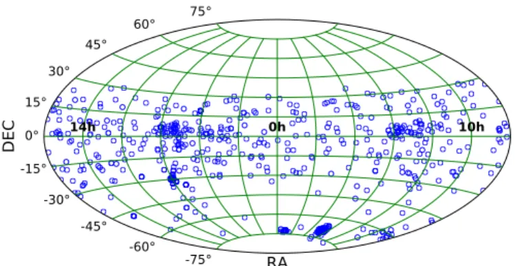
Fig. 1.Positions of XSL stars in the sky (Aitoff projection).

with a wide range of chemical compositions. Our original sam-ple consists of 679 unique stars. The primary references for the construction of the XSL target list were existing spectral libraries or compilations of stellar parameter measurements. In particular, the XSL sample has a strong overlap with the MILES spectral library (142 stars,Sánchez-Blázquez et al. 2006;Cenarro et al. 2007) and the NGSL library (135 stars,Gregg et al. 2006). We completed the list with objects from the parameter compilation PASTEL (Soubiran et al. 2010,2016) and from a variety of more specialised catalogs (see TableA.1for details and corresponding references). In Fig.1we plot the distribution of the selected XSL stars on the sky.

More than half of the stars in the XSL library are red giants in the broad sense, which includes red supergiants or asymptotic giant branch stars. These stars provide strong (age-dependent) contributions to the NIR emission of galaxies (e.g.,Lançon et al. 1999;Maraston 2005;Melbourne et al. 2012). The luminous red stars in XSL are located in star clusters, in the field, in the Galac-tic bulge and in the Magellanic Clouds (TableA.1). A fraction of the asymptotic giant branch stars are carbon stars, whose spectra have been studied in detail byGonneau et al.(2016,2017). We obtained repeated observations for a fraction of the XSL stars (∼20% of our sample), mainly in the cases of luminous cool stars, known or suspected to vary in time.

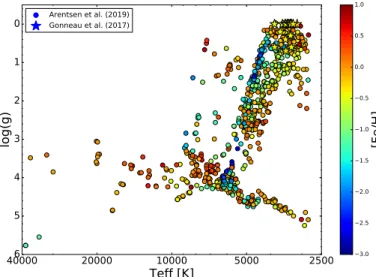
Figure 2 presents the stellar atmospheric parameters cove-rage of the XSL sample as determined byArentsen et al.(2019) andGonneau et al.(2017). We refer the reader to Fig. 2 ofChen et al.(2014) where the HR diagram is presented using literature values. Arentsen et al. (2019) estimated atmospheric parame-ters in a homogeneous manner for 754 XSL spectra of 616 stars: they fit the ultraviolet and visible spectra with the ULySS pack-age (Koleva et al. 2009) using the MILES spectral interpolator (Sharma et al. 2016) as a reference.Gonneau et al.(2017) deter-mined atmospheric parameters of carbon-rich stars by compar-ing the observations to a set of high-resolution synthetic carbon star spectra, based on hydrostatic model atmospheres (Aringer et al. 2016)3_.

The aim of the selection was to obtain representative spectra mapping the widest area of the parameter space defined by the effective temperature (Teff), the surface gravity (log g), and the

iron metallicity ([Fe/H]). Therefore, the sample does not repro-duce the natural frequencies of various stellar types. At the time the target lists were prepared, large public catalogs of homoge-neous stellar parameter estimates were still lacking, and we were unable to populate certain regions of parameters in a satisfactory

3 _{Only the stars less affected by pulsation (namely stars from}

Groups A, B and C as defined inGonneau et al. 2017) are plotted in Fig.2.

2500 5000 10000 20000 40000

Teff [K]

log(g)

[Fe/H]

Fig. 2. Stellar atmospheric parameters, calculated byArentsen et al.

(2019, open symbols) and Gonneau et al. (2017, star symbols), for 769 XSL spectra.

way. In particular, some of the Bulge stars selected on the basis of high estimated metallicities turned out to be less metal-rich than expected (Arentsen et al. 2019).

For applications requiring a higher level of completeness, we note that the X-shooter instrument archive has become a useful source of complementary data over the years. Low mass dwarfs from the archive were combined with XSL data for population synthesis applications by Dries (in prep.). The red supergiants of

Davies et al.(2013) were observed with settings similar to XSL and can usefully complement the XSL library in that region. Finally, the ESO archive4_{contains a very large number of} obser-vations of B-type stars, because these have been used over many years for the correction of telluric absorption. We do not discuss these external data in this article.

2.2. Observing strategy

We gathered the XSL observations in two phases: a pilot pro-gram (periods P84 and P85, October 2009–September 2010) and a Large Program over four semesters (P89-P92, April 2012– March 2014).

We observed each science target with two slit widths. We first took a spectrum with a narrow slit to achieve the required spectral resolution. The narrow-slit widths for the UVB, VIS and NIR arms of X-shooter were 0.500, 0.700, 0.600, respectively, lead-ing to nominal resolutions R= λ/∆λ ∼ 9200, ∼11 000 and ∼7770. With the narrow slits, a wavelength-dependent fraction of the stellar flux is lost. The loss-fraction depends on the seeing, but also on the centering of the star in the slit and on the performance of the atmospheric dispersion corrector of the instrument, both of which are not controlled precisely. The most reliable approach to correct these losses is to observe the targets with a wide slit positioned vertically on the sky. That observation can be cali-brated into absolute flux when conditions are photometric and then can be used to correct the energy distribution of the narrow-slit observation of the same target. In non-photometric condi-tions, as tolerated in our observations (“thin cirrus” tolerance of the ESO VLT scheduling), absolute fluxes cannot be garanteed, but the shape of the energy distribution is properly recovered with this method under the assumption that the cirrus have a flat

4 _{http://archive.eso.org/wdb/wdb/eso/xshooter/form}

transmission curve5. We took wide-slit spectra for every target immediately after the narrow-slit ones, using a 500_{wide slit.}

We performed our observations using the SLIT spectroscopy mode of X-shooter. In this mode three observing strategies are available: STARE, NODDING, and OFFSET. We used each of them depending on the desired outcome. In STARE mode the star was located at the center of the slit and the sky back-ground was estimated from each side of the stellar signal on the observed frame. We used this mode for the wide-slit obser-vations. The NODDING acquisition mode allows observations of the star at two positions (A and B) along the spectrograph slit. In this way we achieved an improved sky subtraction with a double-pass subtraction. Almost all our narrow-slit observations were taken in NODDING mode. An OFFSET acquisition mode alternates between the star and an empty sky region. We used this mode for 12 observations of very bright stars in the pilot program.

2.3. Spectro-photometric standard stars

In order to flux-calibrate our science spectra we used spectro-photometric standard stars (typically white dwarf stars of type DA). These stars were observed once per night using a 500 slit width.

In practice, we used only the five following stars, for which the spectral energy distribution and other parameters are given in the X-shooter manual6_{: BD+17 4708, EG 274, Feige 110,} LTT 3218, and LTT 7987. The other reference stars (CD-32 9927, EG 21, GD 153, GD 71, LTT 1020 and LTT 4364) were discarded either because their spectral energy distribution was not reliably known or because the long exposure times of their default observations (300 or 600 seconds) resulted in saturated NIR K-band spectra.

3. Data reduction and calibration

We have reduced the full set of XSL observations over the pilot and the Large Programs in a uniform manner. This allows us to provide an updated calibration of the spectra initially released under DR1 and to ensure a homogeneity of the present DR2.

Our data reduction and calibration processes are illustrated in Fig.3. We apply the first four steps (referred to as “common data reduction”) to all observations: science target stars and flux standards, wide and narrow slits, and all spectral arms. We use the X-shooter data reduction pipeline (XSH pipeline, Sect.3.1,

Modigliani et al. 2010), up to the creation of two-dimensional (2D) order spectra. Then we extract 1-dimensional (1D) spectra outside of the XSH pipeline to better control the rejection of bad pixels (see Sect.3.2). We further apply corrections for the telluric absorption bands (Sect.3.3) and for the continuous atmospheric extinction (Sect.3.4).

After processing all observations in this uniform way, we derive response curves from the flux-standard spectra (Sect.3.5), and we use these to process both the narrow and wide slit science spectra (Sect. 3.5). Finally, using the wide-slit spec-trum corresponding to each narrow slit observation, we derive a wavelength dependent flux-loss correction and apply it to

5 _{Using the extinction curve for normal cirrus ofLynch & Mazuk} (2001), we find that the ratio of V-band to K-band transmission varies by less than 1% when transmission drops from 100% to 60% because of standard cirrus.

6 _{http://www.eso.org/sci/facilities/paranal/}

Common Data Reduction

Response curve computation

First flux calibration

Flux-loss correction Reduction with the XSH pipeline

One-dimensional extraction

Telluric absorption correction

Atmospheric extinction correction

All observations Flux-standard observations Science observations Science observations

Fig. 3.Overview of the XSL data reduction process.

achieve the final XSL spectrum for each stellar observation (Sect.3.6).

3.1. XSH pipeline

The XSH pipeline consists of a set of data processing mod-ules that perform the individual tasks of the data reduction. These “recipes” can be chained in a flexible way to fulfill the requirement of a specific program. We use the XSH pipeline ver-sion 2.6.8, in physical mode as per the pipeline recommendation. In that mode, the wavelength and spatial scale calibrations are performed by optimising a physical model of the instrument. To achieve a more flexible automation of our process we run the XSH pipeline via the Esorex environment7(version 3.12).

For each science observation, the input to the XSH pipeline is a set of raw data-frames that we identify and collect using the associations of calibration files provided by the ESO archive. When necessary, we modify the default associations to ensure that the flux-standard frames are always reduced with the same flat-field as the corresponding science frames, rather than with the flat-field nearest-in-time (see Sect. 3.5). Saturation was a known problem for several observations of the pilot program but occurred rarely in later semesters. Here, we apply a scheme sim-ilar to that of DR1 to flag strongly saturated observations auto-matically and exclude these from further processing.

We used the default parameters for the creation of the calibration frames (up to the xsh_flexcomp recipe). To trans-form the science and flux-standard frames into flat-fielded,

7 _{https://www.eso.org/sci/software/cpl/esorex.html}

rectified and wavelength-calibrated 2D order spectra, we used recipes xsh_scired_slit_stare for wide-slit observations, and xsh_scired_slit_offset for narrow-slit observations. In particular, we reduced any frames observed in NODDING mode as if they were taken in OFFSET mode, which gives us more flexibility in the handling of bad pixels and improves the quality of our final spectra. In STARE mode, we switch off the sky-subtraction offered by the XSH pipeline because we apply our own algo-rithm during the subsequent 1D-extraction step. Two key para-meters of the above recipes control the sampling of the output spectra along the wavelength axis and along the spatial axis. We set them respectively to 0.015 nm and 0.1600 _{for the UVB and}

VIS arms, and to 0.06 nm and 0.2100for the NIR arm.

The final products of the reduction with the X-shooter pipeline are 2D frames containing the spectral orders of each arm. They include a map of pixel quality flags and a map of the estimated variances of the pixel errors, which we use to propa-gate errors through subsequent processing steps.

3.2. 1D extraction

A main driver for our choice of performing the extraction of 1D spectra outside of the XSH pipeline was the need for more control over the rejection of bad pixels and the sky subtraction. Our extraction procedure follows a prescription adapted from

Horne (1986). It implements a rejection of masked and out-lier pixels, as well as a weighting scheme based on a smooth throughput profile, that can follow residual distortions in the rec-tified 2D-spectra, and on the local pixel-variance as estimated by the earlier steps in the ESO pipeline. The extraction pro-cedure is an updated version of the one presented in Gonneau et al.(2016), and the description below focuses on the modified elements.

3.2.1. Fraction of bad pixels

Before extracting a given order, we double-checked for satura-tion and other invalid pixels by counting the percentage of pixels flaged as bad along the spectrum. The count is restricted to a box extending ±3/±2 pixels (respectively for the UVB/VIS arms and the NIR arm) to either side of the peak of the spatial pro-file of the spectrum. As a general rule, the extraction process is abandoned if more than 30% of the pixels are determined to be bad. Exceptions are implemented for pixels with XSH pipeline-code 6 (unremoved cosmic ray), a warning that we discard to improve the extraction of the observations taken in exception-ally good seeing (see Sect.3.2.5), and for XSH pipeline-code 21 (extrapolated flux in the NIR) in the longest wavelength order of the NIR arm, because keeping those pixels was found to reduce discontinuities between the two last orders of that arm signif-icantly (Gonneau et al. 2016, this is an update with respect to who describe the discontinuities).

3.2.2. Sky background removal

We carried out a sky subtraction for all spectra acquired in STARE mode, as well as for any long-exposure VIS and NIR frames observed in NODDING and OFFSET modes (science frames with exposure times ≥600 s in the VIS and exposure time ≥200 s in the NIR; flux standard frames with exposure time ≥190 s in the VIS and all the NIR frames). The areas along the slit from which the median sky levels are computed are selected in each frame after fitting a Gaussian to the spatial profile of the star, in order to account for the seeing. In STARE mode, these

adjustments avoid artifacts such as the negative fluxes that some-times result from over-subtraction in the standard XSH-pipeline process. In long-exposure spectra, the main purpose is to account for variations in the sky background between the two combined acquisitions.

3.2.3. Updated standard extraction

Horne’s extraction scheme relies on obtaining first a rough guess for the 1D spectrum (that we refer to as the standard spectrum) and then optimizing this extraction with an inverse-variance weighted algorithm, that accounts for the spatial profile of the light at a given wavelength (we call the result the final spectrum). To obtain the standard spectrum, we summed the (sky-subtracted) 2D spectrum along the spatial dimension over a limited range of pixels. We updated our procedure by setting the limits to ±4 or 8 pixels, respectively for NODDING and STARE/OFFSET frames, centered on the peak of the signal. The calculation of the final spectrum is as inGonneau et al.(2016). Along the spatial axis, the ratio of the flux in a pixel to the nor-malized spatial profile is taken as an estimate of the stellar flux at the wavelength of interest and these estimates are averaged with an inverse-variance weight. A limited number of iterations are implemented to add outliers to the bad-pixel mask (maximum 3 at any wavelengths), and these pixels are discarded in the final sum.

3.2.4. Merging of the individual orders

Figure4shows the overlapping orders before merging for each arm of the spectrograph. The flat-fielding algorithm of the XSH pipeline normalizes flat-field frames only globally, hence the blaze function of the instrument is removed in the division by the flat-field, and the extracted orders align well. To merge them, we combined the spectra in the regions of overlap, using weights that combine the inverse variance and a coefficient, α, set to vary linearly from 0 to 1 across those regions. This choice was made because we found that the single-order variance was frequently underestimated at the very end of orders. Hence the flux of each overlapping order, Fmerging, is calculated as follows:

Fmerging=

(1 − α) ∗ FL/VL+ α ∗ FR/VR

((1 − α)/VL+ α/VR)

, (1)

where F and V stand for pixel fluxes and variances, and sub-scripts L and R refer to the spectral orders on the left and right sides of region of overlap.

For the frames observed in NODDING mode, the 1D extrac-tion procedure produces two separate spectra that we averaged together. The end product of this procedure is a continuous 1D spectrum with two extensions: a flux spectrum and an error spectrum.

3.2.5. Chessboard effect

Some of our NIR frames are affected by an issue that we call the “chessboard effect”. When the seeing is exceptional (typically <2 pixels per FWHM of the spectral profile in parts of the raw data), the interpolation scheme used by the XSH pipeline for the geometric transformation into a rectified, wavelength calibrated frame does not perform well. The resulting images (known as ORDER2D frames in the pipeline) display a chessboard pattern as illustrated in the top panel of Fig.5. Because the wavy pat-terns seen along single lines of the rectified 2D-spectrum vary

3500

4000

4500

5000

5500

Wavelength [

]

0

2000

4000

6000

8000

UVB

Extracted, order by order, 1D spectra

6000

7000

8000

9000

10000

Wavelength [

]

0

5000

10000

15000

VIS

12000

16000

20000

24000

Wavelength [

]

0

20000

40000

60000

NIR

Fig. 4. Examples of order-by-order spectra for the three arms (XSL observation X0365). From top to bottom: UVB (12 orders), VIS (15 orders) and NIR (16 orders).

abruptly between one line and the next, the crests of these waves are mistaken for cosmic ray hits.

To deal with this, we first identify pixels with bit code 6 in the quality-mask images produced by the XSH pipeline (flag 6 = unremoved cosmic rays, cf. the bad pixel code conventions in the X-shooter Pipeline Manual) and reset these flags to “good pixel”8. Then, to avoid any re-flagging by our own extraction procedure, we define a “safe zone” in the 2D frame in which any cosmic-ray identification is switched off. This rectangular zone extends to ±4 or 6 pixels on either side of the peak of the spatial profile of the spectrum (respectively for NODDING or for STARE/OFFSET frames). This scheme was also used in a few VIS frames. The bottom panels of Fig.5show an example of a 2D quality-mask before and after editing, and the extent of the safe zone (represented as a blue rectangle). Figure6shows a comparison of the different extraction methods, with and without the flagging and the safe zone, for the ORDER 16 of the NIR arm.

3.3. Telluric absorption correction

We corrected the 1D extracted spectra for telluric absorp-tion with molecfit (Smette et al. 2015;Kausch et al. 2015). Molecfit uses a radiative transfer code and a molecular

8 _{A similar solution is now recommended by ESO on the}

X-shooter FAQ webpage: http://www.eso.org/sci/data-processing/faq/ my-spectrum-of-a-bright-source-looks-much-noisier-than-i-expected-why. html

15800

15900

16000

16100

16200

16300

Spectral dimension [

]

0

5

10

15

20

25

Spatial dimension

INPUT 2D FLUX SPECTRUM (Order 16) for X0648

15800

15900

16000

16100

16200

16300

Spectral dimension [

]

0

5

10

15

20

25

Spatial dimension

INPUT 2D QUALITY MASK

15800

15900

16000

16100

16200

16300

Spectral dimension [

]

0

5

10

15

20

25

Spatial dimension

OPTIMAL 2D MASK

Fig. 5.Example of ORDER2D frame affected by the chessboard effect.

Top:input 2D flux spectrum, before extraction. Middle: input 2D qua-lity mask. Bottom: optimal 2D mask. For both 2D masks, the bad pixels are shown in black and gray.

line database to calculate a synthetic spectrum of the Earth’s atmosphere based on local weather conditions and standard atmospheric profiles. In addition, molecfit also models the instrumental line spread function. Once the characteristics of the instrument have been taken into account, the synthetic transmis-sion spectrum can be used to correct an observed spectrum for telluric absorption.

Table 1 details the relevant parameters that we used for running molecfit. Most of these are taken from Kausch et al. (2015), who also applied molecfit to the processing of X-shooter spectra. In the UVB arm we only corrected for absorp-tion by O3, in the VIS arm we corrected for absorption by H2O,

O2and O3, and in the NIR arm for H2O, CO2, CO, CH4and O2.

Except for water vapor, the abundances of the different mole-cular species are assumed to be constant and equal to the stan-dard atmospheric values. The total amount of water vapor along the pointing direction of the observation is a free parameter of molecfit that can be fit together with the other free parameters. The wavelength regions used for the fitting procedure are speci-fied in Table2. For the NIR arm and the VIS arm, these regions are almost the same as those used inKausch et al.(2015).

It is known that the wavelength calibration of X-shooter is not perfect: Moehler (2015) reports shifts with an aver-age peak-to-peak amplitude of 0.28 pixels, corresponding to 0.0042 nm and 0.0168 nm for our VIS and NIR data, respec-tively. This results in small offsets between the wavelength scale of the spectrum and the synthetic telluric transmission spectrum

15800 16000 16200 16400 16600 16800

Wavelength [Å]

Flux

Standard extraction (black) vs Final extraction [no flagging, no safe zone] (red)

15800 16000 16200 16400 16600 16800

Wavelength [Å]

Flux

Standard extraction (black) vs Final extraction [flagging + safe zone] (red)

Fig. 6. Examples of extracted spectra with the chessboard effect (X0648). The red spectra correspond to the inverse-variance weighted extractions, while the black spectra are for the standard extractions. Upper panel: original extraction, and lower panel: updated extraction to deal with the chessboard effect (flagging and safe zone in the rejec-tion scheme).

Table 1. Parameters of molecfit used to correct XSL spectra for tel-luric absorption. Parameter Value FTOL 0.01 XTOL 0.01 LIST_MOLEC O3 (UVB) H2O O2 O3 (VIS)

H2O CO2 CO CH4 O2 (NIR)

FIT_MOLEC 0 (UVB) 1 0 0 (VIS) 1 0 0 0 0 (NIR) RELCOL 1.0 (UVB) 1.0 1.0 1.0 (VIS) 1.0 1.05 1.0 1.0 1.0 (NIR) FIT_CONT 1 CONT_N 3

CONT_CONST Average of spectrum

FIT_WLC 1 WLC_N 0 WLC_CONST 0.0 FIT_RES_BOX 0 KERNMODE 0 FIT_RES_GAUSS 1 RES_GAUSS 1.0 VARKERN 1

Notes. SeeNoll et al.(2014) for an explanation of the meaning of the different parameters.

produced by molecfit. We alleviate this problem by applying molecfit in a slightly different way. First, we use the “classi-cal” molecfit approach, as described inSmette et al.(2015), to derive the precipitable water vapor column (PWV). Then we cut the spectrum into different wavelength segments. The segments are chosen such that each one contains at least one telluric fea-ture and, if possible, also a “clean” region which is (almost) free of telluric contamination. We fix the PWV parameter to the value found in the first iteration and apply molecfit to each of the wavelength segments. As a final step, the corrected wavelength segments are recombined. Across regions where wavelength

Table 2. Wavelength regions (air) used by molecfit for fitting atmo-spheric transmission spectrum.

Arm Wavelength Molecule region [nm] UVB 302−350 O3 VIS 685−694 O2 VIS 758−777 O2 VIS 929−945 H2O NIR 1120−1130 H2O NIR 1470−1480 H2O NIR 1800−1810 H2O NIR 2060−2070 CO2 NIR 2350−2360 CH4

Notes. For each region, the most important molecule of the transmission spectrum is also given.

segments overlap, we use linearly progressive weights to aver-age the two sets of data.

Our “extended molecfit” approach, where the spectrum of a particular arm is divided into smaller wavelength segments, allows molecfit to find better local wavelength solutions and line spread functions. The final telluric-corrected spectra have a much smaller variance. We use the extended molecfit approach to correct spectra in the VIS and NIR arms. The boundaries of the different wavelength segments are given in Table3. Figure7

compares the two telluric correction approaches: the classi-cal molecfit approach (in gray) and the extended molecfit approach (in red). Figure 8 illustrates the results for the full VIS and NIR wavelength ranges. For the UVB arm, we use the classical molecfit approach since for this arm the wavelength region that contains telluric lines is relatively small.

3.4. Atmospheric extinction correction

Before computing instrument response curves and applying them, the spectra of science and flux-standard stars were cor-rected for observation-specific effects. We corrected the frames for exposure time, gain and continuous atmospheric extinction as follows:

Fout=

Fin

exptime ×gain × 10

(0.4·airmass·extinct)_{, (2)}

where Fin is the flux of the observations as available after

cor-rection for telluric absorption bands. The airmass, exposure time (exptime) and gain were taken from the observation header.

The atmospheric extinction (extinct, expressed in magni-tudes per unit airmass) combines aerosol scattering (Mie diffu-sion, kaero) and Rayleigh scattering (kray), followingPatat et al.

(2011). Molecular absorption (including broad features that are sometimes dealt with like a contribution to the extinction contin-uum) were already accounted for by molecfit. We model the aerosol contribution as advocated byMoehler et al.(2014):

kaero= 0.014 × (λ[µm])−1.38. (3)

The Rayleigh scattering mostly depends on the observation air-mass, and only weakly on the atmospheric conditions. In the zenith direction, we model it as:

kray= p 1013.25× (0.00864+6.5×10 −6 H) × λ−(3.916+0.074λ+0.050/λ), (4)

Table 3. Wavelength segments (air) used for the extended molecfit approach, as described in the text.

Arm Wavelength Arm Wavelength segment [nm] segment [nm]

VIS λstart−637 NIR λstart−1105

VIS 633−712 NIR 1095−1185

VIS 708−752 NIR 1175−1255

VIS 748−782 NIR 1245−1305

VIS 778−862 NIR 1295−1455

VIS 858−926 NIR 1445−1605

VIS 922−λend NIR 1595−1755

NIR 1745−1880 NIR 1870−1985 NIR 1975−2040 NIR 2030−2085 NIR 2075−2285 NIR 2275−2385 NIR 2375−λend

Notes. The extended molecfit approach is only used for the VIS arm and the NIR arm.

with pressure p= 744 hPa, height H = 2.64 km and wavelength λ in µm (values fromNoll et al. 2012).

Figure9compares our extinction curve to the XSH pipeline one. From the bottom panel of that figure, we can see that the main differences are in the ozone Huggins bands, which are not deep enough in the reference curve.

3.5. Response curve and first flux calibration

In the XSH pipeline the 2D flat-field spectra are not norma-lized across the surface of each grating order before they are divided into the program data. Hence the division corrects both the pixel-to-pixel variations of the sensitivity of the detector and major transmissions variations, such as those produced by the blaze functions of the gratings. This choice ensures that extracted single-order spectra within one arm are easily con-nectable. In exchange for this benefit, the arm-spectra (as illus-trated in Figs. 4 and 8) contain an imprint of the (inverted) spectra of the lamps used to illuminate the flat-field exposures. Unfortunately, the X-shooter flat-field lamps are less stable than other elements of the acquisition chain, in particular in the NIR arm. Hence, when pairing observations of a science target and of a spectro-photometric standard star, it is recommended to use the same flat-field images for the two data sets9_.

To determine a response curve from the 1D spectrum of a flux standard, we performed a χ2_{-minimization between that}

observation on one hand, and the product of its theoretical spec-trum and the unknown response curve on the other. The response curve is represented with a high-order spline polynomial. The typical number of spline nodes is 35 for the UVB and NIR arms and 60 for the VIS. These spline nodes are not all regu-larly spaced; they are placed sparsely where spurious oscilla-tions should be avoided (e.g., across the telluric water bands in the NIR arm) and more tightly where small-scale instru-mental effects must be accounted for (e.g., features at 365 nm due to the combination of two different flat-fields in the UVB

9 _{Seehttp://www.eso.org/observing/dfo/quality/XSHOOTER}

/qc/problems/problems_xshooter.html#NIR_FF; current recom-mendations extend to the VIS and UVB arms.

685 695

no

rm

al

iz

ed

flu

x

[a

rb

it

ra

ry

un

it

s]

λ

[nm]

no

rm

al

iz

ed

flu

x

[a

rb

it

ra

ry

un

it

s]

λ

[nm]

Fig. 7. Comparison between telluric correction with the classical molecfit approach (MF TC) and with the extended molecfit approach (extended MF TC). The upper star corresponds to a flux-standard star and the lower star to X0073 (HD 18769). The figure shows different telluric regions in the VIS arm and NIR arm. Within each of these regions, the corrected spectrum is normalized to unit mean.

arm10, the dichroic features at 560-620 nm11, a flat-field bump at 2100 nm; seeMoehler et al. 2014for more details). Furthermore, we masked the Balmer lines in the UVB and VIS arms, the O2

lines in the VIS and the deepest telluric regions in the NIR. We used the response curves for a first flux-calibration of the science spectra both for the narrow and wide slit obser-vations. The resulting intensities are physical flux densities, in erg s−1_cm−2_Å−1_{. These spectra are cleaned from the}

atmo-spheric and instrumental effects, except for the slit losses. The narrow-slit spectra, in particular, still do not reflect the absolute distribution of the stellar flux.

3.6. Flux-loss correction and final energy distributions For 85% of the spectra, wide-slit observations of sufficient qua-lity are available, and thus the narrow-slit spectra are corrected for wavelength-dependent flux-losses. To this end, we computed a smoothed version of the ratio of the wide-slit over the narrow-slit spectrum, and then fit a low-order polynomial (typically of order 1 for UVB/VIS frames, and 3 for NIR frames). Finally, we multiplied our narrow-slit spectra by this polynomial. In a few cases (3 observations of 2 a priori non-variable stars, namely X0194 [HD 193281] and X0306/X0311 [HD 29391]), when only one of several observations of the same star had an associ-ated wide-slit spectrum or an otherwise more reliable continuum,

10 _{https://www.eso.org/observing/dfo/quality/XSHOOTER/} pipeline/pipe_problems.html#uvb_flux 11 _{https://www.eso.org/sci/facilities/paranal/} instruments/xshooter/knownpb.html

6000

7000

8000

9000

10000

Wavelength [

]

0

5000

10000

15000

VIS

12000

16000

20000

24000

Wavelength [

]

0

20000

40000

60000

NIR

Fig. 8.Before (black) and after (red) the telluric absorption correction process for X0365 (VIS and NIR arms).

that observation was used as a reference for the other observa-tion(s).

In summary, our data reduction procedure uses the ESO pipeline until the 2D spectra are rectified and wavelength-calibrated. Subsequent steps were adjusted, mainly to improve the usage of pixel-flags, the sky subtraction, the telluric correction

3500 4000 4500 5000 5500 Wavelength [Å] 0 40000 80000 120000 UVB

Before (black) / After (red) the telluric absorption correction step

3000 3500 4000 4500 5000 5500 Wavelength [Å] 0.0 0.2 0.4 0.6 0.8 1.0 Transmission Transmission = 10^(-0.4*airmass*atmospheric_extinction)

Ozone (from Molecfit) Aerosol Rayleigh scattering

Our transmission curve * Ozone (from Molecfit) Paranal transmission curve

3000 3500 4000 4500 5000 5500 Wavelength [Å] 0.80 0.85 0.90 0.95 1.00 1.05 1.10

Ratios of the transmissions

Paranal-based transmission / our transmission

Fig. 9.Top:UVB flux-standard spectrum (related to X0365) corrected for O3 with Molecfit (red spectrum), compared to an uncorrected one (black spectrum). Middle: our own transmission curve (red curve) – with the details of its three components – compared to the pipeline one (black curve). Bottom: ratios of the transmissions.

and the combined usage of narrow-slit and broad-slit observation for flux calibration. 85% of the DR2 spectra are flux calibrated in the sense that they are corrected for all stable transmission factors of the acquisition chain, and for wavelength-dependent losses due to the narrow widths of the slits that provide the desired spectral resolution. Residual flux calibration errors may come from changes in telescope+instrument+sky transmission-curves between the observations of the science targets and of the spec-trophotometric standard star, and from residual slit losses in the broad-slit observations. They are assessed via comparisons with external data sets in Sect.4.5. A few examples of final DR2 spec-tra can be found in Fig.10.

4. Properties of the DR2 spectra

In this section we present an assessment of the overall prop-erties of the spectra, including the quality of the wavelength and flux calibration, and properties of the line-spread function. We describe the quality flags associated with each published spectrum.

4.1. Typical signal-to-noise ratios

Figure11 shows the distribution of the median signal-to-noise ratios (S/Ns) per pixel for our observations. Except for the coolest stars, typical S/N values are about 70, 90 and 96 for the

UVB, VIS and NIR arms respectively. In fact, the S/N for cool stars (Teff < 5000 K) varies drastically with wavelength across

the UVB arm. S/N similar to those of warmer stars are found in a temperature-dependent range of wavelength toward the red end of that arm.

Correlations between the errors in neighboring pixels are expected as a result of the redistribution of pixel fluxes when the original 2D-images are transformed into rectified order-images. They depend on the observation mode, on the seeing and on wavelength in a complex fashion. We have not attempted to cha-racterize them in detail. In general however, they would extend over a few pixels, on a wavelength range similar to the (arm-dependent) resolution element of the spectra.

4.2. Spectral resolution and line spread function

We have determined the spectral resolution and the line spread function for each arm with the Penalized PiXel-Fitting method (pPXF,Cappellari & Emsellem 2004;Cappellari 2017), using a subset of the PHOENIX theoretical spectral library (Husser et al. 2013) as templates. The available PHOENIX library samples effective temperatures with a step of 200 K (or of 500 K above 12 000 K), surface gravities with a step of 0.5 dex, and [Fe/H] with a step of 0.5 dex (or of 1 dex where [Fe/H] < −1). The sub-set retained contains the 388 theoretical stars that are closest to the XSL library stars in the stellar parameter space, based on the stellar parameters derived from XSL observations byArentsen et al.(2019).

All XSL UVB, VIS and NIR spectra were fit one 200 Å-wide wavelength region at a time. In the NIR, the telluric-contaminated regions (13 500–14 200 Å and 17 700–21 000 Å) were not analyzed.

4.2.1. The spectral resolution

The spectral resolution is described by the velocity dispersion measurements of the pPXF fit, as the template spectrum has a much higher resolution (R ∼ 500 000,Husser et al. 2013) than the X-shooter spectra (R ∼ 10 000). As the observations span multiple observing periods, the measurements for stars from dif-ferent observing periods were analyzed separately and then com-bined. In each observing period, the velocity dispersion results from the pPXF fitting were sigma-clipped with a 5-σ threshold. Sigma-clipping was iterated until convergence was achieved.

Figure12shows the wavelength dependence of the resolu-tion for each observing period and X-shooter arm. The 1 σ error bars belong to period P90 measurements, but are similar for all observing periods. The scatter around the median value comes from stars with lower S/N or a low number of spectral lines in each wavelength region. The red points show the weighted averages of the medians of all observing periods. The resolu-tion is stable throughout the observing periods, with only P84 observations showing slightly lower resolution. The resolution R= λ/∆λ is also relatively constant with wavelength, although

Chen et al.(2014) initially showed otherwise for the UVB arm. However, they only used the F, G, K stars of observing periods P84 and P85. The adopted spectral resolution for each arm is the average value over all wavelengths: 13 ± 1 km s−1_{for UVB,}

11 ± 1 km s−1for VIS, and 16 ± 1 km s−1for NIR. These values are shown with the black dashed lines and the ±1σ gray shaded areas in Fig.12.

The spectral resolution measures are converted from σ to FWHM assuming Gaussian line profiles in velocity space (FWHM= 2.35σ) and used to re-evaluate the resolving power

4000

8000

12000

20000

Wavelength [

Å

]

0

10

20

30

40

50

Relative flux

HD 57060 (X0116, O7)

HD 147550 (X0245, B9V)

HD 175058 (X0646, A5IV)

HD 110885 (X0900, F3V)

BD-01 1792 (X0843, G6V)

HD 119802 (X0379, K3V)

HIP 75423 (X0683, M2V)

Y Sge (X0761, M4)

ISO-MCMS J005712.2-730704 (X0013, C)

Fig. 10.Typical XSL spectra in the OBAFGKMC sequence in log-scale of wavelength. For each star, the corresponding XSL observation number and spectral type are indicated in brackets. The gaps indicate the overlap regions between consecutive arms. Gray bands mask the deepest telluric regions in the NIR arm, as well as a few other local artifacts.

R= c/FWHM (c being the speed of light). Our adopted values are close to the nominal ones12_{, as can be seen in Table4.}

12 _{https://www.eso.org/sci/facilities/paranal/}

instruments/xshooter/inst.html

4.2.2. The shape of the line spread function

The deviations of the line spread function (LSF) from a Gaus-sian are described with Gauss-Hermite velocity moments h3

and h4, which are related to skewness and kurtosis respectively.

0 100 200 300 400 500 0.000 0.005 0.010 0.015 0.020 0.025

Density

Median S/N (Hot stars): 73.99 Median S/N (Cool stars): 17.09

Distribution of signal-to-noise ratios

UVB arm Hot stars Cool stars (< 5000 K) 0 100 200 300 400 500 0.000 0.002 0.004 0.006 0.008 0.010 0.012

Density

Median S/N (Hot stars): 91.44 Median S/N (Cool stars): 62.68

VIS arm Hot stars Cool stars (< 5000 K)

0 100 200 300 400 500

Median S/N per spectrum

0.000 0.001 0.002 0.003 0.004 0.005 0.006 0.007 0.008

Density

Median S/N (Hot stars): 96.77 Median S/N (Cool stars): 96.01

NIR arm Hot stars Cool stars (< 5000 K)

Fig. 11.Distribution of the signal-to-noise ratio per arm.

signal-to-noise ratio is excellent. Therefore, h3and h4

measure-ments from all observing periods were analyzed together. We computed the S/N in each wavelength bin (window of 200 Å each) and rejected measurements from spectra with S /N < 200. Additionally, measurements from the very blue wavelengths, λ < 3600 Å, were not included due to low signal. The Gauss-Hermite moments were finally computed from 6510 highest-quality pPXF measurements. Table 5 shows the median and the standard deviation of the results per arm. To within one standard deviation, the line spread function in all arms is a Gaussian.

4.3. Rest-frame velocity correction

The DR2 data are corrected for radial velocity and provided in the rest-frame (with wavelengths in air). The barycentric radial velocities, cz, were estimated separately in each of the three arms, because differences between arms are common and often in excess of 10 km s−1 (see Moehler 2015, for a discussion). The cz values are available in the header of the final FITS files, together with the barycentric corrections we applied13.

In the UVB and VIS arms, the final estimates were obtained with the ULySS package (Koleva et al. 2009) and the ELODIE 3.2 spectral interpolator (Wu et al. 2011), as also used in the study of stellar parameters ofArentsen et al.(2019). This full-spectrum fitting approach requires an approximate a priori knowledge of the radial velocity for the method to converge, because it performs a local minimization using a Levenberg-Marquardt algorithm. The accuracy of the cz guess should be better than a few times the FWHM of the spectral lines. At the

13 _{The barycentric radial velocity is the sum of the topocentric velocity} and the barycentric correction.

resolution of XSL, the FWHM of the lines is on the order of 30 km s−1_{, and since the barycentric velocities of the Galactic}

and LMC/SMC XSL stars are expected to span a range of up to about 400 km s−1, we repeated the fit starting with a series of cz guess in the interval from −300 to +300 km s−1 _{with a step of}

100 km s−1. For each value of the guess, the atmospheric param-eters Teff, log g and [Fe/H] as well as cz and the broadening were

re-adjusted. The solution with the lowest χ2was adopted. In the NIR, the adopted values of cz were estimated by cross-correlation with the nearest model in the library of syn-thetic spectra ofHusser et al.(2013). Starting from the estimated parameters ofArentsen et al.(2019), we used χ2_{-minimization to}

identify an adequate NIR representation of each NIR spectrum. The spectral ranges used for the cross-correlation were adjusted based on the effective temperature and spectral type, in order to include a sufficient number of spectral features. In the coolest stars, we avoided regions dominated by a single steep molecular bandhead, as the resulting cz then depend on the way the spec-tra are renormalized to remove the dominant slope, before the cross-correlation.

For some spectra of cool stars, it was not possible to deter-mine cz in the UVB, or even in the VIS, because of an insu ffi-cient flux. When a measurement in the NIR was available, we then simply assigned the latter to the UVB and VIS.

During the preparation of DR2, several methods other than those finally adopted were employed to re-estimate the radial velocities of various data subsets. The distributions of velocity differences between methods typically display an approximately Gaussian peak, with a standard deviation of 2 to 3 km s−1; non-Gaussian tails of the distributions typically contain ∼13%, ∼18% and ∼10% of the stars in the UVB, the VIS and the NIR arms. Hence the value of 2 to 3 km s−1_{is representative of the}

uncer-tainties on the rest-frame wavelengths of the DR2 data. 4.4. Quality assurance

After the data reduction, we assigned a number of quality flags to our data based on visual inspection and on experience gained by comparing the observations with synthetic or other empirical spectra (e.g.,Gonneau et al. 2017;Lançon et al. 2018;Arentsen et al. 2019). Table8(item “Quality flags (per arm)”) describes our flags. The flags were added to the headers of the final FITS files, and peculiarities specific to individual spectra are listed in TableB.1. We note that this list is not exhaustive, as some arti-facts might have been overlooked.

More generic caveats concerning the data are the follow-ing. In the UVB, the spectra tend to be wavy near 0.35 µm (the combination of two different flat-fields D2 and QTH in this range leads to errors, see footnote10_{) and between 0.545–0.55 µm} (known instabilities of the transmission of the dichroic plate that feeds the UVB and VIS arms of X-shooter, see footnote11).

For the VIS arm, frequent artifacts are seen in the spectral shape between 0.54–0.59 µm (dichroic issue, see footnote11). The continuum at the red end, beyond 0.97 µm, can also have some artifacts (second dichroic region; effect >5%). Molec-fit corrects only for molecular absorption lines, hence telluric absorption by metals is not removed (an example is the frequent contamination of the stellar NaI doublet by telluric Na, between 588 and 592 nm).

In the NIR, a step sometimes arises between the two reddest orders (near 2.25 µm). The noise spectrum does not capture the 1.1 µm telluric band sufficiently strongly. The slope of the spec-trum is sometimes poorly determined below 1.05 µm (dichroic region; effect >5%). The K-band is usually of poor quality for

3500

4000

4500

5000

5500

10

15

20

UVB

UVB

= 13 ± 1 km s

1

6000

6500

7000

7500

8000

8500

9000

9500

10000

10

15

20

(k

m

s

1

)

_VIS

_VIS

_{= 11 ± 1 km s}

1

10000

12000

14000

16000

18000

20000

22000

24000

wavelength (Å)

10

15

20

25

NIR

NIR

= 16 ± 1 km s

1

P84

P85

P89

P90

P91

P92

Fig. 12.Spectral resolution wavelength dependence for each observing periods. Gray, black, green, blue, dark blue and indigo markers show the medians of measurements of data from observing periods “P84”, “P85”, “P89”, “P90”, “P91” and “P92” respectively. The red point shows the weighted average of all observing periods. The error bars belong to period P90 measurements and are shown for illustrative purposes.

Table 4. Adopted spectral resolution values per arm.

Arm σ FW H M R R

[km s−1] [km s−1] (our values) (nominal values)

UVB 13 30.61 9793 9700

VIS 11 25.90 11 573 11 400

NIR 16 37.68 7956 8100

hot stars (K-band contiuum wavy, lower S/N). Some of these stars are flagged with HAIR_NIR (meaning that there are some narrow spikes in the NIR spectrum, cf Table8).

4.5. Photometric comparison

Chen et al.(2014) compared the DR1 (UVB and VIS) spectra with literature spectra taken from NGSL (Gregg et al. 2006), the calcium-triplet library CaT (Cenarro et al. 2001), and also with higher-resolution spectral libraries such as UVES POP (Bagnulo et al. 2003) and ELODIE (Prugniel & Soubiran 2001). They found a good agreement in the line shapes and depths between XSL and these libraries.

Here we focus on the broad-band spectral energy distribu-tion across the single-arm spectra of DR2. Based on synthetic photometry, we compare colors within the UVB and VIS arms to those of the MILES library (Sánchez-Blázquez et al. 2006); in the NIR, we confront the XSL colors with those of the 2MASS survey (Cohen et al. 2003;Skrutskie et al. 2006), and with syn-thetic colors of the IRTF/E-IRTF spectra (Rayner et al. 2009;

Villaume et al. 2017).

Table 5. Line-spread function parameters h3and h4.

UVB VIS NIR

h3 0.00 (0.06) −0.03 (0.06) 0.03 (0.05)

h4 −0.03 (0.09) −0.01 (0.07) −0.01 (0.06)

Table 6. Artificial filters used in Sect.4.5.1.

Reference set Filter λmin[Å] λmax[Å]

MILES box1 3900 4500

box2 4600 5200

box3 5400 6200

box4 6300 7100

4.5.1. Comparison with MILES

Many of the XSL stars were initially selected from the MILES collection (Sánchez-Blázquez et al. 2006). Forty MILES stars were present in XSL DR1, andChen et al.(2014) found a good agreement between these data in the UVB and VIS arms. In the present release, 173 spectra of 142 stars have a MILES counter-part, of which 164 are corrected for slit-losses. To avoid com-plications due to the edges of the X-shooter arms, we define artificial broad-band filters to compare the synthetic photometry of the two data sets (Table6and Fig.13).

Figure 14 shows how the MILES and XSL synthetic col-ors compare. We find excellent agreement in general, with a mean offset of −0.005/−0.01 mag and an rms scatter of

Fig. 13.Filters designed for the comparison with MILES spectra, over-laid on the XSL spectrum of a cool star. The filters avoid the spec-tral regions most strongly affected by the unstable dichroic between the UVB and VIS arms (plotted in gray).

0.056/0.032 mag, respectively for colors (box1−box2) and (box3−box4). We have examined outliers with color differences larger than 0.1 mag individually, using plots of the spectra and the extensive comparison of XSL spectra with the theoretical spectra ofHusser et al.(2013) that is the subject of another arti-cle (in prep.). The arti-clear outlier at the red extreme in the bot-tom panel is BD+19 5116B (XSL observation X0440, spectral type M4.0Ve), a flare star. We observed this star at a different phase than MILES. The star is also an outlier in (box1−box2). Six other outliers at the red end of (box1−box2) are cluster stars. Five of these are in NGC 6838. We trust their XSL energy dis-tributions to better than 10% because the comparison of these spectra with reddened theoretical models raises no alarms and leads to an extinction estimate that agrees with the values listed inDi Cecco et al.(2015) for the cluster (article in preparation). One object is in NGC 1904, and again best-fit models are not alarming and agree with the very small reddening toward that cluster found in the literature. Still in (box1−box2), the bluest outlier is a hot star, which is also represented very well with models. Removing those outliers, the rms scatter in (box1−box2) drops from 0.056 to 0.030 mag. The two outliers in (box3−box4) not yet discussed are the hot star just mentioned, and an F-type star for which the fit with model spectra excludes large error on the slope in the VIS arm. Removing these, the rms scatter for (box3−box4) drops from 0.032 to 0.022 mag. Table7 summa-rizes these dispersion measurements.

4.5.2. Comparison with 2MASS

The 2MASS filters J, H and Ksfit entirely into the wavelength

range of the NIR arm of X-shooter, as seen in Fig.15. We com-pute synthetic photometry compatible with 2MASS using the relative spectral response curves and reference fluxes ofCohen et al. (2003). The 2MASS filters J, H and Ks fit entirely into

the wavelength range of the NIR arm of X-shooter, as seen in Fig.15).

Figure16shows the results of the comparison. Overall there is good agreement. Small systematic offsets indicate small zero point errors in the exercise; they are in opposite directions for (J − H) and (H − Ks), suggesting a normalization difference

in the H band (as also mentioned inVillaume et al. 2017). We find an rms scatter around the mean of 0.050 mag for (J − H) and 0.053 mag for (H − Ks). After removing the contribution

explained by 2MASS errors in quadrature, the residual scatter

Fig. 14. Comparison of synthetic colors between XSL and MILES. Only XSL-spectra with slit-loss corrections are used.

Table 7. Standard deviations of the color-differences between XSL and external data sets.

External Color Std. dev. Comments

reference σ [mag]

MILES (box1−box2) 0.030 0.056 incl. 7 outliers MILES (box3−box4) 0.022 0.032 incl. 3 outliers 2MASS (J − H) 0.032 0.050 incl. 2MASS errors 2MASS (H − Ks) 0.038 0.056 incl. 2MASS errors

IRTF (J − H) 0.023 0.033 incl. 6 outliers IRTF (H − Ks) 0.019 0.029 incl. 4 outliers Notes. The outliers are not the same for all colors. The 2MASS standard deviations listed each include six 4-σ outliers. See text for details.

is of 0.032 mag in (J − H) and 0.038 mag in (H − Ks). These are

still conservative estimates of the errors in the NIR XSL colors, which are clarified in Sect.4.5.3. In both panels, the larger dis-persion toward redder objects is due to cool stars (M and C stars,

Fig. 15.Response curves of the 2MASS filters, overlaid on an XSL spectrum. The transmission curves are taken fromCohen et al.(2003).

and stars with Te_ff < 3500 K), of which many are known or

sus-pected variables.

4.5.3. Comparison with IRTF

Empirical NIR spectral libraries are still rare in the literature. We choose to compare XSL with the IRTF spectral library (Rayner et al. 2009) and its later extension (hereafter E-IRTF,Villaume et al. 2017) as their wavelength range overlaps with ours (0.7– 2.5 µm) and the spectra are flux-calibrated. Their resolution is R ∼ 2000, and their S/Ns are on the order of 100. IRTF con-tains mainly solar-metallicity stars with spectral types between F and M, plus some AGB stars and L dwarfs. E-IRTF extends the metallicity coverage of IRTF for late-type stars from mainly solar to −1.7 < [Fe/H] < 0.3. Our sample counts 19 stars in common with IRTF (in practice 25 XSL spectra) and 48 stars in common with E-IRTF (61 XSL spectra), The cross-match between XSL and IRTF then corresponds to 86 spectra in total, and 77 when we restrict the sample to XSL spectra with slit-loss corrections.

Figure17shows the comparison. We find a good agreement with insignificant offsets (6 0.007 mag) and an initial rms scatter of 0.033 and 0.029 mag, respectively for (J −H) and (H−Ks). We

checked all the outliers individually (respectively 6 and 4 cases for these two colors), by overplotting the IRTF and XSL spec-tra on one hand, and by inspecting the comparison of the XSL spectra with best-fit stellar models on the other. One outlier is a Mira that indeed varied in spectral type between the observa-tions. Another is a star listed as abnormal in TableB.1(X0878). For all other cases, the IRTF SEDs show signs of a discontinuity between the J and the H band, while the comparison between the XSL and the theoretical spectra essentially excludes errors larger than a few percent. Removing the 6 suspicious cases from the sample, the scatter drops to 0.023 mag in (J − H) and 0.019 mag in (H − Ks). Hence a representative value of our internal

uncer-tainties in these NIR colors, at least for this subsample, is 2%.

5. Final data products and availability

The final data products released as DR2 consist of single-arms spectra, with linearly sampled wavelengths in the rest-frame. The spectra are provided as FITS binary tables, each contain-ing three columns: the wavelength (in nm), the flux spectrum (in erg s−1cm−2Å−1), and an error spectrum (in the same units). A set of keywords in the headers of the FITS files keep track

Fig. 16. Comparison of synthetic colors between XSL and 2MASS. Only XSL-spectra with slit-loss corrections are used. The brown points correspond to cool stars (Teff < 3500 K or spectral type M and C). The legends provide the average offset between the colors of the two data sets, the rms scatter around the mean, as well as the part of the rms scatter that is explained by the 2MASS error bars shown in the bottom panels.

of various steps of the data-reduction and calibration processes, and of results of the quality assessments. A (non-exhaustive) list of these keywords is given in Table8.

The DR2 spectra are made available as two separate sets. The first contains those spectra for which a correction for flux-losses across the spectrograph slit was possible, as described in Sect.3.6). It represents 85% of the observations. We choose to also deliver the remaining 15% of the spectra, for which the flux-losses could not be estimated and corrected. They are identified via header keyword LOSS_COR, which is then set to F. The data can be downloaded from the XSL website, from the CDS interface or from the ESO Phase 3 interface.

6. Concluding remarks

In Chen et al.(2014), we release 246 near-ultraviolet and vis-ible spectra for 237 stars. In this paper, we present the second data release of the X-shooter Spectral Library, which consists of

Fig. 17.Comparison of synthetic colors between XSL and IRTF (open circles for IRTF and filled circles for E-IRTF). The brown symbols cor-respond to cool stars (M/C stars, and stars with no spectral type and Teff < 3500 K).

all the spectra observed as part of this Large Program, in all the three wavelength ranges of the instrument. The major addition of this release is the NIR data, which extends out to 2.5 µm. The simultaneous optical and NIR observations in this unique data set eliminate a major risk of inconsistencies that has prevailed in previous empirical multi-wavelength libraries based on indepen-dent samples in the two wavelength regions. The library contains 2388 spectra of 666 unique stars, at a resolution R ∼ 10 000. This corresponds to 791 UVB spectra, 811 VIS spectra and 786 NIR spectra of these stars.

All the spectra, including those previously released, have been reduced in a homogeneous way with updated algorithms. They were corrected for atmospheric extinction and telluric absorption, which maximizes the wavelength ranges suitable for scientific exploitation. In particular, the wings of the water bands of the atmospheres of cool stars in the NIR arm can be measured, and synthetic photometry can be exploited across wavelength regions where it would otherwise be close to meaningless.

The observational setup and the data reduction were tailored to achieve a good relative flux calibration of the spectra, prior-itizing the energy distributions over absolute fluxes. This effort was driven by two main scientific applications foreseen for XSL. In population synthesis calculations, the energy distributions are important in determining the relative fluxes of various stars at different wavelengths. They are also relevant if the data are used to test how well current theoretical stellar models are able to reproduce observed colors and spectral features simultaneously. Flux calibration is notoriously difficult to achieve with slit-fed echelle spectrographs and X-shooter is no exception. 85% of the DR2 spectra are flux calibrated in the sense that they are cor-rected for all stable transmission factors of the acquisition chain, and for wavelength-dependent losses due to the narrow widths of the slits that ensured the desired spectral resolution. For these 85%, residual flux calibration errors may come from changes in telescope+instrument+sky transmission curves between the observations of the science targets and of the spectrophoto-metric standard star, and from residual slit losses in broad-slit observations. The remaining 15% of the DR2 spectra are not corrected for slit-losss, because the matching broad-slit obser-vations were faulty. Systematic differences of the energy distri-butions with those of previous libraries, if any, are small: the average differences between the synthetic colors measured on XSL spectra (after slit-loss correction) and on spectra from Miles or (E-)IRTF are below 1%; the dispersion in these comparisons indicates typical individual errors on these broad-band colors, outside the main telluric regions, of 2 to 4% in XSL (with some outliers). Anticipating future publications, we note that compar-isons with theoretical spectral libraries across the HR-diagram show clear systematic differences that depend on location in that diagram, with excellent matches in some regions and o ff-sets in certain colors in others; this demonstrates that the current flux calibration allows us to address the scientific questions that were planned. We note that it may be possible to improve the spectrophotometry of XSL spectra in the future, at least at opti-cal wavelengths, pending on additional observations with other instruments (e.g., the integral-field spectrograph MUSE, as sug-gested byIvanov et al. 2019).

The residual errors in the relative flux scales of the spec-tra of the three arms of X-shooter are generally smaller than a few percent. However, there are exceptions, and merging the arms for all the DR2 spectra is a non-trivial process. As previ-ously mentioned, simply fitting the observations to (adequately reddened) theoretical spectra does not provide immediately use-ful re-scaling factors, as available collections of models do not match the observed energy distributions sufficiently well in all parts of the HR diagram (again, the systematics in these trends show that the issues are not artifacts of flux calibration proce-dures). Work on merging the arm-spectra is ongoing (Verro, in prep.). This work is tied to the development of a spectral inter-polator for XSL, which is needed to predict XSL-based spectra along the isochrones of artificial stellar populations. The com-parison between interpolated and original library spectra helps identifying and correcting merged spectra for which the initial relative scaling is inadequate.

The DR2 spectra are made available in the restframe, with radial velocity information in the headers. While the restframe calibration is accurate to typically better than 2 km s−1_{, the radial}

velocity estimates are affected by larger instrumental instabilities and should be regarded with caution.

Because XSL extends into the NIR, it emphasises cool and infrared-luminous stars which otherwise tend to be scarce in stellar libraries. Studying the AGB stars and red supergiants by