SAGE III aerosol extinction validation in the Arctic winter: comparisons with SAGE II and POAM III

(1)

HAL Id: hal-00302271

https://hal.archives-ouvertes.fr/hal-00302271

Submitted on 16 Nov 2006

HAL is a multi-disciplinary open access

archive for the deposit and dissemination of sci-entific research documents, whether they are pub-lished or not. The documents may come from teaching and research institutions in France or abroad, or from public or private research centers.

L’archive ouverte pluridisciplinaire HAL, est destinée au dépôt et à la diffusion de documents scientifiques de niveau recherche, publiés ou non, émanant des établissements d’enseignement et de recherche français ou étrangers, des laboratoires publics ou privés.

SAGE III aerosol extinction validation in the Arctic

winter: comparisons with SAGE II and POAM III

L. W. Thomason, L. R. Poole, C. E. Randall

To cite this version:

L. W. Thomason, L. R. Poole, C. E. Randall. SAGE III aerosol extinction validation in the Arctic winter: comparisons with SAGE II and POAM III. Atmospheric Chemistry and Physics Discussions, European Geosciences Union, 2006, 6 (6), pp.11357-11389. �hal-00302271�

(2)

ACPD

6, 11357–11389, 2006

SAGE III aerosol extinction validation L. W. Thomason et al. Title Page Abstract Introduction Conclusions References Tables Figures ◭ ◮ ◭ ◮ Back Close

Full Screen / Esc

Printer-friendly Version Interactive Discussion

EGU Atmos. Chem. Phys. Discuss., 6, 11357–11389, 2006

www.atmos-chem-phys-discuss.net/6/11357/2006/ © Author(s) 2006. This work is licensed

under a Creative Commons License.

Atmospheric Chemistry and Physics Discussions

SAGE III aerosol extinction validation in

the Arctic winter: comparisons with SAGE

II and POAM III

L. W. Thomason1, L. R. Poole1, and C. E. Randall3

1

NASA Langley Research Center, Hampton, Virginia, USA

2

Science Applications International Corporation, Hampton, Virginia, USA

3

University of Colorado, Boulder, Colorado, USA

Received: 21 September 2006 – Accepted: 8 November 2006 – Published: 16 November 2006

(3)

ACPD

6, 11357–11389, 2006

Full Screen / Esc

EGU

Abstract

The use of SAGE III multiwavelength aerosol extinction coefficient measurements to infer PSC type is contingent on the robustness of both the extinction magnitude and its spectral variation. Past validation with SAGE II and other similar measurements has shown that the SAGE III extinction coefficient measurements are reliable though the 5

comparisons have been greatly weighted toward measurements made at mid-latitudes. Some aerosol comparisons made in the Arctic winter as a part of SOLVE II suggested that SAGE III values, particularly at longer wavelengths, are too small with the implica-tion that both the magnitude and the wavelength dependence are not reliable. Com-parisons with POAM III have also suggested a similar discrepancy. Herein, we use 10

SAGE II data as a common standard for comparison of SAGE III and POAM III mea-surements in the Arctic winters of 2002/2003 through 2004/2005. During the winter, SAGE II measurements are made infrequently at the same latitudes as these instru-ments. We have mitigated this problem through the use potential vorticity as a spatial coordinate and thus greatly increased the number of coincident events. We find that 15

SAGE II and III extinction coefficient measurements show a high degree of compatibility at both 1020 nm and 450 nm except a 10–20% bias at both wavelengths. In addition, the 452 to 1020 nm extinction ratio shows a consistent bias of ∼30% throughout the lower stratosphere. We also find that SAGE II and POAM III are on average consistent though the comparisons show a much higher variability and larger bias than SAGE II/III 20

comparisons. In addition, we find that the two data sets are not well correlated below 18 km. Overall, we find both the extinction values and the spectral dependence from SAGE III are robust and we find no evidence of a significant defect within the Arctic vortex.

(4)

ACPD

6, 11357–11389, 2006

Full Screen / Esc

EGU

1 Introduction

The Stratospheric Aerosol and Gas Experiment III (SAGE III) produced profiles from the mid-troposphere to the mesosphere of ozone, NO2, water vapor, and multiwave-length aerosol extinction between February 2002 and March 2006. Due to orbital con-siderations, these profiles were made primarily between 50 and 80◦N and 25 and 5

60◦S. During Arctic winter SAGE III sunset observations occurred at latitudes greater than 60◦_{N and produced numerous profiles within the Arctic vortex including frequent} observations of polar stratospheric clouds (PSCs). Since SAGE III made aerosol ex-tinction measurements from 385 nm to 1540 nm, these measurements have to po-tential to allow the inference of PSC microphysical properties (Poole et al., 2003). 10

Single-wavelength (∼1 µm) aerosol extinction data from SAM (Stratospheric Aerosol Measurement) II, POAM (Polar Ozone and Aerosol Measurement) II/III, and SAGE II have provided much of our present knowledge of PSC climatology (McCormick et al., 1982; Poole and Pitts, 1994; Fromm et al., 2003). In these studies, PSCs were iden-tified as those points having 1-µm extinction coefficients significantly larger than the 15

background (non-PSC) aerosol extinction. This approach provides reasonably accu-rate statistics on PSC occurrence, but it obviously excludes any PSCs with extinctions below the detection threshold, and it provides little information on PSC particle proper-ties. Several recent studies have shown that a dual-wavelength analysis of extinction data provides significantly enhanced information on PSC microphysics, in particular 20

the ability to discriminate liquid and solid particles. For example, Strawa et al. (2002) showed that multiwavelength POAM III aerosol extinction data is consistent with the observation of supercooled ternary solution (STS) and nitric acid trihydrate (NAT) PSC particles. Poole et al. (2003) found similar results using 2 SAGE III channels and also found evidence for mixtures of STS with very few relatively large NAT particles (so-25

called “NAT rocks”) based on the multiwavelength analysis.

The use of SAGE III multispectral aerosol extinction data to infer PSC composition is plainly dependent on the quality of the extinction measurements including the spectral

(5)

ACPD

6, 11357–11389, 2006

Full Screen / Esc

EGU variation. While the works cited above indicates that this data is useful in this

appli-cation, there is some question regarding the overall quality of the SAGE III aerosol data. Russell et al. (2004) made measurements of the multispectral dependence of aerosol column optical depth above NASA DC-8 flight altitudes (∼12 km) as a part of the SAGE III Ozone Loss and Validation Experiment (SOLVE II) using the Ames Air-5

borne Tracking Sunphotometer (AATS-14). They found that AATS-14 optical depths were generally larger than the integrated column SAGE III values, particularly at longer wavelengths where the discrepancy could reach a factor of 3. Similarly, Russell et al. (2004) note that, while SAGE III and measurements made by POAM III are consis-tent outside of the polar vortex, SAGE III values are consisconsis-tently lower within the Arctic 10

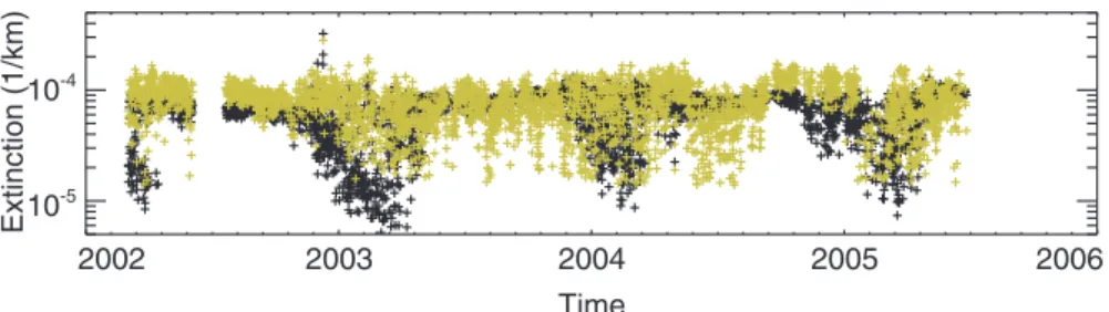
vortex. This is demonstrated in Fig. 1 which shows a time series of northern hemi-sphere SAGE III and POAM III 1020 nm aerosol extinction measurements at 18 km. SAGE III observes many more low aerosol extinction coefficient values (>5×105km−1) during winter months (particularly in the winter of 2002/2003) than does POAM III while conversely showing much less variability during the summer months. Nominally, 15

smaller aerosol extinction coefficients within the polar vortices compared to mid-latitude values is a well known phenomena (Kent el al., 1985; Curtius et al., 2005; Thomason and Poole, 1993) that has been taken into account in PSC identification schemes (e.g., Poole and Pitts, 1994).

To facilitate the use of SAGE III measurements in PSC composition studies and illu-20

minate the differences between SAGE III and POAM III we have conducted an exten-sive comparison of multiwavelength extinction measurements by SAGE III and POAM III with observations made by SAGE II (1984–2005). While SAGE III and SAGE II are more similar to each other than to POAM III, they also have significant differences in hardware configuration and operation. In addition, the SAGE III and SAGE II algorithms 25

that produce the data products including aerosol extinction coefficient, while following similar approaches, are also distinct and have minimal common software. Thus, we do not believe that there is any inherent predilection for the two SAGE instruments to agree at the expense of POAM III and that comparison of these three instruments will

(6)

ACPD

6, 11357–11389, 2006

Full Screen / Esc

EGU provide insight into the source of reported disagreements. Matching SAGE II events to

SAGE III and POAM III is a non-trivial task since SAGE II is in an inclined orbit and, as a result, makes relatively few observations at high latitudes particularly in winter. However, by combining such coincidences over the three winters in which data from all 3 instruments are available (2002/2003 through 2004/2005) and using potential vortic-5

ity as a spatial coordinate rather than latitude, we find roughly 200 co-incidences for SAGE III and SAGE II and roughly 100 co-incidences for POAM III and SAGE II. Herein, we will describe the three instruments and highlight where they and their processing algorithms are different. We then show the results of the data intercomparisons and discuss the results.

10

2 Instrument and algorithm descriptions

All three instruments are solar occultation devices and share the fundamental strengths and weaknesses of this approach. The instruments observe the change in the appar-ent brightness of the Sun as it is obscured (or “occulted”) by the Earth’s atmosphere during each sunrise and sunset encountered by spacecraft or about 30 times per day. 15

A line-of-sight (LOS) transmission is computed by dividing the observed through-the-atmosphere brightness by a value measured above the through-the-atmosphere. By measuring the LOS transmission at multiple wavelengths it is possible to produce profiles of gas species such as ozone, NO₂, and water vapor as well as the spectral dependence of aerosol extinction coefficient. The occultation method is well suited to stratospheric 20

applications where the optical depths of these species are low and where the horizon-tal scale of variability is large since the horizonhorizon-tal scale of the measurements is on the order of hundreds of kilometers and sampling is sparse (Thomason et al., 2003). SAGE III uses 87 channels between 290 and 1540 nm to produce profiles of ozone, NO2, water vapor, temperature, and aerosol extinction coefficient at the 9 wavelengths

25

shown in Table 1 (SAGE III ATBD, 2002). POAM III uses 9 channels between 354 and 1018 nm to produce profiles of ozone, NO2, and water vapor as well as aerosol

(7)

ACPD

6, 11357–11389, 2006

Full Screen / Esc

EGU extinction at the 6 wavelengths shown in Table 1 (Lumpe et al., 2002). SAGE II is the

least complex of these instruments with only 7 channels from which ozone, NO2, wa-ter vapor and aerosol extinction coefficient at 4 wavelengths are produced (Chu et al., 1989; Thomason et al., 2000). We will limit our discussion to the current releases for all instruments: SAGE III (Version 3), POAM III (Version 4), and SAGE II (Version 6.2). In 5

addition, since all three instruments make aerosol extinction coefficient measurements near 1020 nm and 450 nm, we will focus on these common measurements.

In addition to the differences in the number of channels, there are other differences in how the instruments operate. For instance, SAGE II and SAGE III instruments use a mirror to scan across the Sun normal to the horizon continuously during an event. 10

The spacecraft ephemeris and the times of crossing the Sun edges form the basis for determining the altitude of the on-Sun measurements. In the lower atmosphere, where the lower edge of the Sun may be totally obscured, the time of crossing the upper Sun edge and the measured mirror scan rate is used for altitude registration. On the other hand, POAM III stares at the center of brightness of the Sun and uses a combina-15

tion of a molecular density profile derived mostly from the 354 nm channel and an a priori density profile derived from Met Office (MO) data (above ∼26 km) and absolute instrument–based pointing (below ∼26 km). Generally, the physical center and the cen-ter of brightness are the same. However, for Sun positions below ∼40 km, the cencen-ter of brightness moves to an apparently higher position on the Sun due to the effects of 20

refraction and the opacity of the atmosphere. As a result, the retrieval process detects and accounts for this shift and uses an exoatmospheric Sun brightness for the new position. Thus all three instruments are dependent on knowledge of a Sun position-dependent exoatmospheric Sun brightness curve to produce transmission profiles from the measured signals. The field of view of the instruments are 0.5 by 1.5 arc minutes 25

for SAGE III, 0.5 by 5 arc minutes for SAGE II, and 0.8 by 48 arc minutes for POAM III (the unrefracted Sun is 30 arc minutes wide) where the first number denotes the verti-cal field of view and is a key parameter in defining the vertiverti-cal resolution. POAM III has a slightly coarser vertical resolution than the SAGE instruments but this should not be

(8)

ACPD

6, 11357–11389, 2006

Full Screen / Esc

EGU relevant to the following discussions.

SAGE III and SAGE II use a similar approach for the conversion of the measured LOS transmission profiles to LOS product profiles. The effects of molecular scattering are computed using temperature and pressure profiles obtained from the National Center for Environmental Prediction (NCEP). The remaining optical depth (log(transmission)) 5

is separated into contributions by gas species and aerosol using a least squares ap-proach (Chu et al., 1989; Thomason et al., 2000). For SAGE II, the contributions of aerosol in nominal gas channels at 448 (NO₂) and 600 nm (ozone) are approximated as linear combinations of the aerosol LOS optical depth at 452, 525, and 1020 nm where the coefficients for these relationships have been derived based on the relationship 10

predict by single mode log-normal size distributions for sulfate aerosol at stratospheric temperatures (Thomason et al., 2001). The aerosol contribution at 386 nm and in the water vapor channel are computed after the primary processing. SAGE III uses a multi-linear regression (MLR) technique with the twenty 1-nm NO₂ wide channels between 430 and 450 nm and the ten 7-nm wide ozone channels between 560 and 630 nm. The 15

LOS aerosol contribution is produced as a residual following the subtraction of the con-tributions from other components. These include the a priori molecular density profile (from NCEP) and the retrieved ozone and NO2values as well as the contribution of wa-ter vapor (where appropriate) that is retrieved using a non-linear least squares method prior to the application of the MLR technique. Since there is essentially no contribution 20

by ozone at 1020 nm, this channel for both SAGE III and SAGE II is only dependent on the measured transmission and the a priori molecular density profile.

POAM III uses an optimal estimation technique that simultaneously solves for the target gas species and the coefficients to an empirical function that accounts for the effects of aerosol. In this model, aerosol LOS optical depth, δi, is given by

25

δ_i _{= µ}_o_{+ µ}₁κ_i _{+ µ}₂κ_i2, (1) where the µ_j are the effective aerosol coefficients retrieved in the algorithm, and κi ≡ ln(λi), with λi being the central wavelength of channel i. This relationship has been

(9)

ACPD

6, 11357–11389, 2006

Full Screen / Esc

EGU found to be an adequate representation of the spectral dependence predicted by

strato-spheric aerosol models (Lumpe et al., 2002). In describing the previous version (Ver-sion 3), Lumpe et al. (2002) found that the aerosol extinction coefficient at 442 nm is not highly coupled to the extinction at other wavelengths while the value at 1020 nm is significantly coupled to values measured at 779 and 920 nm at all altitudes and to 5

shorter wavelengths above 20 km. For all three instruments, species are separated using LOS values, and those profiles are subsequently “peeled” to the vertical data product profiles.

Randall et al. (2001) compared version 3.0 POAM III aerosol extinction to version 6.0 SAGE II data. They showed that at 1 µm the instruments agreed to within ±30% from 10

10–22 km, but that there was significantly more variability in the POAM measurements. Both the SAGE II and POAM III algorithms have been improved since then; analogous comparisons with the newer versions (not shown) show agreement to within ±10% at 1 µm from 15–24 km, with larger disagreements (±30%) down to 11 km. Substantial variability in the POAM data remains, however, even in the version 4.0 POAM retrievals. 15

The precision at 450 nm was similar between the two instruments, but systematic bi-ases existed that were attributed to problems with the v6.0 SAGE II retrieval algorithm. These problems have been fixed in the version 6.2 algorithm used here, and compar-isons of POAM III data in the northern hemisphere with the newer retrievals agree to within ±20% from 13–21 km, increasing to ±30–40% above and below this range. 20

3 Comparisons

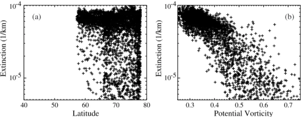
Figure 2 shows the distribution of SAGE III 1020-nm extinction coefficient measure-ments at 18 km north of 45◦_{N for the winters of 2002/2003 to 2004/2005. In frame (a),} the data is plotted as a function of latitude and in frame (b) it is plotted as a function of Ertel potential vorticity (PV) expressed in units of km2s−1kg−1 times 104. SAGE III 25

and SAGE II auxiliary data sets which contain PV, equivalent latitude and other dynam-ical information have been produced by Gloria Manney (Manney et al., 2001) using

(10)

ACPD

6, 11357–11389, 2006

Full Screen / Esc

EGU National Centers for Environmental Prediction (NCEP) analyses and are available at

ftp://mls.jpl.nasa.gov/pub/outgoing/manney. It is clear that the use of PV greatly in-creases the organization of the distribution and illustrates the strength of using this coordinate particularly in the vicinity of the Arctic and Antarctic vortex. As a result, we use time, longitude, altitude, and PV as a coordinates for determining coincidences. 5

Since, as previously noted, there are relatively few opportunities to match SAGE II events in the wintertime Arctic, we found that we needed to use relatively broad match criteria to maximize the number of coincident events. Thus the noise in the matches is likely larger than would be observed with tighter match criteria due to actual geophysi-cal variability. We used identigeophysi-cal altitudes, ±1 day, ±24◦longitude, and ±5% of the PV 10

range observed in the SAGE II data. This latter value is very roughly the equivalent of a 2◦ range in latitude. Since, as will be shown below, all three instruments have roughly the same range in potential vorticity, the opportunity exists to match events for the entire domain of PV. We find some coincidences by these criteria where the latitude difference approaches 10◦. Including these points increased the standard de-15

viation of the comparisons but had little impact on the mean values. As a compromise between the increasing the number of coincidences by opening the coincidence win-dow and decreasing variance by restricting spatial differences, we also include a limit of 5◦difference in latitude. We also eliminated all coincidences where relative errors are greater than 75% and where 1020-nm extinctions values are greater than 4×10−4_km−1

20

and temperatures are less than 200 K as a first cut at removing PSCs. The value used for the relative error limit made virtually no difference in the quality and quantity of matches except above 22 km where significant numbers of POAM III events are elim-inated by a criterion more restrictive than that required by the SAGE instruments. As reported by Lumpe et al. (2002) POAM III extinction measurements report significantly 25

larger uncertainties, particularly at 1020 nm, than those reported in associated with either SAGE data set.

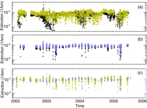
Figure 3 shows the match time history for matching SAGE III and POAM III (a), SAGE III and SAGE II (b), and POAM III and SAGE II (c) coincidences at 18 km using

(11)

ACPD

6, 11357–11389, 2006

Full Screen / Esc

EGU the above match criteria. Clearly Fig. 3a is very similar to Fig. 1 and reflects the

sim-ilarity in sampling that POAM III and SAGE III have in the Northern Hemisphere. At the same time, the differences between SAGE III and POAM III are unchanged by the more robust matching criteria reinforcing the idea that the differences are in fact real differences. On the other hand, the matched SAGE III and SAGE II events, as shown in 5

Fig. 3b, demonstrate a strong qualitative agreement with fewer though still substantial number of matches. Both show a tight clustering during most of the year with some scatter toward lower values in the winter. In Fig. 3c, the matched POAM III and SAGE II events appear similar to the POAM III-SAGE III comparisons shown in Fig. 3a. Here, the POAM III data show greater variability than the SAGE II at all times particularly in 10

the summer of 2003. This is consistent with the POAM II validation results of Randall et al. (2001). The late winter POAM III data show a similar scatter toward lower values as SAGE II that may be consistent with that observed between SAGE III and SAGE II. Figure 4 shows the same analysis except using the measurement channels located near 450 nm. For this set of measurements, the variability of the three data sets is 15

far more consistent than is found for the 1020-nm comparisons. There are systematic differences between the three data sets but all show low variability during the summer and a substantial expansion of the aerosol extinction coefficient domain toward lower values during the winter months. All three data sets reach similar minimum values of 450-nm extinction during the winter periods, around 10−4_km−1_{. This is in contrast to}

20

the comparisons at 1020 nm, where particularly during the 2002–2003 winter minimum POAM III extinction values were significantly higher than from SAGE III.

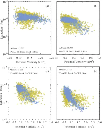
Since our goal is to verify SAGE III’s suitability for PSC studies, we now take a closer look at the matches that occur during the Arctic winter (January–March; 2003–2005) at both 1020 and 450 nm including the extinction or “color” ratios since they play such a 25

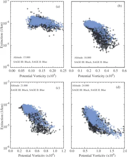
crucial role in PSC type determination. Figures 5 and 6 show a winter-only comparison of 1020-nm aerosol extinction coefficients as a function of PV. In Fig. 5, we show the distribution of SAGE III and SAGE II 1020-nm extinction at 15, 18, 21, and 24 km as a function of PV for the three focus winters. Given the differences in sampling locations,

(12)

ACPD

6, 11357–11389, 2006

Full Screen / Esc

EGU times of measurements, and the mixture of years, some variation in the ensemble of

extinctions is expected. There is no matching of events in this case. Nonetheless we see a similar distribution of values for two instruments though SAGE II has significantly fewer measurements at high PV values than does SAGE III. Other than the 15 km altitude, we observe a significant negative tilt in the aerosol extinction dependence on 5

PV. For instance, the mean value drops by nearly an order of magnitude across the domain of PV. Figure 6 shows the same comparisons for POAM III and SAGE II (the same set of points shown in Fig. 5). POAM III shows also show a tilt with PV but, as would be expected from Fig. 3, with a much larger variation in extinction coefficient at all values of PV. As a result, POAM III 1020-nm extinction coefficients are more weakly 10

correlated with PV than either SAGE II or SAGE III. Since POAM III uses a different PV source than SAGE II/III, it is possible that differences between the PV products could produce an apparently noisy outcome for POAM III. This does not seem likely to be the sole factor since the POAM III summer data still show (shown in Fig. 3) far more variation in extinction coefficient than either SAGE instrument in a period with much 15

weaker PV gradients.

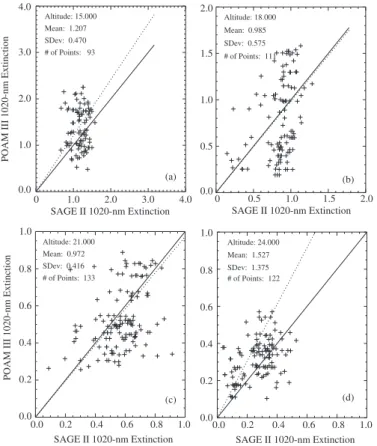
Figure 7 shows the scatter of SAGE III versus SAGE II 1020-nm extinction coefficient limited to data pairs that satisfy our match criteria. We perform our statistical averaging on the ratio, r, of the data pairs as given by

r = ki(λ)

k_SAGEII(λ) (2)

20

where k_i(λ) is the aerosol extinction coefficient at wavelength λ for either SAGE III or

POAM III and kSAGEII(λ) is the corresponding aerosol extinction coefficient for SAGE II. We use the ratio rather than absolute values to even out the importance of the low values (that are of particular interest) with the large values that would otherwise dom-inate the statistical calculations. In these figures, we find that the 1020-nm data from 25

SAGE III and SAGE II are well correlated with a mean of r between 0.83 and 0.90 or a mean difference between –17 and –10%. These values are consistent with the previ-ously reported bias of up to 20% between SAGE III and SAGE II (Thomason and Taha,

(13)

ACPD

6, 11357–11389, 2006

Full Screen / Esc

EGU 2003). The ratio standard deviation values run between 0.15 and 0.35 for roughly 200

matches. Each of the scatter plots shows a fairly tidy primary cluster with a noisier tail toward lower extinction values. The correlation coefficient, R, (the linear Pearson correlation coefficient) between these data sets varies between 0.3 and 0.7. An in-crease in the noise of the matches is not unexpected due to the lower extinction values 5

and imperfect matching of events using PV in regions with apparently high variability in extinction. Nonetheless, it is clear that the occurrence of low extinction measured by one instrument is an indicator of low extinction for the other instrument and the overall domain of extinction coefficient measured by the two instruments is very similar. There are some indications of an increased bias between the two instruments at the lowest 10

extinctions with SAGE III more than 20% less than SAGE II values. However, the noise in the matches makes it difficult to assert this with any certainty. Figure 8 shows the scatter of the approximately 100 matches between POAM III and SAGE II. Here, the mean of the ratios varies from 0.92 to 1.5 with standard deviations of 0.38 to 1.37 or about twice that found between the SAGE instruments. In this figure, while on average 15

the agreement is fairly good, correlation between the data sets is poor particularly be-low 20 km. The correlation coefficient is between 0.0 and 0.5 increasing toward higher altitudes.

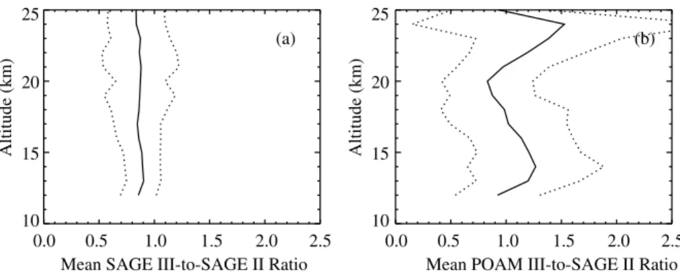
Figure 9 shows a summary of the 1020 nm comparison as a function for height for the SAGE III to SAGE II comparison and the POAM III to SAGE II comparison. We 20

find that the SAGE III and SAGE II comparison has a consistent bias of ∼15% that increases slightly with altitude. The standard deviation of the ratio also shows an in-crease with altitude going from 15% to near 35%. The POAM III to SAGE II profile shows greater structure but averages to a similar bias (though in the opposite sense) to the SAGE III/SAGE II analysis. In this comparison, the standard deviation varies 25

between 40% and 140% over the depth of the profile.

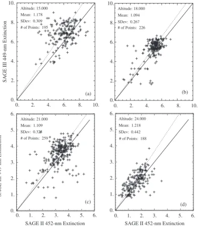
Figures 10 and 11 are complementary to Figs. 7 and 8 for the comparisons at short wavelengths. Since the wavelengths are not the same for these wavelength channels, we expect some differences simply due to the wavelength dependence of aerosol

(14)

ex-ACPD

6, 11357–11389, 2006

Full Screen / Esc

EGU tinction coefficient. For the SAGE III and SAGE II pair (449 and 452 nm), this could be

as large as 2% while for POAM III and SAGE II (442 and 452 nm), it could be as large as 5%. Just by eye it is clear that both comparisons are noisier than at 1020 nm. This is expected since the shorter wavelengths are more strongly influenced by molecular scatter and absorption by gases. As observed for the 1020-nm comparison, the SAGE 5

III and SAGE II comparison shows little variation with altitude. The mean ratio varies from 1.08 to 1.22, the standard deviation is between 0.24 and 0.62, and the correlation coefficient is between 0.24 and 0.72, where all generally increase with altitude. On the other hand, we find that the correspondence between POAM III and SAGE II is better for this pair than at 1020 nm. The mean has a similar range of 0.95 to 1.52 but 10

the standard deviation is between 0.27 and 0.55 or about 2/3 of that for the 1020-nm comparison and very similar to that found for the SAGE III/SAGE II short wavelength comparison. In addition, above 18 km, the correlation coefficient is similar to or larger than the correlation between SAGE III and SAGE II measurements and is consistently greater than 0.5. On the other hand, below 18 km the correlation coefficient between 15

POAM II and SAGE II is close to zero.

The short wavelength summary is shown in Fig. 12. As with the 1020-nm compari-son, the SAGE III and SAGE II short wavelength comparison is consistent with altitude with a bias between 10 and 20% and a the standard deviation between 25 and 60%. The POAM III/SAGE II comparison is significantly better behaved than the 1020-nm 20

comparison. While the mean is similar (ranging from 0.95 to 1.5 over the profile), the standard deviations are much less than at 1020 nm and vary from 27 to 55%.

Since the wavelength ratio is such an important component of the ability to infer PSC composition type, we have also compared the ∼450 to 1020-nm aerosol extinction coefficient color ratios for the two instruments where the color ratio, r, is given by 25

r ₌ ki(450 nm) k_i(1020 nm)×

k_SAGEII(1020 nm)

k_SAGEII(452 nm) , (3)

where the “i ” subscript denotes the either the SAGE III or POAM III instruments. Fig-ure 13 shows the results of this analysis for both SAGE III and POAM III at 18 km;

(15)

ACPD

6, 11357–11389, 2006

Full Screen / Esc

EGU these results are typical of what is seen at between 15 and 25 km. The results are

summarized in Fig. 14. For SAGE III, the mean of the ratio of the extinction ratios is nearly constant at 1.3 below 21 km and increases above that altitude to near 1.5 at 25 km. Similarly the standard deviation is nearly constant below 21 km at a value of 0.2 and increases above that altitude to 0.5. While the mean value of the color ratio can 5

be inferred from previous figures, the low standard deviation in the ratio is less obvious and arises out of the fact that the errors in the extinction coefficient measurements as a function of wavelength are highly correlated for both instruments and do not fluctu-ate independently (Kent et al., 2006). The low dynamic range in the ratio (only about ±15%) leads to relatively low correlation coefficient values that lie near 0.3 over the 10

entire depth of the profile. The POAM III to SAGE II comparisons can also be inferred from the results shown above. There is substantial structure in the altitude profiles of the individual comparisons shown in Figs. 9 and 12, which leads to the structure observed in Fig. 14. In this case, the ratio varies from 1.7 at 12 km to around 0.83 at 23 km and is generally near 1.5 between 15 and 20 km. As shown above, the POAM 15

III extinction at both 1 µm and 450 nm is on average biased high compared to SAGE II, with a larger bias at 450 nm. This leads to the generally positive bias in the wave-length ratio seen in Fig. 14. The large scatter in color ratio between these instruments is clearly seen in Fig. 13 where the range for POAM III ranges from values of about 2 to nearly 20 while SAGE II varies from 4 to 9 and SAGE III varies between 5.5 and 9 20

with a few points between 10 and 15. This results primarily from the large variability in the POAM III 1-µm measurements, as described previously (Randall et al., 2001). Not surprisingly, the correlation between SAGE II and POAM III color ratios is for all intents and purposes zero.

It is interesting to note that both the SAGE III and POAM III instruments show larger 25

color ratios than the SAGE II instrument. This is consistent with comparisons (not shown) between the three instruments for more standard coincidence criteria (e.g., ±24 h, 500 km). These comparisons comprise more than 2000 SAGE III/POAM III co-incidences (many during the winter) and more than 300 SAGE III/SAGE II coco-incidences

(16)

ACPD

6, 11357–11389, 2006

Full Screen / Esc

EGU (none during the winter). These comparisons reveal that the color ratio for SAGE III is

20–30% higher than the color ratio for SAGE II, from 10–22 km. This results from the fact that SAGE III extinction at 450 nm is ∼10–15% higher than SAGE II, whereas it is 10–15% lower at 1 µm. Given the very low background levels of aerosol extinction that persisted throughout the lifetime of SAGE III, this is quite reasonable agreement. As 5

expected from the more variable POAM measurements at 1 µm, the color ratio com-parison for SAGE III vs. POAM III shows more structure, but on average is within ±20% from ∼13–21 km. In this altitude range SAGE III and POAM III extinctions at 450 nm are within ±15%, while at 1 µm POAM III is higher than SAGE III by 20–30% (increasing to 40–60% below 15 km).

10

We now return to the original question raised by the results of Russell et al. (2004) and shown in Fig. 1: are the differences between POAM III and SAGE III aerosol ex-tinction at 1 µm that are most obvious in the 2002–2003 winter indicative of a problem in the SAGE III data? We conclude that based on comparisons of both the SAGE III and POAM III data sets to a common standard, SAGE II, we have no evidence to sug-15

gest that there is any more error in the SAGE III data than in the other data sets. The precision of the SAGE III 1-µm data is significantly higher than that of POAM III, which lends credibility to the SAGE III retrievals. On average, as seen from Fig. 14, the color ratio of SAGE III is intermediate between that of SAGE II and POAM III, another point that suggests the SAGE III measurements are not significantly in error. In addition, 20

the lack of an appreciable altitude dependence in the relationship between the 1020 and 450-nm measurements by SAGE III and SAGE II (Figs. 9a and 12a) suggests that these measurements are robust since most known sources of bias in these measure-ments are both strongly wavelength and altitude dependent (Thomason et al., 20061). Conversely, SAGE III extinctions at 1 µm are lower than both SAGE II and POAM III, 25

so this could point to a low bias in the SAGE III 1-µm extinction measurements that

1

Thomason L. W., Burton, S. P., Luo, B.-P., and Peter, T.: SAGE II Measurements of Strato-spheric Aerosol Properties at Non-Volcanic Levels, Atmos. Chem. Phys. Discuss., in prepara-tion, 2006.

(17)

ACPD

6, 11357–11389, 2006

Full Screen / Esc

EGU might be at least partly responsible for the low values in winter. At this time, however,

the causes of the overall biases between these three instruments are not understood, and errors cannot be definitively attributed to one instrument instead of another.

4 Summary and conclusions

Based on this analysis, we find that the SAGE III data at both 1020 and 449 nm is 5

reliable over a broad range of aerosol extinction values and suitable for use in PSC studies. Both of these channels show systematic bias relative to the SAGE II values that are nearly constant from 12 to 25 km, but in opposite directions. In addition, the color ratios for these instruments, while reflecting the individual biases, remains highly robust and are extremely consistent as a function of altitude. We have not attempted 10

to diagnose the source of the differences between the two SAGE instruments. Differ-ences between POAM III and SAGE II, particularly at 1020 nm, vary significantly with altitude, but the overall magnitude of the differences is similar to that between SAGE III and SAGE II. POAM III measurements are significantly less noisy at 450 nm than at 1 µm, so the comparisons with SAGE II at the shorter wavelengths are better behaved. 15

As has been previously reported, the POAM III aerosol extinction data at 1 µm is sig-nificantly noisier than the data from either SAGE instrument and it is possible that this contributes to reported disagreements (Russell et al., 2005). These disagreements might also arise in part from the small systematic low bias, currently not understood, that is observed between SAGE III and both SAGE II and POAM at 1-µm. In any 20

case, we conclude that based on the above analysis that, beyond the modest biases reported here, there is no reason to believe that the SAGE III data is pathologically biased low within the polar vortex or that the low extinctions recorded by the instrument are anything but the product of geophysical processes.

Acknowledgements. The authors would like to thank G. Manney of JPL for providing a wealth

25

of auxiliary data for SAGE II and SAGE III including the potential vorticity data used in this paper.

(18)

ACPD

6, 11357–11389, 2006

Full Screen / Esc

EGU

References

Chu, W. P., McCormick, M. P., Lenoble, J., Brogniez, C., and Pruvost, P.: SAGE II inversion algorithm, J. Geophys. Res., 94, 8339–8351, 1989.

Curtius, J., Weigel, R., V ¨ossing, H.-J., Wernli, H., Werner, A., Volk, C.-M., Konopka, P., Krebs-bach, M., Schiller, C., Roiger, A., Schlager, H., Dreilling, V., and Borrmann, S.: Observations 5

of meteoric material and implications for aerosol nucleation in the winter Arctic lower strato-sphere derived from in situ particle measurements, Atmos. Chem. Phys., 5, 3053–3069, 2005.

Fromm, M., Alfred, J., and Pitts, M.: A unified, long-term, high-latitude stratospheric aerosol and cloud database using SAM II, SAGE II, and POAM II/III data: algorithm description, database 10

definition, and climatology, J. Geophys. Res., 108, 4366, doi:10.1029/2002JD002772, 2003. Kent, G. S., Trepte, C. R., Farrukh, U. O., and McCormick, M. P.: Variation in the stratospheric

aerosol associated with the north cyclonic polar vortex as measured by the SAM II satellite sensor, J. Atmos. Sci., 42, 1536–1551, 1985.

Lumpe, J. D., Bevilacqua, R. M., Hoppel, K. W., and Randall, C. E.: POAM III retrieval algorithm 15

and error analysis, J. Geophys. Res., 107(D21), 4575, doi:10.1029/2002JD002137, 2002. Manney, G. L., Michelsen, H. A., Bevilacqua, R. M., Gunson, M. R., Irion, F. W., Livesey, N. J.,

Oberheide, J., Riese, M., Russell III, J. M., Toon, G. C., and Zawodny, J. M.: Comparison of satellite ozone observations in coincident air masses in early November 1994, J. Geophys. Res., 106, 9923–9943, 2001.

20

McCormick, M. P., Chu, W. P., Grams, G. W., Hamill, P., Herman, B. M., McMaster, L. R., Pepin, T. J., Russell, P. B., Steele, H. M,. and Swissler, T. J.: High-latitude stratospheric aerosols measured by the SAM II satellite system in 1978 and 1979, Science, 214, 328–331, 1981. Poole, L. R. and Pitts, M. C.: Polar stratospheric cloud climatology based on Stratospheric

Aerosol Measurement II observations from 1978 to 1989, J. Geophys. Res., 99, 13 083– 25

13 089, 1994.

Randall, C. E., Bevilacqua, R. M., Lumpe, J. D., and Hoppel, K. W.: Validation of POAM III aerosols: Comparison to SAGE II and HALOE, J. Geophys. Res., 106(D21), 27 525–27 536, 2001.

Russell, P., Livingston, J., Schmid, B., Eilers, J., Kolyer, R., Redemann, J., Ramirez, S., Yee, 30

J.-H., Swartz, W., Shetter, R., Trepte, C., Risley Jr., A., Wenny, B., Zawodny, J., Chu, W., Pitts, M., Lumpe, J., Fromm, M., Randall, C., Hoppel, K., and Bevilacqua, R.: Aerosol optical

(19)

ACPD

6, 11357–11389, 2006

Full Screen / Esc

EGU depth measurements by airborne sun photometer in SOLVE II: Comparisons to SAGE III,

POAM III and airborne spectrometer measurements, Atmos. Chem. Phys., 5, 1311–1339, 2005.

SAGE III Algorithm Theoretical Basis Document: Solar and Lunar Algorithm, LaRC 475-00-108, Version 2.1, 26 March 2002.

5

Strawa, A. W., Drdla, K., Fromm, M., Pueschel, R. F., Hoppel, K. W., Browell, E. V., Hamill, P., and Dempsey, D. P.: Discriminating Types Ia and Ib polar stratospheric clouds in POAM satellite data, J. Geophys. Res., 107(D20), 8291, doi:10.1029/2001JD000458, 2002. Thomason, L. W. and Poole, L. R.: Use of stratospheric aerosol properties as diagnostics of

Antarctic vortex processes, J. Geophys. Res., 98, 23 003–23 012, 1993. 10

Thomason, L. W., Zawodny, J. M., Burton, S. P., and Iyer, N.: The SAGE II Algorithm: Ver-sion 6.0 and On-going Developments, 8th Scientific Assembly of International Association of Meteorology and Atmospheric Sciences, Innsbruck Austria, July 10–18, 2001.

Thomason, L. W. and Taha, G.: SAGE III Aerosol Extinction Measurements: Initial Results, Geophys. Res. Lett., 30, 1631, doi:10.1029/2003GL017317, 2003.

(20)

ACPD

6, 11357–11389, 2006

Full Screen / Esc

EGU

Table 1. Aerosol extinction coefficient wavelengths for SAGE II, SAGE III, and POAM III in

nanometers. (check numbers).

SAGE II SAGE III POAM III

386 385 354 452 449 442 525 521 600 1020 600 779 676 920 755 1020 868 1020 1540

(21)

ACPD

6, 11357–11389, 2006

Full Screen / Esc

Printer-friendly Version Interactive Discussion EGU 2002 2003 2004 2005 2006 Time 10-5 10-4 Extinction (1/km)

Fig. 1. This figure shows the 18-km, 1020-nm aerosol extinction coefficient measured by

SAGE III (black) and POAM III (gold) in the Northern Hemisphere. Note that this figure shows all observations by each instrument with no matching requirement.

(22)

ACPD

6, 11357–11389, 2006

Full Screen / Esc

Printer-friendly Version Interactive Discussion EGU 40 50 60 70 80 Latitude 10-5 10-4 Extinction (1/km) 0.3 0.4 0.5 0.6 0.7 Potential Vorticity 10-5 10-4 Extinction (1/km) (a) (b)

Fig. 2. This figure depicts a comparison of the distribution of 1020-nm aerosol extinction

coeffi-cient from SAGE III in January through March of 2003 through 2005 at 20 km. Frame (a) shows the distribution as a function of latitude while frame (b) shows the distribution as a function of potential vorticity in units of km2s−1_kg−1_{times 10}4

(23)

ACPD

6, 11357–11389, 2006

Full Screen / Esc

Printer-friendly Version Interactive Discussion EGU 2002 2003 2004 2005 2006 Time 10-5 10-4 Extinction (1/km) 10-5 10-4 Extinction (1/km) 10-5 10-4 Extinction (1/km) (a) (b) (c)

Fig. 3. This figure shows 18 km, 1020-nm aerosol extinction coefficient measured by SAGE III,

SAGE II, and POAM II using the match requirements described in the text. Frame (a) shows SAGE III (black) matched with POAM III (gold); frame (b) shows SAGE III (black) matched with SAGE II (blue); and frame (c) shows POAM III (gold) matched with SAGE II (blue).

(24)

ACPD

6, 11357–11389, 2006

Full Screen / Esc

Printer-friendly Version Interactive Discussion EGU 10-5 10-4 10-3 Extinction (1/km) 10-5 10-4 10-3 Extinction (1/km) 10-5 10-4 10-3 Extinction (1/km) 2002 2003 2004 2005 2006 Time (a) (b) (c)

Fig. 4. This figure shows 18 km, aerosol extinction coefficient near 450-nm as measured by

SAGE III, SAGE II, and POAM II using the match requirements described in the text. Frame

(a) shows POAM III (gold) matched with SAGE III (black); frame (b) shows SAGE III (black)

matched with SAGE II (blue); and frame (c) shows SAGE II (black) matched with POAM III (gold).

(25)

ACPD

6, 11357–11389, 2006

Full Screen / Esc

Printer-friendly Version Interactive Discussion EGU 0.00 0.05 0.10 0.15 0.20 0.25 Potential Vorticity (x104) 10-6 10-5 10-4 10-3 Extinction (1/km) 0.0 0.1 0.2 0.3 0.4 0.5 0.6 Altitude: 18.000

SAGE III: Black, SAGE II: Blue

Potential Vorticity (x104)

0.0 0.2 0.4 0.6 0.8 1.0 1.2

Altitude: 21.000

10-6 10-5 10-4 10-3 Extinction (1/km) Potential Vorticity (x104) 0.0 0.5 1.0 1.5 2.0 Altitude: 24.000

(a) (b)

(c) (d)

Altitude: 15.000

Fig. 5. This figure shows the distribution of 1020-nm aerosol extinction coefficient measured by

SAGE III (black) and SAGE II (blue) at 15 (a), 18 (b), 21 (c), and 24 km (d) for January through March of 2003 through 2005. The plots show all data without any matching requirements.

(26)

ACPD

6, 11357–11389, 2006

Full Screen / Esc

EGU

Altitude: 15.000

POAM III: Black, SAGE II: Blue

10-6 10-5 10-4 10-3 Extinction (1/km) Potential Vorticity (x104) 0.05 0.10 0.15 0.20 0.25 0.1 0.2 0.3 0.4 0.5 0.6 Altitude: 18.000

0.0 0.2 0.4 0.6 0.8 1.0 1.2 1.4

Altitude: 21.000

10-6 10-5 10-4 10-3 Extinction (1/km) Potential Vorticity (x104) 0.0 0.5 1.0 1.5 2.0 2.5 3.0 Altitude: 24.000

(a) (b)

(c) (d)

Fig. 6. This figure shows the distribution of 1020-nm aerosol extinction coefficient measured by

POAM III (gold) and SAGE II (blue) at 15 (a), 18 (b), 21 (c), and 24 km (d) for January through March of 2003 through 2005. The plots show all data without any matching requirements.

(27)

ACPD

6, 11357–11389, 2006

Full Screen / Esc

EGU

SAGE III 1020-nm Extinction

SAGE II 1020-nm Extinction (a) 0 0.5 1.0 1.5 2.0 SAGE II 1020-nm Extinction 0 0.5 1.0 1.5 2.0 Altitude: 15.000 Mean: 0.887 SDev: 0.167 # of Points: 195 Altitude: 18.000 Mean: 0.862 SDev: 0.254 # of Points: 226 0 0.5 1.0 1.5 2.0 SAGE II 1020-nm Extinction 0 0.5 1.0 1.5 2.0 Altitude: 21.000 Mean: 0.880 SDev: 0.342 # of Points: 259 1.0 0.8 0.6 0.4 0.2 0.0 0.0 0.2 0.4 0.6 0.8 1.0 Altitude: 24.000 Mean: 0.837 SDev: 0.262 # of Points: 188 1.0 0.8 0.6 0.4 0.2 0.0 SAGE II 1020-nm Extinction 0.0 0.2 0.4 0.6 0.8 1.0 (b) (c) (d)

Fig. 7. This figure shows the relationship between SAGE III and SAGE II 1020-nm aerosol

extinction coefficient pairs matched using the criteria described in the text for 15 (a), 18 (b), 21 (c), and 24 km (d). All extinctions are multiplied by 104. The mean statistics shown were computed using the ratio defined in Eq. (1). The dotted line is the least squares fit for the data (constrained to pass through the origin) and the solid line has a slope of 1.

(28)

ACPD

6, 11357–11389, 2006

Full Screen / Esc

EGU

POAM III 1020-nm Extinction

SAGE II 1020-nm Extinction (a) 0 1.0 2.0 3.0 4.0 SAGE II 1020-nm Extinction 0.0 1.0 2.0 3.0 4.0 0 0.5 1.0 1.5 2.0 SAGE II 1020-nm Extinction 0.0 0.5 1.0 1.5 2.0 1.0 0.8 0.6 0.4 0.2 0.0 0.0 0.2 0.4 0.6 0.8 1.0 1.0 0.8 0.6 0.4 0.2 0.0 SAGE II 1020-nm Extinction 0.0 0.2 0.4 0.6 0.8 1.0 (b) (c) (d) Altitude: 24.000 Mean: 1.527 SDev: 1.375 # of Points: 122 Altitude: 15.000 Mean: 1.207 SDev: 0.470 # of Points: 93 Altitude: 18.000 Mean: 0.985 SDev: 0.575 # of Points: 111 Altitude: 21.000 Mean: 0.972 SDev: 0.416 # of Points: 133

Fig. 8. This figure shows the relationship between SAGE II and POAM III 1020-nm aerosol

extinction coefficient pairs matched using the criteria described in the text for 15 (a), 18 (b), 21 (c), and 24 km (d). All extinctions are multiplied by 104. The mean statistics shown were computed using the ratio defined in Eq. (1). The dotted line is the least squares fit for the data (constrained to pass through the origin) and the solid line has a slope of 1.

(29)

ACPD

6, 11357–11389, 2006

Full Screen / Esc

EGU

0.0 0.5 1.0 1.5 2.0

Mean SAGE III-to-SAGE II Ratio 10

15 20 25

Altitude (km)

Mean POAM III-to-SAGE II Ratio 10 15 20 25 Altitude (km) (a) (b) 2.5 0.0 0.5 1.0 1.5 2.0 2.5

Fig. 9. (a) Mean profile of the ratio of SAGE III and SAGE II 1020-nm aerosol extinctions

coefficients for the winters of 2003 through 2005. The solid line is the mean while the dotted line is the 1-sigma confidence limits. (b) Same as frame (a) except for POAM III and SAGE II.

(30)

ACPD

6, 11357–11389, 2006

Full Screen / Esc

EGU

SAGE II 452-nm Extinction

SAGE II 452-nm Extinction (a) (b) (d) (c) Altitude: 15.000 Mean: 1.178 SDev: 0.309 # of Points: 195 10. 8. 6. 4. 2. 0. 2. 0. 4. 6. 8. 10. Altitude: 18.000 Mean: 1.094 SDev: 0.267 # of Points: 226 2. 0. 4. 6. 8. 10. 10. 8. 6. 4. 2. 0. Altitude: 21.000 Mean: 1.109 SDev: 0.325 # of Points: 259 6. 5. 4. 3. 2. 1. 0. 0. 1. 2. 3. 4. 5. 6. Altitude: 24.000 Mean: 1.218 SDev: 0.442 # of Points: 188 6. 5. 4. 3. 2. 1. 0. 0. 1. 2. 3. 4. 5. 6.

Fig. 10. This figure shows the relationship between SAGE III and SAGE II short wavelength

aerosol extinction coefficient pairs (449 and 452 nm) matched using the criteria described in the text for 15 (a), 18 (b), 21 (c), and 24 km (d). All extinctions are multiplied by 104. The mean statistics shown were computed using the ratio defined in Eq. (1). The dotted line is the least squares fit for the data (constrained to pass through the origin) and the solid line has a slope of 1.

(31)

ACPD

6, 11357–11389, 2006

Full Screen / Esc

EGU

SAGE II 452-nm Extinction

SAGE II 452-nm Extinction (a) (b) (d) (c) Altitude: 15.000 Mean: 1.493 SDev: 0.512 # of Points: 98 20. 15. 10. 5. 0. 0. 5. 10. 15. 20. Altitude: 18.000 Mean: 1.220 SDev: 0.414 # of Points: 117 10. 8. 6. 4. 2. 0. 2. 0. 4. 6. 8. 10. Altitude: 21.000 Mean: 1.134 SDev: 0.345 # of Points: 136 6. 5. 4. 3. 2. 1. 0. 0. 1. 2. 3. 4. 5. 6. Altitude: 24.000 Mean: 0.961 SDev: 0.307 # of Points: 113 4. 3. 2. 1. 0. 0. 1. 2. 3. 4.

Fig. 11. This figure shows the relationship between SAGE II and POAM III short wavelength

aerosol extinction coefficient pairs (452 and 442 nm) matched using the criteria described in the text for 15 (a), 18 (b), 21 (c), and 24 km (d). All extinctions are multiplied by 104. The mean statistics shown were computed using the ratio defined in Eq. (1). The dotted line is the least squares fit for the data (constrained to pass through the origin) and the solid line has a slope of 1.

(32)

ACPD

6, 11357–11389, 2006

Full Screen / Esc

EGU

0.0 0.5 1.0 1.5 2.0

Mean SAGE III-to-SAGE II Ratio 10 15 20 25 Altitude (km) 0.0 0.5 1.0 1.5 2.0

Mean POAM III-to-SAGE II Ratio 10 15 20 25 Altitude (km) (a) (b)

Fig. 12. (a) Mean profile of the ratio of SAGE III 449 nm and SAGE II 452-nm aerosol extinctions

coefficients for the winters of 2003 through 2005. The solid line is the mean while the dotted line is the 1-sigma confidence limits. (b) Same as frame (a) except for POAM III 442 nm and SAGE II 452-nm aerosol extinction coefficient.

(33)

ACPD

6, 11357–11389, 2006

Full Screen / Esc

EGU

SAGE II Extinxtion Ratio

SAGE III Extinction Ratio

0 5 10 15 20 SAGE II Extinxtion Ratio 0

5 10 15 20

POAM III Extinction Ratio

(b) 0 5 10 15 20 0 5 10 15 20 (a) Altitude: 18.000 Mean: 1.288 SDev: 0.153 # of Points: 226 Altitude: 18.000 Mean: 1.469 SDev: 0.927 # of Points: 99

Fig. 13. This figure shows the relationship between (a) SAGE III and SAGE II aerosol extinction

coefficient ratio pairs (449 to 1020-nm and 452 to 1020-nm) and (b) POAM III and SAGE II aerosol extinction coefficient ratio pairs (442 to 1020-nm and 452 to 1020-nm) at 18 km matched using the criteria described in the text. The mean statistics shown were computed using the ratio defined in Eq. (2). The dotted line is the least squares fit for the data (constrained to pass through the origin) and the solid line has a slope of 1.

(34)

ACPD

6, 11357–11389, 2006

Full Screen / Esc

EGU 0.0 0.5 1.0 1.5 2.0 2.5

Mean SAGE III-to-SAGE II Ratio 10 15 20 25 Altitude (km) 0.0 0.5 1.0 1.5 2.0 2.5 Mean POAM III-to-SAGE II Ratio 10 15 20 25 Altitude (km) (a) (b)

Fig. 14. (a) Mean profile of the ratio of SAGE III 449 to 1020-nm aerosol extinction ratio and

the SAGE II 452 nm to 1020-nm aerosol extinction ratio for the winters of 2003 through 2005. The solid line is the mean while the dotted line is the 1-sigma confidence limits. (b) Same as frame (a) except for POAM III 442 nm to 1018 nm aerosol extinction ratio and the SAGE II 452 to 1020-nm aerosol extinction ratio.