HAL Id: hal-01554386
https://hal.archives-ouvertes.fr/hal-01554386
Submitted on 3 Jun 2020
HAL is a multi-disciplinary open access
archive for the deposit and dissemination of
sci-entific research documents, whether they are
pub-lished or not. The documents may come from
teaching and research institutions in France or
abroad, or from public or private research centers.
L’archive ouverte pluridisciplinaire HAL, est
destinée au dépôt et à la diffusion de documents
scientifiques de niveau recherche, publiés ou non,
émanant des établissements d’enseignement et de
recherche français ou étrangers, des laboratoires
publics ou privés.
Fermi-LAT Observations of High-energy
Behind-the-limb Solar Flares
M. Ackermann, A. Allafort, L. Baldini, G. Barbiellini, D. Bastieri, R.
Bellazzini, E. Bissaldi, R. Bonino, E. Bottacini, J. Bregeon, et al.
To cite this version:
M. Ackermann, A. Allafort, L. Baldini, G. Barbiellini, D. Bastieri, et al.. Fermi-LAT Observations
of High-energy Behind-the-limb Solar Flares. Astrophys.J., 2017, 835 (2), pp.219.
�10.3847/1538-4357/835/2/219�. �hal-01554386�
Fermi-LAT Observations of High-energy Behind-the-limb Solar Flares
M. Ackermann1, A. Allafort2, L. Baldini3, G. Barbiellini4,5, D. Bastieri6,7, R. Bellazzini8, E. Bissaldi9, R. Bonino10,11, E. Bottacini2, J. Bregeon12, P. Bruel13, R. Buehler1, R. A. Cameron2, M. Caragiulo9,14, P. A. Caraveo15, E. Cavazzuti16, C. Cecchi17,18, E. Charles2, S. Ciprini16,17, F. Costanza9, S. Cutini16,17, F. D’Ammando19,20, F. de Palma9,21, R. Desiante10,22, S. W. Digel2,
N. Di Lalla3, M. Di Mauro2, L. Di Venere9,14, P. S. Drell2, C. Favuzzi9,14, Y. Fukazawa23, P. Fusco9,14, F. Gargano9, N. Giglietto9,14, F. Giordano9,14, M. Giroletti19, I. A. Grenier24, L. Guillemot25,26, S. Guiriec27,50, T. Jogler28, G. Jóhannesson29,30,
L. Kashapova31, S. Krucker32,33, M. Kuss8, G. La Mura7, S. Larsson34,35, L. Latronico10, J. Li36, W. Liu2,37,38, F. Longo4,5, F. Loparco9,14, P. Lubrano17, J. D. Magill39, S. Maldera10, A. Manfreda3, M. N. Mazziotta9, W. Mitthumsiri40, T. Mizuno41, M. E. Monzani2, A. Morselli42, I. V. Moskalenko2, M. Negro10,11, E. Nuss12, T. Ohsugi41, N. Omodei2, E. Orlando2, V. Pal’shin43, D. Paneque44, J. S. Perkins27, M. Pesce-Rollins8, V. Petrosian2, F. Piron12, G. Principe45, S. Rainò9,14, R. Rando6,7, M. Razzano8,51, O. Reimer2,46, F. Rubio da Costa2, C. Sgrò8, D. Simone9, E. J. Siskind47, F. Spada8, G. Spandre8, P. Spinelli9,14, H. Tajima2,48,
J. B. Thayer2, D. F. Torres36,49, E. Troja27,39, and G. Vianello2 1
Deutsches Elektronen Synchrotron DESY, D-15738 Zeuthen, Germany
2
W. W. Hansen Experimental Physics Laboratory, Kavli Institute for Particle Astrophysics and Cosmology, Department of Physics and SLAC National Accelerator Laboratory, Stanford University, Stanford, CA 94305, USA;[email protected],[email protected]
3
Università di Pisa and Istituto Nazionale di Fisica Nucleare, Sezione di Pisa I-56127 Pisa, Italy
4
Istituto Nazionale di Fisica Nucleare, Sezione di Trieste, I-34127 Trieste, Italy
5
Dipartimento di Fisica, Università di Trieste, I-34127 Trieste, Italy
6
Istituto Nazionale di Fisica Nucleare, Sezione di Padova, I-35131 Padova, Italy
7
Dipartimento di Fisica e Astronomia“G. Galilei,” Università di Padova, I-35131 Padova, Italy
8
Istituto Nazionale di Fisica Nucleare, Sezione di Pisa, I-56127 Pisa, Italy;[email protected] 9
Istituto Nazionale di Fisica Nucleare, Sezione di Bari, I-70126 Bari, Italy
10
Istituto Nazionale di Fisica Nucleare, Sezione di Torino, I-10125 Torino, Italy
11
Dipartimento di Fisica, Università degli Studi di Torino, I-10125 Torino, Italy
12
Laboratoire Univers et Particules de Montpellier, Université Montpellier, CNRS/IN2P3, F-34095 Montpellier, France
13Laboratoire Leprince-Ringuet, École polytechnique, CNRS/IN2P3, F-91128 Palaiseau, France 14
Dipartimento di Fisica“M. Merlin” dell’Università e del Politecnico di Bari, I-70126 Bari, Italy
15
INAF-Istituto di Astrofisica Spaziale e Fisica Cosmica Milano, via E. Bassini 15, I-20133 Milano, Italy
16
Agenzia Spaziale Italiana(ASI) Science Data Center, I-00133 Roma, Italy
17
Istituto Nazionale di Fisica Nucleare, Sezione di Perugia, I-06123 Perugia, Italy
18
Dipartimento di Fisica, Università degli Studi di Perugia, I-06123 Perugia, Italy
19
INAF Istituto di Radioastronomia, I-40129 Bologna, Italy
20
Dipartimento di Astronomia, Università di Bologna, I-40127 Bologna, Italy
21
Università Telematica Pegaso, Piazza Trieste e Trento, 48, I-80132 Napoli, Italy
22Università di Udine, I-33100 Udine, Italy 23
Department of Physical Sciences, Hiroshima University, Higashi-Hiroshima, Hiroshima 739-8526, Japan
24
Laboratoire AIM, CEA-IRFU/CNRS/Université Paris Diderot, Service d’Astrophysique, CEA Saclay, F-91191 Gif sur Yvette, France
25
Laboratoire de Physique et Chimie de l’Environnement et de l’Espace—Université d’Orléans/CNRS, F-45071 Orléans Cedex 02, France
26
Station de radioastronomie de Nançay, Observatoire de Paris, CNRS/INSU, F-18330 Nançay, France
27
NASA Goddard Space Flight Center, Greenbelt, MD 20771, USA
28
Friedrich-Alexander-Universität, Erlangen-Nürnberg, Schlossplatz 4, D-91054 Erlangen, Germany
29
Science Institute, University of Iceland, IS-107 Reykjavik, Iceland
30
NORDITA, Roslagstullsbacken 23, SE-106 91 Stockholm, Sweden
31
Institute of Solar-Terrestrial SB RAS, Lermontov st. 126a, 6640333, Irkutsk, Russia
32
University of Applied Sciences and Arts Northwestern Switzerland, CH-5210 Windisch, Switzerland
33Space Science Laboratory, University of California, Berkeley, CA 94720-7450, USA 34
Department of Physics, KTH Royal Institute of Technology, AlbaNova, SE-106 91 Stockholm, Sweden
35
The Oskar Klein Centre for Cosmoparticle Physics, AlbaNova, SE-106 91 Stockholm, Sweden
36
Institute of Space Sciences(IEEC-CSIC), Campus UAB, Carrer de Magrans s/n, E-08193 Barcelona, Spain
37
Bay Area Environmental Research Institute, 625 2nd Street, Suite 209, Petaluma, CA 94952, USA
38
Lockheed Martin Solar and Astrophysics Laboratory, 3251 Hanover Street, Bldg. 252, Palo Alto, CA 94304, USA
39
Department of Physics and Department of Astronomy, University of Maryland, College Park, MD 20742, USA
40
Department of Physics, Faculty of Science, Mahidol University, Bangkok 10400, Thailand
41
Hiroshima Astrophysical Science Center, Hiroshima University, Higashi-Hiroshima, Hiroshima 739-8526, Japan
42Istituto Nazionale di Fisica Nucleare, Sezione di Roma“Tor Vergata,” I-00133 Roma, Italy 43
St. Peterburg, Vedeneeva 2-31, Russia
44
Max-Planck-Institut für Physik, D-80805 München, Germany
45
Erlangen Centre for Astroparticle Physics, D-91058 Erlangen, Germany
46
Institut für Astro- und Teilchenphysik and Institut für Theoretische Physik, Leopold-Franzens-Universität Innsbruck, A-6020 Innsbruck, Austria
47
NYCB Real-Time Computing Inc., Lattingtown, NY 11560-1025, USA
48
Solar-Terrestrial Environment Laboratory, Nagoya University, Nagoya 464-8601, Japan
49
Institució Catalana de Recerca i Estudis Avançats(ICREA), E-08010 Barcelona, Spain
Received 2016 October 13; revised 2016 November 23; accepted 2016 December 31; published 2017 January 31
doi:10.3847/1538-4357/835/2/219
The Astrophysical Journal, 835:219 (13pp), 2017 February 1
50
NASA Postdoctoral Program Fellow, USA.
51
Abstract
We report on the Fermi-LAT detection of high-energy emission from the behind-the-limb(BTL) solar flares that occurred on 2013 October 11, and 2014 January 6 and September 1. The Fermi-LAT observations are associated withflares from active regions originating behind both the eastern and western limbs, as determined by STEREO. All three flares are associated with very fast coronal mass ejections (CMEs) and strong solar energetic particle events. We present updated localizations of the>100 MeV photon emission, hard X-ray (HXR) and EUV images, and broadband spectra from 10 keV to 10 GeV, as well as microwave spectra. We also provide a comparison of the BTL flares detected by Fermi-LAT with three on-disk flares and present a study of some of the significant quantities of these flares as an attempt to better understand the acceleration mechanisms at work during these occulted flares. We interpret the HXR emission to be due to electron bremsstrahlung from a coronal thin-target loop top with the accelerated electron spectra steepening at semirelativistic energies. The>100 MeV gamma-rays are best described by a pion-decay model resulting from the interaction of protons(and other ions) in a thick-target photospheric source. The protons are believed to have been accelerated (to energies >10 GeV) in the CME environment and precipitate down to the photosphere from the downstream side of the CME shock and landed on the front side of the Sun, away from the original flare site and the HXR emission.
Key words: Sun: flares – Sun: X-rays, gamma rays
1. Introduction
Gamma-ray emission from solarflares is generally believed to occur predominantly in compact high-density regions near the photospheric footpoints of magnetic field lines. Observa-tions of gamma-ray emission from flares whose host active regions (ARs) are located behind the visible solar disk pose interesting questions regarding the acceleration sites and mechanism, the transport and interaction points of the accelerated particles during these rare events.
Three behind-the-limb (BTL) flares with emission up to 100 MeV were observed during solar cycles 21 and 22. The first occulted solar flare whose AR was estimated to be 15° behind the western limb was observed on 1989 September 29 by the Gamma-Ray Spectrometer (GRS) on board the Solar Maximum Mission(SMM). Vestrand & Forrest (1993) reported intense gamma-ray line emission in the 1–8 MeV range and a strong 2.223 MeV neutron capture line from this flare. Given the strength of the line emission, it was concluded that a spatially extended component was required in order to explain the observations. The second, detected by PHEBUS on GRANAT(Barat et al. 1994) on 1991 June 1, had intense gamma-ray line emission in the 1–8 MeV range but no neutron capture line, indicating that the emission was of coronal origin. The third occulted flare, detected by PHEBUS, BATSE, and EGRET on 1991 June 30, was an electron-dominatedflare with no detectable line emission but with significant emission up to almost 100 MeV. Vilmer et al. (1999) report that the spectral properties of this flare were similar to those of the flares occurring on the visible disk. Although there was some speculation and some scenarios were put forth(Cliver et al. 1993), no definite explanations were found on how and where the particles responsible for these emissions were accelerated and where the gamma-rays were produced.
Hard X-ray (HXR) emissions from the loop top of flares originating from ARs located just beyond the limb is often observed by RHESSI(Saldanha et al.2008). These are referred to as partially occultedflares since only the emission from the loop footpoints are occulted. An unusual such flare was reported by Krucker et al. (2007), where the flare originated 40° behind the limb. This is very similar to the 2014 September 1 flare discussed in this paper.
The Fermi-Large Area Telescope (LAT)(Atwood et al.2009) observations have doubled the number of occulted
flares detected and provided the first detections of emission in the GeV range from such rare events. The Fermi-LAT observations sample flares from ARs originating from behind both the eastern and western limbs; all flares are associated with very fast coronal massive ejections (CMEs) and strong solar energetic particle(SEP) events. In this paper, we present the observations of thefirst three BTL flares detected by Fermi-LAT together with those from complementary instruments such as STEREO, RHESSI, Konus-Wind(Aptekar et al.1995), and Fermi-GBM(GBM; Meegan et al. 2009), as well as solar observatories in the Radio Solar Telescope Network(RSTN).
In Section 2 we present the multiwavelength features including the light curves(LCs) and localization of the various emissions. Then in Section 3 we describe a more detailed analysis of the spectral data and compare the properties of the BTLflares with three on-disk flares observed by Fermi-LAT. In Section4we discuss the associated SEP observations, and in Section 5 we present a brief summary and interpretation of these results.
2. Observations ofFermi-LAT BTL Flares
We have collected all relevant observations of the three BTL flares detected by Fermi-LAT. In what follows we present these observations. Afirst analysis of the SOL2013-10-11 flare based on Pass7_REP data was presented in Pesce-Rollins et al. (2015). We have reanalyzed all three of the flares using Pass 8 data. The Pass 8 data benefit52from an improved point-spread function, effective area, and energy reach.
2.1. Light Curves
SOL2013-10-11: On 2013 October 11 (Oct13), between 07:05:51 and 07:10:51 UT, STEREO-B detected a solarflare with an AR located at N21E103. GOES detected an M1.5 class flare starting at around the same time as STEREO-B. However, based on the STEREO-B 195Å emission and the method described in Nitta et al. (2013), we estimate that the GOES class of thisflare had the AR not been occulted would have been M4.9 with an uncertainty within a factor of three. This method utilizes the pre-flare background-subtracted, full-disk integrated EUV intensity, as shown in Figure1(b). A fast 52
A summary of the Fermi-LAT Pass 8 performance can be found athttp://
CME was observed by LASCO with a reportedfirst appearance by the white light coronagraph C2 (imaging from 2–6 solar radii) at 07:24:10 UT and a linear speed of 1200 km s−1. Fermi coverage started at 07:08:00 UT and continued for more than 30 minutes. Fermi-LAT detected>100 MeV emission for ∼30 minute with the maximum of the flux occurring between 07:20:00–07:25:00 UT.53The Fermi-GBM detection of HXRs began a few minutes before Fermi-LAT and peaked earlier (∼07:10 above 50 keV). RHESSI coverage was from 07:08:00–07:16:40 UT, overlapping with Fermi for 9 minutes. Konus-Wind, located at Lagrangian point L1, detected emission in the 20–78 keV and 78–310 keV energy bands simulta-neously with RHESSI and Fermi-GBM. This flare was also observed in radio by the RSTN and the Nobeyama radio polarimeter(Nakajima et al.1994) at frequencies up to 9 GHz (see Section3.4).
The LCs for the GOES, STEREO-B, RHESSI, Fermi-GBM, Konus-Wind, and Fermi-LAT are shown in Figure 1. The microwave (MW) emission is compared with the HXR LC from Konus-Wind in Figure2.
SOL2014-01-06: On 2014 January 6 (Jan14), between 07:35:46 and 07:45:46 UT, a solar flare erupted from an AR located at S8W110. Both STEREO spacecraft had a full view of the AR and detected a largefilament eruption from the AR at
approximately 07:50:00 UT. The tip of thisfilament was seen from the visible solar disk by SDO/AIA. There is a hint of detection by GOES of a smaller-than-C-class flare. However, the peak rate of 2.5×10⁵photons s−1detected by STEREO-B in its 195Å channel indicates that the flare would have been classified as GOES X3.5 had it not been occulted(Nitta et al. 2013). LASCO detected a halo CME with a first C2 appearance at 08:00:05 UT with a linear speed of 1400 km s−1. Upon exiting the South Atlantic Anomaly (SAA)54 at 07:55:00 UT, both instruments on board Fermi detected emission associated with this flare. Fermi-LAT detected >100 MeV emission for approximately 20 minutes (with no evidence of temporally extended emission after 08:15:00 UT), and Fermi-GBM detected emission in the tens of keV range. RHESSI detected emission starting at ∼08:18:00 UT (upon exiting spacecraft night) also in the tens of keV energy range for over 40 minutes. Konus-Wind had a full view of theflare and detected emission only in the softest energy band, 20–78 keV, starting at 07:43:00 UT. Radio data above 1.3 GHz from RSTN for thisflare did not indicate a detection. The GOES, RHESSI, Konus-Wind, GBM, and Fermi-LAT LCs for thisflare are shown in Figure3.
SOL2014-09-01: On 2014 September 1 (Sep14), between 10:55:56 and 11:00:56 UT, a bright solarflare occurred in an AR located at N14E126. There was no GOES signal but STEREO-B had an unblocked view of the entire flare and detected a maximum rate of 1.7×10⁷photons s−1in its 195Å channel, indicating an unocculted GOES X2.4 classflare(Nitta et al. 2013). LASCO detected a halo CME with first C2 appearance at 11:12:05 UT with a linear speed of 1900 km s−1. A type II radio burst with an estimated velocity of 2079 km s−1 was reported by NOAA Space Weather Alerts in association with this flare. SDO/AIA reported a coronal wave from this AR starting during 10:45:35–12:21:35 UT. This wave was seen to propagate along the limb and over onto the visible disk.55
Figure 1.Composite light curve for Oct13 with data from GOES, STEREO, RHESSI, Fermi-GBM, Konus-Wind, and Fermi-LAT. The vertical dashed line represents the estimated start time of theflare, 7:08 UT based on STEREO-B observations. RHESSI night started at around 07:15 UT and Fermi-LAT night started around 07:43 UT.
Figure 2.Comparison of the time profiles of HXR and microwave (MW) emission for Oct13. The top and bottom panels compare the 20–78 keV HXR light curve with optically thick gyro-synchrotron(GS) emission at 2.7 GHz and the 78–310 keV HXR light curve with the optically thin GS emission at 8.8 GHz, respectively. Note that the shape of the GS spectrum is such that for frequencies below the peak the spectrum is considered optically thick, whereas above the peak is it optically thin.
53
From the reanalysis of thisflare with Pass 8 data, we gain 5 minutes of additional emission with respect to our previous work(Pesce-Rollins et al.2015).
54
Both detectors on board Fermi are turned off while the spacecraft is in the SAA.
55As reported by Nitta onhttp://www.lmsal.com/isolsearch.
Fermi-LAT detected emission from this flare for ∼2 hr, peaking between 11:10:00–11:15:00 UT.56The GBM detected emission up to a few MeV in temporal coincidence with the Fermi-LAT emission in both the BGO and NaI detectors. RHESSI was in the SAA from 10:55:00 to 11:11:00; upon exiting the SAA it detected emission up to 30 keV. Konus-Wind detected emission in all three energy bands, 20–78 keV, 78–310 keV, and 310–1180 keV, in temporal coincidence with Fermi-GBM. A significant radio flux at frequencies up to 16 GHz was detected by the San Vito station of the RSTN simultaneously with the HXR emission peak detected by both Fermi-GBM and Konus-Wind. Figure 4 shows the LCs from GOES, STEREO, RHESSI, Fermi-GBM, Konus-Wind, and Fermi-LAT. The LCs of the microwave emission (MW) are compared with the HXR LC from Konus-Wind in Figure5. The MW intensity distribution with frequency has a maximum at about 1 GHz(see Section3.4). Thus, we show the time profile of only this frequency for thisflare. As evident from Figure5, there is good agreement between these LCs.
2.2. Localization of the Emission
We present composite images of the Sun as seen by STEREO and SDO and, whenever available, the position of HXR emission based on RHESSI and the>100 MeV
gamma-ray emission centroid based on Fermi-LAT data. We used the FITS World Coordinate System software package(Thompson & Wei2010) to co-register the locations of the flares between STEREO and SDO images. We applied the CLEAN imaging algorithm(Hurford et al.2002) to RHESSI data using detectors 3–9 to reconstruct the X-ray images. The centroid for the >100 MeV gamma-ray emission is determined using the gtfindsrc tool, which performs a likelihood analysis of the average position in the time-integrated data set.
Figure6 displays the composite image for the Oct13 flare showing the STEREO-B 195Å image of the AR located about 10° behind the limb, the SDO/AIA 193 Å emission peaking above the limb, a contour of the RHESSI image, and results from reanalysis of theflare with Pass 8 data. The new emission centroid is located in heliocentric coordinates [−880″, 290″], about 200″ closer to the RHESSI centroid, and with a 68% error
Figure 3.Composite light curve for Jan14 with data from GOES, STEREO, RHESSI, Fermi-GBM, Konus-Wind, and Fermi-LAT. The vertical dashed line represents the estimated start time of theflare, 07:40:50 UT based on STEREO-B emission. The time of Solar Particle Release(SPR) in the solar atmosphere is described in Section4.
Figure 4.Light curves of Sep14 as seen by GOES, STEREO, RHESSI, Fermi-GBM(black line is for the BGO detector while cyan and blue are for NaI), Konus-Wind, and Fermi-LAT. The vertical dashed line represents the estimated starting time of theflare, 10:58:00 UT based on STEREO-B emission. Fermi-LAT night was from∼11:35–12:20 UT. The increase in rate seen in RHESSI and Fermi-GBM at 11:38 UT is due to a small on-diskflare.
Figure 5.Comparison of the 20–78 keV HXR emission and MW light curves at 8.8 GHz (optically thin gyro-synchrotron emission) for the Sep14 flare. Profiles are normalized to the peak value.
56
Thanks to improvements provided by the new Fermi-LAT event selection, we gained 10 extra minutes of coverage with respect to Pass7_REP.
radius of 190″, which is ∼20% smaller than the value we reported in Pesce-Rollins et al. (2015) using Pass7_REP data. In addition, in the Pass 8 data set, the total number of>1 GeV events measured from this flare increased from four to seven. The highest-energy photon detected from this flare was 3.4 GeV and the arrival was 07:19:00 UT.
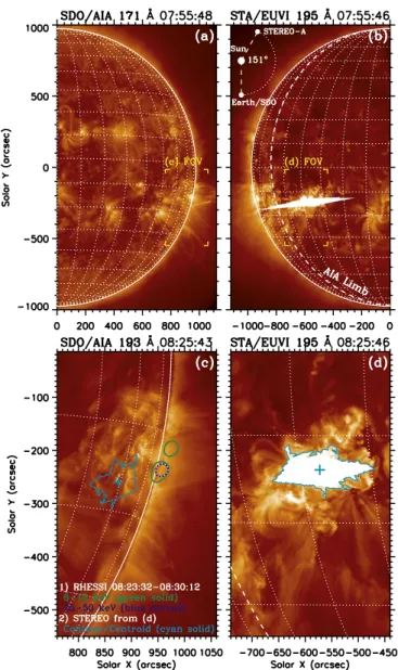
For the Jan14 flare, the Fermi-LAT photon statistics were not sufficient to provide an emission localization error circle smaller than 0°.5. However, we can still conclude that the emission detected by Fermi-LAT was consistent with the position of the Sun. In Figure 7 we show the STEREO-A and SDO images of this event at two different times. The top panels of Figure 7 present SDO 171Å (left) and STEREO-A 195Å (right) image at 07:55:46 UT and show the filament eruption, while the bottom panels show the SDO 193Å (left) and STEREO-A 195Å (right) images at 08:25:46 UT with the RHESSI 6–12 and 25–50 keV contours of this flare.
The Fermi-LAT >100 MeV emission centroid of Sep14 is located at heliocentric coordinates[−720″, 610″] with a 68% error radius of 100″. RHESSI imaging shows a 6–12 keV source located above the visible limb slightly offset from the Fermi-LAT centroid, both shown in Figure 8. If the RHESSI source is the loop top of the BTL flare, then the minimum height needed for this source to be visible from ∼40° BTL would be ∼1010cm. HXR loop-top emission from
a flare located ∼40° BTL has been detected before by RHESSI(Krucker et al. 2007). Fermi-LAT measured 17 photons with energies >1 GeV; 15 of these (including a
3.5 GeV photon with an arrival time of 11:16:01 UT) arrived during thefirst 20 minutes of Fermi-LAT detection.
3. Spectral Analysis 3.1. Gamma-Ray Spectra
We performed an unbinned likelihood analysis of the Fermi-LAT data with the gtlike program distributed with the Fermi ScienceTools.57 We selected Pass 8 Source class events from a 10° circular region centered on the Sun and within 100° from the local zenith (to reduce contamination from the Earth limb).
Wefit three models to the Fermi-LAT gamma-ray spectral data. Thefirst two, a pure power law (PL) and a power law with an exponential cutoff (PLEXP), are phenomenological func-tions that may describe bremsstrahlung emission from relativistic electrons. The third model uses templates based on a detailed study of the gamma-rays produced from the decay of pions originating from accelerated protons with an isotropic pitch angle distribution in a thick-target model(updated from Murphy et al.1987).
We rely on the likelihood ratio test and the associated test statistic TS(Mattox et al.1996) to estimate the significance of the detection. The TS is defined as twice the increment of the logarithm of the likelihood obtained byfitting the data with the source and background model components simultaneously.
Figure 6.Localization of the Oct13flare. Images near the flare peak are shown for STEREO-B 195 Å (a), SDO 193 Å (b), and an enlargement of the SDO image (c) marked by the white rectangle in(b). The green circle in (b) shows the 68% error circle for the Fermi-LAT emission centroid and the green dot in (c) represents the Fermi-LAT emission centroid position. The time range for the Fermi-LAT emission is from 07:10:00–07:35:00 UT. The green contour in (c) shows the 25–50 keV RHESSI source. The blue cross in(a) and (c) marks the centroid of the STEREO flare ribbon as seen from the STEREO and Earth/SDO perspectives, respectively. The white dashed line in(a) represents the solar limb as seen by SDO. The positions of STEREO and SDO/Earth relative to the Sun are shown in the lower-right corner of(a).
57
We used the version 10-01-00 available from the Fermi Science Support Center:http://fermi.gsfc.nasa.gov/ssc/.
Because the null hypothesis (i.e., the model without an additional source) is the same for the PL and PLEXP models, the increment of the TS(ΔTS=TSPLEXP– TSPL) is equivalent
to the corresponding difference of the maximum likelihoods computed between the two models. Note that the significance inσ can be roughly approximated as TS for two degrees of freedom.
In Table 1 we list the TSPL,ΔTS, photon index Γ for the
best-fit model (PL when ΔTS < 25 or PLEXP when ΔTS 25), and PLEXP cutoff energy. For several intervals, ΔTS>25, indicating that PLEXP provides a significantly better fit than PL. For these intervals we fit the pion-decay models to the data to determine the best proton spectral index following the same procedure described in Ajello et al.(2014). In particular, we performed a series offits with the pion-decay template models calculated for a range of proton spectral indices. We then fit the resulting profile of the log-likelihood
with a parabolic function of the proton index. The minimum gives the most likely index for the pion-decay model. Note that the TS values for the PLEXP and pion-decay fits cannot be directly compared(Wilks 1938) because they are not nested models. However, PLEXP approximates the shape of the pion-decay spectrum; thus, we expect the pion-pion-decay models to provide a similarly acceptablefit.
The main contributions to the systematic uncertainties are uncertainties in the effective area; in the energy range 100 MeV to∼100GeV, these are of the order of±5%. This uncertainty applies directly to theflux values and from our previous studies on LAT-detected solar flares(Ajello et al. 2014) we find that the systematic uncertainties on the cutoff energy and photon index are also of the order of±5%.58
3.1.1. Comparison of BTL and Disk Flare Characteristics
We compare the characteristics of the>100 MeV emission associated with the three BTLflares with three disk flares with similar GOES classifications and temporally extended emis-sions and are described in Ackermann et al.(2014) and Ajello et al. (2014). In addition to spectral parameters, we also compare the total >100 MeV emitted energies, and the total energy released by protons with energy>500 MeV needed to produce the detected gamma-ray emission, based on the templates of(updated from) Murphy et al. (1987). We present these numbers along with the date, estimated GOES class, CME speed, AR position, and Fermi-LAT detection duration in Table2. The proton indexes are very similar whereas the on-disk flares appear to have more energy; this is most likely because we observed the on-diskflares over longer timescales. Peak fluxes and the total energy released by protons with E>500 MeV for Sep14 and the impulsive phase of SOL2012-03-07 are comparable.
Figure9shows the proton index as a function of time for the Oct13 and Sep14 BTL flares. We fit a constant (red dashed line) and a first-degree polynomial (blue dashed line) to the data. In the case of the constantfit, we list the best-fit value in the upper left corner, whereas for the straight-linefit, we list the value of the slope. The temporal variation over tens of minutes is not sufficient to conclude whether a softening or hardening is present for these BTLflares. In Ajello et al. (2014) we found that for the on-diskflare SOL2012-03-07 the spectrum softened with a timescale of a few hours.
3.2. X-Ray Spectra
As described above we have HXR data from three instruments: RHESSI, Fermi-GBM, and Wind. Konus-Wind was in waiting mode during the Jan14 and Sep14flares; therefore, these events were detected in only three broad energy channels, namely ∼20–78, 78–310, and 310–1180 keV, with 2.944 s time resolution. RHESSI provides only a limited coverage of these flares. For the Oct13 flare there is some overlap with Fermi-GBM during the rise of the impulsive phase. As shown in Pesce-Rollins et al.(2015) the HXR spectra of RHESSI and Fermi-GBM agree well. Fermi-GBM was in the SAA and RHESSI was in spacecraft night during the impulsive phase of the Jan14flare and detected the flare during the decay phase in only two low-energy channels. Thus, we do
Figure 7. SDO171 and 193Å (left) and STEREO-B 195 Å (right) images near the Jan14flare peak. The white dashed line in (b) and (d) represents the solar limb as seen by SDO. The cyan contour and cross in(d) mark the STEREO flare ribbon and its centroid, respectively. Their projected view as seen in the AIA perspective is shown in(c), in which the centroid is located 20° behind the western limb. The green solid and blue dotted contours in (d) show the RHESSI 6–12 and 25–50 keV sources, respectively. The rectangular brackets in (a) and (b) mark the field of view for (c) and (d), respectively.
58
A more detailed description of the systematic uncertainties tied to the effective area of the LAT can be found here:http://fermi.gsfc.nasa.gov/ssc/
not have sufficient data for a spectral fit. For the Sep14 flare, RHESSI gives information only on the decay phase of the flares. In the following we show results from the analysis of the Fermi-GBM data for the Oct13 and Sep14 flares.
3.3. Combined Spectroscopic Studies
For both Oct13 and Sep14, we performed a combined Fermi-GBM/LAT fit using the XSPEC package (Arnaud1996). The spectral fits were done by minimizing PGSTAT, a profile likelihood statistic that takes into account Poisson error on the total count spectrum and Gaussian error on the background. In order to obtain the background-subtracted spectra of the Fermi-GBM data for Sep14, we used both Fermi-Fermi-GBM-NaI and Fermi-GBM-BGO spectra accumulated before the flare (from 10:54 UT to 10:57 UT) and after the flare (from 11:42-11:50 UT). For Oct13, because there was a minor on-disk flare whose onset time was 7:01 UT, we used the procedure described in Pesce-Rollins et al. (2015), which consists of using the background estimation tool developed in Fitzpatrick et al. (2012) with an additional 5% systematic error. For the LAT, we follow the procedure used in Ajello et al. (2014) and Pesce-Rollins et al. (2015) that consists of deriving the background spectrum directly from the model of the background used in the standard LAT likelihood analysis(first using gtlike and then gtbkg), and obtaining the response of the LAT using gtrspgen(all of these tools are available in the Fermi ScienceTools). The combined spectral energy dis-tribution(SED) derived from the Fermi-GBM and Fermi-LAT data extending from 30 keV to 10GeV for these flares is
shown in Figures 10and11, respectively, and the parameters for the spectralfit for both solar flares are listed in Table3.
The Oct13flare had a very weak signal in the BGO, and the best-fit model (M0) consisted of a single PL and the pion-decay
templates to describe the bremsstrahlung and >60 MeV emission detected by Fermi-GBM and Fermi-LAT, respec-tively. For the Sep14flare, the best-fit model (M0) consisted of
a single PL with an exponential cutoff at high energies to describe the bremsstrahlung emission, and the pion-decay templates to describe the >60 MeV emission detected by Fermi-LAT, similar to what was done for the 2010 June 12 Fermi flare(Ackermann et al. 2012). We also tested the statistical significance of an extra PL with a high-energy cutoff (model M1). To this end, we performed Monte Carlo
simulations(using XSPEC fakeit) by generating a spectrum described by the best-fit model (M0). We then re-optimized the
parameters of M0byfitting it to the simulated data. We finally
compared the improvement of PGSTAT when fitting the simulated data with the model M1. The improvement of
PGSTATfor the Oct13 and Sep14flares is ΔPGSTAT≈408 and
≈109, respectively. Despite these high values of ΔPGSTAT,
dedicated Monte Carlo simulations indicate that they corre-spond to significances of 2.5σ and 2.0σ, respectively.
We then checked whether the addition of the 2.223 MeV line (on top of the model M0) significantly improved the fit. For the
Oct13 flare, the improvement was negligible (ΔPGSTAT≈0),
while for the Sep14 the improvement was ΔPGSTAT≈25,
corresponding to a significance of 2.0σ, estimated from Monte Carlo simulations. We tested whether adding nuclear de-excitation narrow lines and continua provided an improvement
Figure 8.Localization of the Sep14flare. Images near the time of the flare peak are shown for STEREO-B 195 Å (a), SDO 193 Å (b), and an enlargement of the SDO image(c) marked by the white rectangle in (b). The yellow circle in (b) and (c) shows the 68% error circle for the Fermi-LAT emission centroid. The time range of the Fermi-LAT data is from 11:02:00–11:20:00 UT. The green contour in (b) shows the 6–12 keV RHESSI source. The blue cross in (a) marks the STEREO flare ribbon centroid, whose projected position as seen by SDO is shown in(b) and (c) with the same symbol. The white dashed line in (a) represents the solar limb as seen by SDO.
to the fit for both flares and found that it was not significant. The nuclear line and continua templates used here are based on a detailed study of the nuclear gamma-ray production from accelerated ion interactions with elements found in the solar atmosphere(Murphy et al.2009).
3.4. Radio Spectra
The radio spectra obtained at the peaks of the Oct13 and Sep14 events are shown in Figure 12. The spectrum was obtained by using the RSTN one-second resolutionfluxes. The spectra were background subtracted and the fluxes were integrated within the selected time intervals for each frequency. For each spectrum we detected the frequency where the maximum flux was observed. The spectra of the Oct13 and Sep14 flares are similar to those expected from the gyro-synchrotron (GS) mechanism, with peaks that separate the optically thin and thick parts(for GS spectrum properties see, for example, Dulk1985). The values for the microwave photon spectral index, α, for both flares are shown in Figure 12. Unfortunately, the RSTN data for the time period of the Jan14 flare are not sufficient to obtain radio spectra.
4. Solar Energetic Particles
Interpretation of the origin of SEPs is more complicated than studying photons, since they move with different velocities along curved magneticfield lines and are detected only when thefield lines are connected to the instrument. Moreover, they may be scattered by turbulence with energy-dependent mean free path. The GOES protonfluxes did not show a significant increase for the Oct13 event(which occurred behind the eastern limb). However, STEREO-B, positioned behind the limb and with better magnetic connectivity, detected an increase of SEP proton intensity starting roughly 2 hr after the detection of an electromagnetic signal from this flare. The Sep14 flare, however, which was located roughly 40° behind the eastern limb, was associated with an increase in the proton fluxes detected both by STEREO-B (which had a front view of the flare) and GOES (starting roughly 9 hr after the flare).
The Jan14flare, originating in an AR 20° behind the western limb, produced no significant increase in the proton flux at STEREO, had better magnetic connectivity to the Earth, and was associated with a very strong SEP event with neutrons detected on the ground by the South Pole neutron monitors.
The arrival timeT2(Debrunner et al.1988) at the Earth of a
particle with velocity v=βc released from the Sun at time T1,
Table 1
Fermi-LAT Spectral Analysis of the Solar Flares Considered in this Work Time Interval TSPL ΔTS
a
Photon Indexb Cutoff Energyc Fluxd Proton Index (UT) (MeV) (×10−5ph cm−2s−1) SOL2013-10-11 07:10:00–07:15:00 20 3 −2.0±0.4 L 0.9±0.1 L 07:15:00–07:18:00 487 43 −0.4±0.4 130±30 17±1 4.5±0.4 07:18:00–07:20:00 846 77 −0.1±0.4 112±21 49±2 4.3±0.2 07:20:00–07:22:00 776 76 −0.3±0.3 128±23 46±2 4.4±0.3 07:22:00–07:24:00 677 58 −0.2±0.4 153±31 29±2 3.7±0.2 07:24:00–07:26:00 345 25 −0.9±0.4 208±61 21±2 3.9±0.3 07:26:00–07:28:00 219 34 0.6±0.7 86±22 16±1 4.5±0.4 07:28:00–07:40:00 283 29 0.1±0.7 86±26 7±1 5.3±0.4 SOL2014-01-06 07:55–08:15 67 20 −2.4±0.2 L 0.6±0.1 L SOL2014-09-01 11:02:00–11:04:00 42 9 −2.5±0.3 L 11±3 L 11:04:00–11:06:00 321 41 −0.2±0.5 117±27 117±10 4.7±0.4 11:06:00–11:08:00 1070 120 −0.5±0.3 116±15 360±17 5.2±0.2 11:08:00–11:10:00 1549 126 −0.9±0.2 158±20 477±19 4.9±0.2 11:10:00–11:12:00 2549 115 −1.2±0.2 194±28 565±21 4.8±0.2 11:12:00–11:14:00 6394 157 −0.8±0.1 167±10 522±20 4.4±0.1 11:14:00–11:16:00 2430 159 −0.6±0.2 148±17 540±22 4.5±0.2 11:16:00–11:18:00 1069 32 −1.9±0.2 488±90 465±23 4.2±0.2 11:18:00–11:20:00 1047 49 −1.0±0.3 182±37 396±27 4.5±0.2 12:29:00–12:34:00 56 12 −2.2±0.2 L 3±1 L 12:34:00–12:39:00 133 3 −2.3±0.2 L 3±1 L 12:39:00–12:44:00 130 5 −2.2±0.2 L 2±1 L 12:44:00–12:49:00 97 11 −2.3±0.2 L 2±1 L 12:49:00–12:54:00 84 3 −2.4±0.2 L 2±1 L Notes. a ΔTS=TSPLEXP– TSPL. b
Photon index from the best-fit model. The PL is defined asdN EdE( ) =N E0 Gand the PLEXP as =N E expG -dN E dE E E 0 c ( ) ( )
, where Ecis the cutoff energy.
c
From thefit with the PLEXP model.
d
is ⎛ ⎝ ⎜b⎞⎠⎟= +z ´ b T T c 1 1 , 1 2 1 ( )
where ζ is the distance traveled by the SEP from the acceleration region to the Earth. Assuming scatter-free propagation for the first-arriving particles, ζ will be indepen-dent of particle energy or velocity and will be equal to the path length along a Parker spiral magneticfield line from the Sun to the Earth(usually assumed to be 1.2 au). If all the particles are accelerated at the same place and time, then the intercept of the linefitting T2to 1/β would give T1, the time at which SEPs are
released and is known as the Solar Particle Release(SPR) time. The slope of this line,ζ/c, will be of the order of 600s.
Since we do not have high energy resolution SEP data we obtain the SEP onset times using two methods depending on the energy range of the particles. For the GOES SEPs with energies <200 MeV we apply a median filter to the intensity profile and define the onset time as when the profile reached 5% of the maximum. For the higher-energy SEPs we apply a Fast Fourier Transform(FFT) filter to the intensity profile and evaluate the time when the second derivative is maximum as
Table 2
Comparison Between Behind-the-limb and On-disk Flare Quantities
Date GOESa CME Speedb AR Duration Peak Fluxc Eγ>100 MeVd Protone Ep>500 MeV
f
(UTC) Class (km s−1) Position (minutes) (10−5ph cm−2s−1) (erg) Index (erg) 2013-10-11 M4.9 1200 N21E103 30 49±2 1.5×10²³ 4.3±0.1 9.8×1024 2014-01-06 X3.5 1400 S8W110 20 0.8±0.1 4.2×10²¹ 5.3±0.4g 3.5×10²³ 2014-09-01 X2.4 2000 N14E126 113 565±14 1.4×1024 4.7±0.1 7.0×1025 On-diskflares 2011-03-07 M3.7 2125 N30W48 798 3±1 5.1×10²³ 4.7±0.2 3.6×1025 2011-06-07 M2.5 1255 S22W53 38 3±1 3.2×10²² 5.0±0.3 2.5×1024 2012-03-07Ih X5.4 2684 N16E30 45 417±13 3.9×1024 3.90±0.02 2.1×1026 2012-03-07Ei X5.4 2684 N16E30 1068 97±2 1.4×1025 4.3±0.1 9.0×1026 Notes.
aGOESclass for BTL flares is estimated based on the STEREO 195 Å flux. b
Speed is the linear speed reported by the LASCO CME catalog.
c
For photon energies>100 MeV.
d
Total energy released in>100 MeV gamma-rays integrated over the time interval when ΔTS>25.
e
Proton index in the same time interval as(d).
f
Total energy released by protons with E>500 MeV estimated over the same interval as in (d). Values may be underestimated for flares with centroids at heliocentric angles>75°.
g
TheΔTS value for this flare is 20, so the improvement over a power law is marginal.
h
Impulsive phase of theflare, Fermi-LAT detection from 00:38:52-01:23:52 UT. Note that the peak of the GOES X-ray flare occurred ∼6 minutes prior to Fermi orbital sunrise.
i
Extended phase of theflare, starting from 02:27 UT.
Figure 9. Proton index inferred from thefitting of the gamma-ray emission with the pion-decay templates as a function of time for Oct13(top panel) and Sep14(bottom panel). The red dashed lines represent a fit with a constant and the blue dashed lines a linear fit. Fit parameter values and p-values are indicated in each panel.
Figure 10.Combined Fermi-GBM/LAT count spectra (top panel) and spectral energy distribution(middle panel) for the Oct13 flare integrated between 7:10 and 7:35 UT; the lower panel shows the residuals of thefit. The models that bestfit the data are a power law that dominates the low-energy spectrum and a pion-decay model, which describes the Fermi-LAT spectrum. The neutron capture line(at 2.223 MeV, highlighted by the red vertical dashed line) is not statistically significant, and neither is an additional low-energy power law with exponential cutoff(∼2.5σ). The parameters of the fits are listed in Table3. The Astrophysical Journal, 835:219 (13pp), 2017 February 1 Ackermann et al.
the onset time. To estimate of the uncertainty on the onset time we performed a scan over a series of values for the median and FFTfilter windows and take the difference in onset times as the error.
The onset times as a function ofb1 for the GOES SEP protons associated with Jan14 are shown in Figure13. Fitting the data
to Equation (1), we estimate the SPR time to be T1=07:55±0:05 UT and the path length ζ∼1.3±0.2 au.
The value for T1is consistent with the estimated SPR time,
07:47 UT, reported by Thakur et al.(2014) but is somewhat later than the start of theflare activity at the Sun. Since Fermi was in the SAA and RHESSI was in orbital night, the most accurate time of the initiation of the flare was obtained from Konus-Wind and STEREO data. Konus-Wind detected emission in the 21–78 keV energy range starting at 07:43 UT, implying an emission time at the Sun of 07:35 UT, roughly 12 minutes prior to the SPR time. Assuming that the CME was released at this latter time, the acceleration of SEPs started when the CME was at a height of 1.5Re(vCME/1400 kms−1).
Unfortunately, the high-energy SEP data were not sufficient to estimate the SPR time for the other two BTL flares that occurred on Oct13 and Sep14.
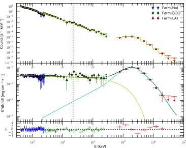
Figure 11.Combined Fermi-GBM/LAT count spectra (top panel) and SED (middle panel) for the Sep14 flare integrated between 11:02 and 11:20 UT; the lower panel shows the residuals of thefit. The best-fit models are a power law with exponential decay at high energy to describe the emission from 30 keV to ∼10 MeV and a pion-decay model to describe the Fermi-LAT spectrum. The neutron capture line(at 2.223 MeV, highlighted by the red vertical dashed line) is not statistically significant (∼2σ) and neither is an additional power law at low energy∼2σ. The fit parameters are listed in Table3.
Table 3
Best-fitting Spectral Parameters of the Fermi-LAT and Fermi-GBM Data
Parameter Value
SOL2013-10-11 Best-fit model: PL1+PION
Power-law(1) index 3.2±0.1 Proton Index 4.1±0.1
PL1+PL2×EXP+PION
Power-law(1) index 3.4±0.06 Power-law(2) index −0.9±0.3 Cutoff energy(MeV) 0.8±0.1 Proton Index 4.1±0.1
SOL2014-09-01 Best-fit model: PL1×EXP+PION
Power-law(1) index 2.06±0.01 Cutoff energy(MeV) 90±7 Proton Index 4.4±0.1
(PL1+PL2)×EXP+PION
Power-law(1) index 2.18±0.01 Power-law(2) index 1.4±0.3 Cutoff energy(MeV) 10±0.1 Proton Index 4.4±0.1 Note.Model parameters for both the Oct13 and Sep14flares. For the Oct13 flare we integrated between 7:10 and 7:35 UT, and for the Sep14 flare we integrated from 11:02 and 11:20 UT. The parameters of the best-fit model are compared with those of a more complex model with double power laws at low energy(whose improvement is not statistically significant).
Figure 12.Radio spectra during the peaks of the HXR and radio time profiles (07:09:30–07:10:20 UT) for the Oct13 flare in red and for the Sep14 flare in blue(11:09:00–11:10:00 UT). The microwave photon spectral index α, found byfitting the optically thin part of the spectra for each flare, is also shown.
Figure 13. Onset times as a function of 1/β for the GOES SEP protons associated with Jan14. The Y-axis gives the time in seconds since 2014-01-06 07:40 UT (assumed start of the flare as detected by STEREO-B) assuming scatter-free propagation for the first-arriving particles. The red dashed line represents thefit using Equation (1), giving the path length ζ=1.3±0.2 au
5. Summary and Discussion
We have presented the analysis of Fermi-LAT data from three BTL solar flares, whose location is determined by STEREO observations. We also presented analyses of data from RHESSI, Fermi-GBM, and Konus-Wind in the HXR range; SDO in EUV; RSTN in radio wavelengths; some SEP observations; GOES; and the South Pole Neutron Monitors. We found several results.
1. The HXR LCs measured by the three instruments (in overlapping energy ranges) are in good agreement with each other and with the high-frequency radio LCs. The Fermi-LAT emission, in general, commences several minutes after the HXRs, peaks at a later time, and lasts longer.
2. We are able to obtain RHESSI images in soft HXRs for flares just over the limb, indicating a loop-top emission from loops with heights above the photosphere ranging from 0.2×10¹⁰ to 2×1010 cm. SDO detected UV emission for Oct13, and possibly Jan14, but not for the Sep14 flare. The Jan14 flare was too weak to permit localization of the gamma-ray source, but localizations of the Fermi-LAT emission with Pass 8 data for the other two flares situates the centroid locations near the solar limb and about 50″ (Oct13) and 300″ (Sep14) from the RHESSI centroid.
3. The LCs(available only for the Oct13 and Sep14 flares) show good agreement between the HXR spectra measured by Fermi-GBM, RHESSI(whenever contem-poraneous data are available), and Konus-Wind below a few 100 keV. The Fermi-LAT spectra can befitted with a relatively hard PLEXP phenomenological model (possi-bly due to relativistic electron bremsstrahlung) or to a pion-decay model with proton indexes around 4. We note that production of photons of about ∼3 GeV detected here requires >15 GeV protons or >6 GeV electrons. These energies are greater than any other reported for solar particles.
4. We compare several spectral properties of >100 MeV radiation from the BTLflares with those of three on-disk flares previously analyzed. As evident from Table 2 and Figure 9, in general, these flares have similar character-istics. Similar GOES classflares have similar peak photon fluxes, surprisingly, regardless of limb occultation. The higher total gamma-ray energy of on-disk flares most likely results from their having been observed over longer timescales. Thus, the underlying acceleration and emis-sion processes are most likely similar, but the transport paths of the radiating particles(presumably protons) from the acceleration to the emission site must be different. That is, for BTL flares, protons must travel greater distances to land on the front side of the Sun to produce the detected gamma-rays.
5. Wefind that the proton index does not vary significantly during the 30 minute observation time windows for the BTL flares. This is similar to that found for the on-disk flares for the same time frames, but some on-disk flares are detected over longer time intervals (up to 20 hr) during which the proton index increases gradually. We now present our interpretation of these results with the goal of constraining the emission and acceleration mechanisms and sites.
5.1. SEP Onset Times
Since the spectral information available for the Jan14flare is limited, we cannot constrain the acceleration, transport, or radiation processes. However, thisflare is remarkable because the AR, being located beyond the western limb, provided good magnetic connection with the Earth and as a result it was associated with a very strong SEP event and increased the neutronflux in the South Pole neutron monitor. As presented in Figure13, the acceleration time at the Sun for the SEP protons is 07:55±0:05 UT, which is in agreement with the SPR time of 07:47±0:08 UT reported by Thakur et al. (2014). Unfortunately, Fermi-LAT was in the SAA at the SPR time and exited at 07:55 UT. Therefore, we can only provide an upper limit on the time of acceleration of gamma-ray-producing particles (presumably protons) at the Sun. However, Konus-Wind detected emission in the 20–78 keV band starting at 07:43 UT, implying that the electrons were accelerated at the Sun at 07:35 UT, roughly 12 minutes prior to the SPR.
Due to the location of the AR, the other twoflares were not magnetically well connected to the Earth. For the Sep14flare, the GOES protonfluxes begin to increase roughly 9 hr after the flare start time. STEREO-B observed the flare in its entirety but provides protonfluxes only in three energy bands, which is not sufficient to estimate the acceleration time at the Sun as we did for Jan14. Thus, we do not have reliable SEP data to test whether the onset times of the SEP and gamma-rays coincide; however, we can compare the height of the CME at the time of the gamma-ray onset with the CME height at SPR found for Jan14. Based on the second-orderfit of height as a function of time(from the LASCO CME online catalog), we estimated that the CME was at∼2.5Reat the onset time of the Fermi-LAT emission. We found a similar value for Oct13. These heights are significantly smaller than the predicted values reported in Thakur et al.(2014) for the CME heights at SPR as a function of source longitudes from Solar Cycle 23. To test whether these CME heights are compatible with the gamma-ray emission detected from the BTLflares, detailed simulations on particle transport in the solar magneticfield are required. This study is beyond the scope of this paper and will be addressed in a future work.
5.2. Spatial Distributions
The RHESSI images show that the 20–50 keV HXRs, due to electron bremsstrahlung, are emitted from ≈30″ (L ∼ 2 × 109 cm) and ≈50″ (L ∼ 3.5 × 109 cm) sources from the tops of loops extending to heights of ∼4×10⁹ and ∼2×1010 cm above the photosphere for the Oct13 and Sep14 flares, respectively. The column depth required for a particle of mass m and kinetic energy E(in units of mc2), or Lorentz factor
g=E+1 =(1 -b2)-1 2, to lose all its energy via Coulomb interactions is
ò
p b g = L = ´ -N r m m dE m m E 4 ln 5 10 cm , 2 e E e Coul 02 1 0 2 22 2 2 ( ) ( ) ( ) ( )where r0is the classical electron radius and lnL ~20 is the
Coulomb logarithm. From Equation(2) we find that the column depth required to stop the>50 keV electrons that produce the HXRs detected by RHESSI is ∼5×1020cm−2. Assuming a density of n<1010cm−3, the sizes of the loop-top sources imply a column depth of NLT<2 and 3.5×1019cm−2for the
two HXR sources, respectively. This means that the energy-loss time tCoul~ N2 Coul (vn) is more than 10 times longer than
the crossing time tcrossºL v=NLT (vn). These values,
together with the results reported in Chen & Petrosian (2013), suggest that the HXR emission from these two BTL flares are thin-target sources.
If these loop-top sources were to be produced in a thick target, which can come about in two ways, it would be under extreme conditions not likely to be the case here. Thefirst is in the strong diffusion limit, i.e., if the electrons are trapped because the scattering time, τsc, is smaller than the crossing
time, τcross. Note that because tCoul>tcross, the scattering cannot be due to Coulomb interactions but it could be due to turbulence. The second possibility is in the weak diffusion limit
tsc>tcross, where trapping can occur if thefield lines converge strongly. In this case we need tsc>tCoul h59(with proportion-ality constant η increasing with increasing field convergence(Petrosian 2016)). These are somewhat extreme conditions requiring either a very high density (therefore increasing the scattering, presumably turbulence) or a some-what strong field convergence and a “clean” loop with low density and low level of turbulence.
Thus, the HXR emission is most likely due to electron bremsstrahlung from a thin-target loop-top source.
Based on the positions of the Fermi-LAT >100 MeV emission centroids alone, we cannot exclude that the gamma-rays come from the loop-top source. In order to investigate this possibility, we rely on Equation (2) to find the column depth required to stop >350 MeV protons (which produce >100 MeV photons) and find NCoul(350 MeV)~1025 cm−2. This is much larger than the loop-top column depth NLT∼2–3.5×1019cm−2so that, in the absence of trapping,
we are again dealing with a thin-target loop-top source and a small energy loss compared to what would be the case for emission from a thick-target photospheric source. Conse-quently, we would need much larger energies of accelerated protons than those given in Table 2 assuming a thick-target scenario. The condition for proton trapping in the loop top(or any coronal trap region, for that matter) is also more extreme than that described above for electrons, and we would need escape times 105times longer than the crossing time. Thus, the emission detected by the Fermi-LAT is most likely due to decay of pions produced by energetic protons interacting in a thick-target photospheric source.
5.3. Spectral Distributions
As shown in Lin & Hudson (1971) and McTiernan & Petrosian(1990), in a thin-target scenario the relation between the HXR spectral index,γ, and the number index of the energy spectrum of the emitting electrons60 through bremsstrahlung processes, δ, is ⎧ ⎨ ⎩ d g g
= - 0.5 non relativistic case,
relativistic case. 3
-( )
For optically thin synchrotron radiation, the relation betweenδ and the microwave photon spectral index,α, can be described by the following relations for the relativistic (e.g., Rybicki & Lightman1979) and semirelativistic (e.g., Dulk1985) cases
d a
a
= +
+
1.1 1.36 semi relativistic case,
2.0 1 relativistic case. 4
{
-( ) We will use these relations in the following for the interpretation of the detected emission from the two brightest BTLflares reported in this work. The spectra of the two flares in the 30 keV–10 MeV energy range are somewhat different so we discuss them separately.
Oct13: As already shown in Pesce-Rollins et al.(2015), both RHESSI and Fermi-GBM detect HXR spectra for the Oct13 flare that are relatively steep (the best-fit value of the power-law photon indexγ = 3.2 ± 0.1). However, as shown in Figure10, there is a tentative indication that the spectrum may harden into a nearly flat part in the 1–10 MeV range, requiring either a similar hardening of the spectrum of the accelerated electrons, as, e.g., described in Park et al.(1997), or a contribution from de-excitation nuclear lines. We found that the inclusion of a 2.223 MeV broad neutron capture line and the nuclear de-excitation lines did not improve thefit significantly and that the best-fit model for the emission observed by Fermi-GBM is a single PL.
As described in Section5.2, the thin target is most likely, in which case following Equation (3) for the nonrelativistic case (<100 keV) the index of the electron number density δ∼2.7. The radio spectrum observed by RSTN, shown in Figure 12, indicates microwave flux of 60 solar flux units (6 × 10⁵ Jy), which peaks at frequencyν∼5 GHz and declines as n-awith the index α∼2 above this frequency. Based on the relations described in Equation(4), we find that the required power-law index for the number density of electrons to be δ∼5 or δ∼3.5 in the relativistic or semirelativistic regime, respectively.
These values are steeper than the indexδ∼2.7 required in the nonrelativistic HXR range, indicating a steepening of the electron spectrum above 1 MeV. We therefore conclude that the GBM flux in the energy range 300 keV–10 MeV is probably not due to the accelerated electrons and no extra component is expected.
Sep14: The best-fit model for the combined HXR Fermi-GBM gamma-ray emission from the Sep14flare is a single PL with an exponential decay with photon index 2.06±0.01 and a cutoff energy of 90±7 MeV. This is an extremely hard spectrum for a solarflare and if it is produced by a thin-target electron bremsstrahlung model as described above, it would require an electron number spectrum with indexδ∼1.5 in the nonrelativistic range steepening to an index δ∼2 in the relativistic range. However, as noted above, inclusion of the 2.223 MeV line improves thefit slightly, indicating a possible contribution from nuclear de-excitation lines so the steepening of the electron spectrum could be larger.
The radio spectrum of thisflare, shown in Figure12, is also harder. The emission detected by the San Vito station has an index α∼1 above 1 GHz. Again assuming optically thin synchrotron emission would require semirelativistic electrons with electron power-law index δ∼2.5, indicating a slightly larger steepening at high energies. If the magnetic field is lower, which could be the case because of the larger loop, the steepening would be even larger (δ ∼ 3). Thus, for the Sep14 59
According to Malyshkin & Kulsrud(2001), h ~ln(B0 BL), the log of the
ratio of magneticfield strengths at the middle and ends of a magnetic bottle.
60
This should not be confused with the electronflux,F E( )=vN E ,( ) index, which in the nonrelativistic limit is dlnF E( ) dlnE=g-1.0, used commonly. In the relativistic regime these indexes are equal and as stated in Equation(3) δ=γ.
flare a power-law spectrum, steepening at higher energies, is required to explain the HXR and microwave observations from the loop-top region. This, plus a pion-decay component, provides an acceptable fit to theFermi data from 30 keV to several GeV.
5.4. Acceleration Site and Mechanism
The above interpretation of the HXR and MWs indicates that the electrons responsible for these emissions are most likely accelerated in the reconnection region above the loop-top source either by turbulence(Petrosian 2012) or in merging islands manifested in the particle-in-cell simulations(Drake & Swisdak2012). The electrons are trapped in the loop-top region long enough (longer than the crossing time of a fraction of second) to produce detectable bremsstrahlung and synchrotron radiation, but most of their energy is lost in thick-target footpoints hidden from near-Earth instruments because of high optical depths(Pesce-Rollins et al. 2015). This scenario can also explain the HXR emission from a BTL flare reported by Krucker et al.(2007). The steepening of the electron spectrum in the semirelativistic regime is due to a decrease in the acceleration rate and not to transport or energy-loss effects.
If the Fermi-LAT emission is from a thick-target photo-spheric site, then this emission site is located on the visible part of the disk. It cannot come from the occulted AR. The fact that accelerated protons reach the on-disk emission site provides strong evidence that the acceleration site is the CME environment, as suggested by Cliver et al. (1993) and Pesce-Rollins et al.(2015). They would diffuse across a wide range of magneticfields, some connected to the AR behind the limb and some to the visible side of the Sun. These ions will most likely come from the downstream region of the CME shock while SEPs escape the upstream region. This can account for the differences in their spectral and temporal characteristics. It is then possible that the discrepancy between the spectral characteristics in 1–10 MeV for the GBM and radio observa-tions can be explained by lower-energy 1–100 MeV protons or electrons precipitating to the visible disk side from the downstream region and producing the 1–10 MeV nuclear de-excitation line or bremsstrahlung emission below the chromo-sphere. These and other possibilities, for example, the production of Fermi-LAT emission by relativistic electrons either in the CME shock, in reconnection regions on current sheets behind the CME, or trapped in a large loop with strong convergence, will be discussed in future papers.
The Fermi-LAT Collaboration acknowledges support from a number of agencies and institutes for both development and the operation of the LAT as well as scientific data analysis. These
include NASA and DOE in the United States, CEA/Irfu and IN2P3/CNRS in France, ASI and INFN in Italy, MEXT, KEK, and JAXA in Japan, and the K.A.Wallenberg Foundation, the Swedish Research Council, and the National Space Board in Sweden. Additional support from INAF in Italy and CNES in France for science analysis during the operations phase is also gratefully acknowledged. W.L. was supported by NASA HGI grant NNX16AF78G and LWS grant NNX14AJ49G. V.P., W.L., and F.R.d.C. are supported by NASA grants NNX14AG03G, NNX13AF79G, and NNX12AO70G. V.P. and L.K. are grateful for RFBR grant 15-02-03717. We thank Nariaka Nitta and Meng Jin for friutful discussions on SEPs and magnetic connectivity.
References
Ackermann, M., Ajello, M., Albert, A., et al. 2014,ApJ,787, 15
Ackermann, M., Ajello, M., Allafort, A., et al. 2012,ApJ,745, 144
Ajello, M. A. A., Allafort, A., Baldini, L., et al. 2014,ApJ,789, 20
Aptekar, R. L., Frederiks, D. D., Golenetskii, S. V., et al. 1995,SSRv,71, 265
Arnaud, K. A. 1996, in ASP Conf. Ser. 101, Astronomical Data Analysis Software and Systems V, ed. G. H. Jacoby & J. Barnes(San Francisco, CA: ASP),17
Atwood, W. B., Abdo, A. A., Ackermann, M., et al. 2009,ApJ,697, 1071
Barat, C., Trottet, G., Vilmer, N., et al. 1994,ApJL,425, L109
Chen, Q., & Petrosian, V. 2013,ApJ,777, 33
Cliver, E. W., Kahler, S. W., & Vestrand, W. T. 1993, ICRC,3, 91
Debrunner, H., Flückiger, E., Grädel, H., Lockwood, J. A., & McGuire, R. E. 1988,JGRA,93, 7206
Drake, J. F., & Swisdak, M. 2012, in APS April Meeting Abstracts, 3-D Particle-in-cell Simulations of the Sawtooth Crash,(Altana, GA), K1.022 Dulk, G. A. 1985,ARA&A,23, 169
Fitzpatrick, G., McBreen, S., Connaughton, V., & Briggs, M. 2012, Proc. SPIE,8443, 3
Hurford, G. J., Schmahl, E. J., Schwartz, R. A., et al. 2002,SoPh,210, 61
Krucker, S., White, S. M., & Lin, R. P. 2007,ApJL,669, L49
Lin, R. P., & Hudson, H. S. 1971,SoPh,17, 412
Malyshkin, L., & Kulsrud, R. 2001,ApJ,549, 402
Mattox, J. R., Bertsch, D. L., Chiang, J., et al. 1996,ApJ,461, 396
McTiernan, J. M., & Petrosian, V. 1990,ApJ,359, 541
Meegan, C., Lichti, G., Bhat, P. N., et al. 2009,ApJ,702, 791
Murphy, R. J., Dermer, C. D., & Ramaty, R. 1987,ApJS,63, 721
Murphy, R. J., Kozlovsky, B., Kiener, J., & Share, G. H. 2009,ApJS,183, 142
Nakajima, H., Nishio, M., Enome, S., et al. 1994,IEEEP,82, 705
Nitta, N. V., Aschwanden, M. J., Boerner, P. F., et al. 2013,SoPh,288, 241
Park, B. T., Petrosian, V., & Schwartz, R. A. 1997,ApJ,489, 358
Pesce-Rollins, M., Omodei, N., Petrosian, V., et al. 2015,ApJL,805, L15
Petrosian, V. 2012,SSRv,173, 535
Petrosian, V. 2016,ApJ,830, 28
Rybicki, G. B., & Lightman, A. P. 1979, Radiative processes in astrophysics (New York: Wiley-Interscience),393
Saldanha, R., Krucker, S., & Lin, R. P. 2008,ApJ,673, 1169
Thakur, N., Gopalswamy, N., Xie, H., et al. 2014,ApJL,790, L13
Thompson, W. T., & Wei, K. 2010,SoPh,261, 215
Vestrand, W. T., & Forrest, D. J. 1993,ApJL,409, L69
Vilmer, N., Trottet, G., Barat, C., et al. 1999, A&A,342, 575
Wilks, S. S. 1938,Ann. Math. Stat.,9, 60