A new instrument for space plasma exploration: The current density coil

HAL Id: hal-00405925

https://hal.archives-ouvertes.fr/hal-00405925

Submitted on 11 Jan 2021

HAL is a multi-disciplinary open access

archive for the deposit and dissemination of

sci-entific research documents, whether they are

pub-lished or not. The documents may come from

teaching and research institutions in France or

abroad, or from public or private research centers.

L’archive ouverte pluridisciplinaire HAL, est

destinée au dépôt et à la diffusion de documents

scientifiques de niveau recherche, publiés ou non,

émanant des établissements d’enseignement et de

recherche français ou étrangers, des laboratoires

publics ou privés.

A new instrument for space plasma exploration: The

current density coil

A. Meyer, L. Rezeau, F. Mottez, H. de Feraudy, A. Roux

To cite this version:

A. Meyer, L. Rezeau, F. Mottez, H. de Feraudy, A. Roux. A new instrument for space plasma

exploration: The current density coil. Journal of Geophysical Research, American Geophysical Union,

2001, 106, pp.12999-13006. �10.1029/2000JA900131�. �hal-00405925�

JOURNAL OF GEOPHYSICAL RESEARCH, VOL. 106, NO. A7, PAGES 12,999-13,006, JULY 1, 2001

A new instrument for space plasma exploration:

The current density coil

A. Meyer, L. Rezeau,

F. Mottez, H. de Feraudy,

and A. Roux

Centre d'Etude des Environnements Terrestre et Planttaires, Universit6 de Versailles St Quentin en Yvelines, v61izy, France

Abstract. This paper presents

an instrument

aimed at measuring

current

densities

in space

plasmas:

a current

density

coil. Such

an instrument

already

exists

for the estimation

of currents

in

the laboratory.

A special

design

has been

developed

and tested

for use on board

spacecraft.

The

characteristics

of the instrument

are explained

in details and many tests

performed

on the ground

are presented.

It is shown

that the current

density

coil is sensitive

enough

to measure

ionospheric

currents.

1. Introduction

A new instrument is proposed to measure current densities in space plasmas: a current density coil (CDC). On existing spacecraft such a measurement has never been included, although attempts to develop a current sens• have already been done. A Danish team is developing a coil based •n Faraday rotation of laser light in an optical fiber [Primdahl et at 1•9.•86];

to our knowledge

its sensitivity

is around

10 I.

tAm -2. To obtain

To date, the current density can be derived from particle instruments or magnetometers (DC or AC), but a direct measurement would greatly improve the understanding of the physics. Our aim is to fly this instrument on future spacecraft that will explore regions where the currents are expected to play an important role, mainly in the auroral region, but also in the solar corona. A first set of tests of the coil is presented in this paper, including laboratory tests and numerical simulations.

The paper is organized as follows: After a presentation of the principle on which the instrument works and a short description

of its technical realization, the testing equipment and the tests

procedures are presented in detail. Then the measurement

capabilities of the CDC are described, showing that it is suited for space plasma investigations and that the obtained sensitivity is accurate for the space plasma measurements that should be performed in the future. Of course, since no direct measurement of the current density has ever been performed before, no rigorous comparison can be made; we can only use estimates

deduced from other measurements.

Section 5 of the paper is dedicated to an analysis of the limits of the instrument. We study the magnetic field perturbations by

the instrument itself, the constraints due to the finite size of the

coil, the effects of the potential of the blanket which covers the coil on the electrons that carry the current, and the effect of secondary electrons emitted by the blanket. The study of the effects of variations of the coil potential is important since, in space, it has been shown that the potential of a spacecraft can Copyright 2001 by the American Geophysical Union.

Paper number 2000JA900131.

0148-0227/01/2000JA900131 $09.00

vary quite a lot and reach values as high as 100 V [Wahlund et

al, 1999].

2. Description of the Current Density Coils

2.1 Physical Principle on Which the Coil Works

The CDC consists of a large number of wire turns wounded on a toms made of magnetic material. As in an electric transformer,

an AC current passing through the surface of the torus induces

an AC magnetic field in the torus and therefore produces an emf

in the winding. The induced emf is, e=laOlarNSR/2 d<jn>/dt,

where N is the number of wire tums, S is the meridian cross

section of the loop, R is the main radius of the torus, and jn is the

current density in the direction normal to the loop plane. A

consequence of this formula is that the coil is not sensitive to

static currents; in fact, as it will be put on board a rocket or a

spacecraft, the relative motion of the vehicle with respect to the

plasma will provide temporal variations and make the current

measurable if its spatial scale is not too large. The principle of

the coil is not very different from that of the search coil

magnetometers that have been flown on many spacecraft to

measure AC magnetic fields [S-300 Experimenters; 1979,

Cornilleau-Wehrlin et al, 1997]; therefore one might imagine

that the CDC is sensitive also to magnetic fields. As will be

shown in section 3, a suitable design of the winding gives a strict cancellation of the magnetic flux, thus making the coil sensitive only to AC currents.

As can be seen from the formula given above, a CDC measures the projection of the current density on the direction

parallel to its axis. Therefore, to measure the vectorial current

density a set of three perpendicular coils is necessary.

2.2 Technical Realization

All the figures given in the paper correspond to technical characteristics of the same prototype coil (SN03, diameter 30 cm), although several coils have been tested, with sizes from 8 to 30 cm. The core of the coil is made of a high permeability material (relative permeability gr = 250,000) to reach a high sensitivity. The toms shape of the core is obtained by winding a continuous thin sheet of material in a circular shape until a square section of- 1 cm side is obtained (Figure l a.) Two flat washers of the same material are then placed on the top and the bottom of the core to isolate it from external magnetic fields.

13,000 MEYER ET AL.: TECHNIQUES

(b)

Figure 1. Schematic drawing of the coil illustrating (a) lhe winding of the magnetic material in the core (vertical

lines in the cross section), and (b) the successive layers of the wire that make the primary winding.

This toms is then wrapped with two windings (as for search coil magnetometers). The main winding has a very large number of tums (20,000), and it is wound alternately forward and backward to cancel the magnetic flux in the whole winding (Figure lb). Actually, each layer is equivalent to one turn of radius R that would be sensitive to DC or AC magnetic fields; by winding an even number of layers, symmetrically, this sensitivity is cancelled [Meyer, 1995]. As shown in Figure 2, the transfer function of this primary winding is a resonance curve with a maximum around 155 Hz, a low-frequency slope of 6 dB/octave (corresponding to the inductive behavior of the coil) and secondary resonances above 4 kHz. To obtain a flat transfer function in a wide frequency range, a secondary winding is used

to introduce flux feedback. To smooth the unavoidable

secondary resonances, a low-pass filter is added. A high-pass filter is also added, which modifies the low frequency slope to

12 dB/octave; its role is to lower the possible effects of parasitic very low-frequency signals, such as a possible DC drift of the

preamplifier or a signal at the spin frequency. Its cutoff

frequency is adjusted to the spin frequency of the spacecraft.

The resulting transfer function is shown on Figure 2: it is flat

over almost three decades. This frequency range can be adjusted

to the characteristics of the spacecraft on which the coil is

80 60 > 40 • 20 • 0 -20 -40

, IIIIII IIIIII • IIIII IIIII f I IIIIII IIIIII IIIIII '•111 IIIII ! I IIIIII IIIIII II!111 Ilgl, IIIII IIIIIII IIIIII IIIIII IIII1• IIIII IIIIIII IIIIII /• IIIIII IIII1• IIIII IIIIIII IIIIII r •, IIIIII IIIII • IIIII IIIitll IIIIII \ III111 IIIII •11111 IIIIIII IIIIII \ IIIIII IIIII NIIII II II111 IIIIII • •1111 IIIII I•111

IIIIII .' I III1• IIIII II1•1

I IIIII/ IIIIII \ IIIII IIIII I IIIIII II]1,I1 IIIIII •. •1111 IIIII

I IIIIII •1111 IIIIII ß •11 IIIII

IIIII/ IIIIII IIIIII IIIII '•111

I I Ik•l' IIIIII IIIIII IIIII I• I.•"1111 IIIIII IIIIII IIIII IIIII

/,4111111

IIIIII

IIIIII

IIIII

IIIII

ß I IIIIII IIIIII IIIIII IIIII IIIII

/ I IIIIII IIIIII IIIIII IIIII IIIII

IIIIIII IIIIII IIIIII IIIII IIIII IIIIIII IIIIII IIIII IIIII

I I I I

0,1 1 10 100 1000 10000 100000

Frequency (Hz)

Figure 2. Transfer functions of a 30-cm CDC (model SN03).

The lowest curve is the response curve of the main winding of

the coil alone. The highest one is the final transfer function, when feedback, preamplifier, and filters have been added.

flown: the low-frequency, cutoff is adjusted to the spin

frequency, and the high frequency cutoff depends on the scientific objectives and the regions that will be encountered.

The coil is finally wrapped in a conducting blanket in order to

provide a good uniformity of the potential around the probe to

minimize the perturbations of the local plasma. In the tests

described here the blanket is made of aluminum.

3. Means used to test the instrument

The preliminary tests have been performed using an AC current produced in a wire going through the coil. These tests

confirm that the principle of the instrument is valid, and they

give a calibration of its response, output volts for 1 A current in the wire. They also show that the behavior of the CDC is linear: the response does not depend on the amplitude of the current (provided that the current remains lower than values around 1 A, which is many orders of magnitude higher than the values expected in space). However, as the instrument is dedicated to measurements of currents in space plasmas, these test conditions are oversimplified. To bring complementary information about the workings of the instrument in space conditions, we have

used two different means: a test in a plasma chamber and

numerical simulations. 3.1. Plasma Chamber

We used the Jonas plasma chamber of Department

Environnement Spatial) at Office National d'Etudes et de Recherche A6rospatiales (ONERA) in Toulouse (France). It is a

3-m long stainless steel cylinder in which a cryogenic pumping

lowers

the pressure

to 10

-6 Pa. The Earth magnetic

field is

beam.

The plasma

is an argon

plasma,

with a density

of 105

cm

-3

The current measured by the coil has to be checked against other measurements to be validated. Figure 3 shows a schematic view of the experimental setup. The electron beam goes first

through

the CDC and then into an 8-cm

2 Faraday

cage.

A

MEYER ET AL.: TECHNIQUES 13,001 fluorescent disc

Faraday

o

,X

primary

winding

K

7

e- gun

½

blanket

/

Q)

Figure

3. Layout

of the instruments

in the plasma

chamber.

The CDC is represented

by a cut-away

sketch,

showing

the

toms

of magnetic

material,

the

primary

winding,

and

the

conducting

blanket.

I• is the

current

given

by

the

electron

gun,

I2 is the

current

captured

by the

Faraday

cage,

I3 is the

current

captured

by the

fluorescent

disk,

and

I4 is the current

captured

by the aluminum

blanket

of the CDC.

The output

of the CDC is the voltage

of the

preamplifier

which

is connected

to the

primary

winding

of the

CDC (Vc).

covering the CDC, as well as the current given by the electron gun. Thus a complete check of the current balance can be made.

3.2. Numerical Simulation

Because the current carried by the electron beam cannot be

varied much below 50 gA, the tests performed in the plasma

chamber do not give access to the sensitivity of the CDC. That is

why numerical simulations have complemented them. These

numerical tests also allow separate tests of various effects that

influence the behavior of the coil but cannot be distinguished in the plasma chamber experiments.

The simulation box is a 40 cm side cube filled with electrons

(we do not consider the behavior of ions, considered as a

neutralizing background). These electrons are initialized with

random positions, and a Maxwell-Boltzmann velocity

distribution, characterized by a uniform average density, a

parallel bulk velocity, and an isotropic temperature. Because of

the electron bulk velocity, this distribution carries a current. The

electrons are moving in external (not self-consistent) constant

magnetic and electric fields. These fields consist of a uniform

ambient magnetic field (parallel to the initial current), plus a

perturbation generated by the high permeability material (the

core of the loop), and an electric field caused by a potential drop

between the coil and its environment (this field is the solution of

the Laplace equation in vacuum; it does not take into account

the ambient plasma).

The CDC is placed in the middle of this box: It is a toroidal

loop with a square cross section, similar to the real one. The

comparison is made between the ambient ideal current density

determined by the initial conditions of the plasma and the current density flowing through the coil, obtained by counting

the electrons that cross the section defined by the inner part of

the loop. The discrepancy gives an indication of the error made

when using the CDC. In the simulation, unlike in real tests,

several effects can be switched off to understand their specific

role: (1) the perturbing magnetic field due to the magnetic core

of the coil and (2) the capture of the electrons which hit the coil.

If effect 2 is switched off, the coil becomes transparent to electron motion. Finally, the electric potential of the coil can be

set to three different values: 0, +10 V, and-100 V.

3.3 Comparison

of the Different

Methods

of Measuring

the

Current

In real life, in space, the current structure, whatever it is (tube,

sheet, etc,..), extends over distances much larger than the size of

the coil. Although no direct current measurements have ever

been performed, this assumption seems quite reasonable. Previous estimates made by particle or magnetic field

experiments indicate that scales as low as 100 m at an altitude of

400 km can be expected [Forget et al., 1991]. Some authors

suggest

that 100 m could be the smallest

scale

[Staciewicz

and

Potemra, 1998] which can be related to the fact that the inertial

length of the electrons at this altitude is around 100 m and that it

is the smallest physically significant scale. Observations of the

thickness of auroral arcs made from the ground give the same

order of magnitude [Borovsky, 1993]. Therefore, in any case, the

CDC will pass through current structures much larger than its

own diameter and will "catch" a small section of the current and

give a measure of the current density times its section.

In the numerical simulation the situation is similar except for

one difference: There is only an electron beam present in the

simulation box, and its charge is compensated by a stationary

ion background, and no space charge field is taken into account.

In the plasma chamber experiment, however the relative

dimensions of the coil and the current are reversed: the electron

beam covers only ~ 0.1% of the section of the coil. To explore

the whole surface and especially to study the edge effects, the

coil is translated in from of the electron beam.

4. Measurement Capabilities

4.1. Preliminary Tests in the Plasma Chamber Without

Plasma

With an electron beam carrying 50 BA, a numerical simulation shows that the current density is measured with a precision of 0.5%. With the real coil, we have to compare the obtained response in the chamber to a reference response. Calibrated with a current produced in a wire, the obtained reference transfer function at 55 Hz (in the flat part of the

function)

is 4640

V A 'l, that

is 73.3

dBV A 'l, when

the potential

13,002 MEYER ET AL.' TECHNIQUES

t•l iii• coil

cross

section

• ... . ... ? ... •. ... • ...

•

80

...

: ...

•.

...

•

...

t.

•

...

-2ffi - 1 • - 1 ffi -• 0 • 1 ffi 1 • 2ffi

x(mm)

Fibre 4. Response of the CDC as a function of the position of

the incidem electron beam (model SN03). •e size of the coil is

superimposed (d•k shaded squares). The light shaded regions

have the size of the beam.

of the coil is fixed at 0 V. In the plasma chamber the current is

measured with the Faraday cage (I2); we obtain I2 = 30 gA for

the 55-Hz part of the signal. This is consistent with the results

expected for the first harmonic frequency of a 55-Hz square

signal of amplitude switching from 0 to 50 gA. The current

through the fluorescent disk is stable around 0.2 gA and

therefore always negligible compared to the measured current.

The current through the aluminum blanket of the coil is equal to

0 except when the beam hits the coil. The coil is moved

perpendicular to the electron beam, and its response is plotted in

Figure 4, where the size of the coil is shown for comparison.

When

the beam

passes

in the central

region

of the coil (between

and 73.69 dBV/A, with an average

of 73.4 dBV A -1, which

ß represents an accuracy of less than 1%. When the beam hits the

coil, the measurement is disturbed because the current through

the aluminum shield reaches 15 gA. The asymmetry in the

response near the two edges of the coil is likely to be due to a

slight curvature of the beam (due to the magnetic field residue).

This is not comparable to the situation in space, where electrons

will continuously hit the whole surface of the coil; the shield is

designed with one strip over each of the four sides of the toms to

ensure a symmetry of the currents with respect to the axis of the

coil and therefore a balance of the currents in the shield. 4.2. Tests in the Presence of a Plasma

First of all, the CDC will be used in plasmas and therefore has

to be tested in the plasma chamber filled with plasma. In that

case, with the same current density as before and the potential of

the coil fixed to 0 V, the transfer

function

in the center

of the

coil is 73.3 dBV A -I, which is the nominal result. It is

interesting to note that the edge effects are less important when

the coil is embedded in a plasma: Considering the case where the beam is only 5 mm from the coil (if it is closer the current flows through the shield), the departure from the central measurement is 8.6% without plasma and only 3.2% with plasma. This improvement is likely to be due to the screening of the coil by the plasma, but it cannot be tested properly since the Debye length (= 8 mm) is of the same order as the beam. 4.3. Comparison of the Measurement Capabilities With the Known Values of Currents in Space Plasma

It must be noted that the current carried by the electron beam

in the plasma chamber (50 gA) corresponds to high values of the

current

density:

around

700 gA m

-2 if one assumes

that

the coil

is embedded in the current. In the auroral region the estimates of

the current are deduced from the magnetic measurements, and

the maximum values of the currents are expected to be around

300 gAm

'2 at the subkilometer

scale

[Berthelier

et al., 1991;

able to measure current densities significantly lower than those

tested in the plasma chamber. In the numerical simulation it is

not difficult to decrease the current and to show that the coil can

measure

much

smaller

currents:

a 1 gA m

'2 current

is measured

The sensitivity of the real coil can be tested in the laboratory,

in a magnetic environment that is cleaner than in a large plasma

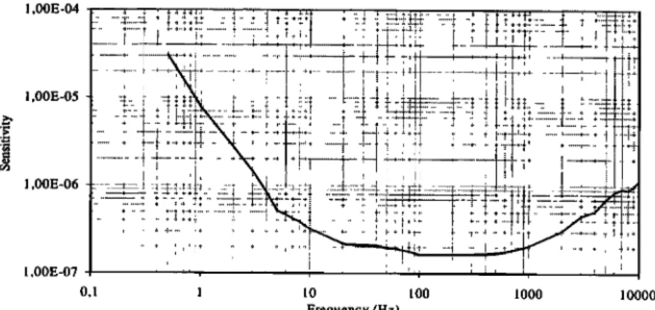
1,00E-05 1,00E-06 1,00E-07 1,00E-08 0,1 1 10 100 1000 10000 Frequency (Hz)

MEYER ET AL.: TECHNIQUES 13,003

chamber. The result obtained under these conditions is plotted in

Figure

5 and it can be compared

to the estimates

of currents

in

space.

if a relative velocity

of the spacecraft

and a current

structure of 1 km s '1 is assumed, a 100-m structure is crossed in

0.1 s and appears

as a 10-Hz signal.

For a current

density

of

200 gA m

'2 [Forget

et al., 1991]

and an analysis

with a 50%

bandwidth,

the coil needs

a 100 gA m

'2 Hz

'1/2

sensitivity

to be

values in that frequency range. Of course, the figures given here

depend on the velocity of the spacecraft

and on the

characteristics of the analysis and, hence the real sensitivity of

the coil might be slightly different. Nevertheless, it clearly

evidences that the instrument has the capability of studying

ionospheric currents. This curve also shows that structures

smaller than 100 m will also be resolved by the instrument

(corresponding

to higher frequencies),

thus allowing the

exploration

of a scale domain which so far has not been

explored.

5. Exploration of the limits of the instrument

5.1. Magnetic Perturbations Due to the Coil Material

The magnetic

material,

which

is the core of the CDC, creates

its own magnetic

moment,

which modifies

the field lines of the

nearby

external

magnetic

field. Of course,

with a real coil this

effect cannot be avoided. In the numerical simulations it can be

removed, since the measurements are made by counting the

particles

going through

the coil and not by measuring

the

induced

voltage.

One can expect

that the modification

of the

field lines will be more important if the external field lines are

far from normal to the coil plane. This effect is tested in

Figure

6, where

a current

of 1 gA m

'2

is flowing

through

the

coil

at different angles. When the angle between the current and the

magnetic

field is small, there is no difference

between

the two

aj/j (%) o

0 o 30 ø

I I I I I I

60 ø 90 ø

angle between the coil normal and the current direction

Figure 6. Error on the measurement of the current deduced

from numerical simulations. Diamonds correspond to the case

where the coil is transparent and there is no perturbing magnetic

field, pluses correspond to the case where the coil is transparent

and the magnetic field of the magnetic core is present, and dots

correspond to the most realistic case where the coil is thick and

the field is perturbed.

cases, with or without the perturbing magnetic field. When the

angle is large (80ø), the part of the current that is measured is

small, and the error on the measurement reaches 2.5%. As will be shown in section 5.2, when the coil is in a set of three coils,

this error plays a minor role since it modifies a very small

component only. In the other case, when only one coil is used,

this error is more important since it cannot be corrected as the

direction of the current is unknown. 5.2. Geometrical Effects

The finite size of the CDC introduces some unavoidable

limitations. First, as already mentioned, a given coil measures only the component of the current density that is normal to its surface, but as the angle with the normal increases, the error on

the measurement also increases. The finite size of the section of

the toms induces a loss of the particles that hit the inner side of the sensor, giving rise to a dead angle (assuming that the particles are captured and that no secondary emission occurs). For a 30-cm coil this angle is equal to 87 ø. For angles smaller

than this limit but still far from the normal of the loop, the

thickness of the coil induces an error on the estimate of the

surface "seen" by the current. This surface is smaller than the

expected

value

of •R2cosot

and has to be used

to deduce

the

can be corrected. A first estimate of the direction of the current

can be calculated; then, knowing its direction relative to one coil, the error on the corresponding surface can be corrected,

and a refined estimate of the direction can be deduced. As soon

as the current density direction is close to the normal of one of the three coils, the precision of the estimate will be excellent since the maximum error will be on very small components. The

worst situation would be when the current is as far as possible

from all the nortnals, that is around 55 ø, but then the error is less

than 1% and can be corrected.

These orders of magnitude are given for a 30-cm-diameter coil. Clearly, they increase if the• coil is smaller, because it is not possible to reduce the section of the coil in proportion to the

radius of the toms, for obvious technical reasons. However,

even in that case, the geometrical errors can be corrected. Changing the size of the coil has a consequence on its sensitivity. The sensitivity shown here (Figure 5) is that of a 30- cm coil with 20,000 wire turns. It can be compared to the sensitivity of a 15 cm coil with 16,300 wire turns (Figure 7); there is a loss of ~ 1 decade in sensitivity when the dimension is reduced by a factor of 2. When the use of the coil fixes its size (for instance a large coil cannot be flown on a rocket), the sensitivity can be improved by increasing the number of wire tums. A new 15-cm coil is being built, with 40,000 wire tums; its sensitivity is expected to reach a value equal to twice the

sensitivity of the 30 cm coil. Therefore, although it will be less

sensitive than a 30-cm coil, it will be much better than the

previous 15-cm coil.

5.3. Influence of the Electrostatic Potential of the Coil

All the tests that have been discussed in the previous sections

were performed with a grounded conducting blanket. With the

13,004 MEYER ET AL.' TECHNIQUES 1,00E-04 1,00E-05 1,00E-06 1,00E-07

"i

...

'"'

...

Figure

7. Sensitivity

(in A m

'2

Hz

'1/2)

of a 15-cm

coil

with

16,300

wire

turns.

since there is no ground and the ambient plasma influences the

potential of the instruments. Therefore tests have been

performed in the plasma chamber together with numerical

simulations with different potentials of the coil, including the

floating potential.

In the chamber, introducing a power supply in the branch where I4 is measured (see Figure 3) can modify the voltage of the coil aluminum blanket. The plasma potential is measured

during the experiments by a Langmuir probe; its value is around

0.6 V. When the potential of the blanket is left floating, it

reaches a value, around -0.6 V, which is a bit less than the

plasma potential; i.e., the coil behaves like a Langmuir probe.

Figure 8 shows the response of the CDC for different values of

the voltage of the coil blanket, with and without plasma in the

chamber. The main conclusion deduced from these tests is that

the reference response is obtained only when the potential of the

coil is kept near 0 V. When it moves away from this value, the response varies considerably. Therefore, to obtain precise

measurements in space, the voltage of the coil should be kept at

the spacecraft potential. Another interesting conclusion of this

study is about the edge effects. When the coil is tested in a

100,00 90,00

8o,0o

70,00

Figure 8. Response of the CDC in the plasma chamber as a

function of the voltage of the conducting blanket of the coil,

with plasma in the chamber (open squares) or without (solid diamonds). The thin line represents the nominal response (model

SN03).

plasma, there are less edge effects: The beam can pass closer to

the coil without being affected by it. This result, already evidenced at 0 V, is also valid at other voltages.

All these tests in the plasma chamber have been performed

with the same 3-keV electron beam. Of course, the influence of

the voltage of the coil on the beam is strongly related to the

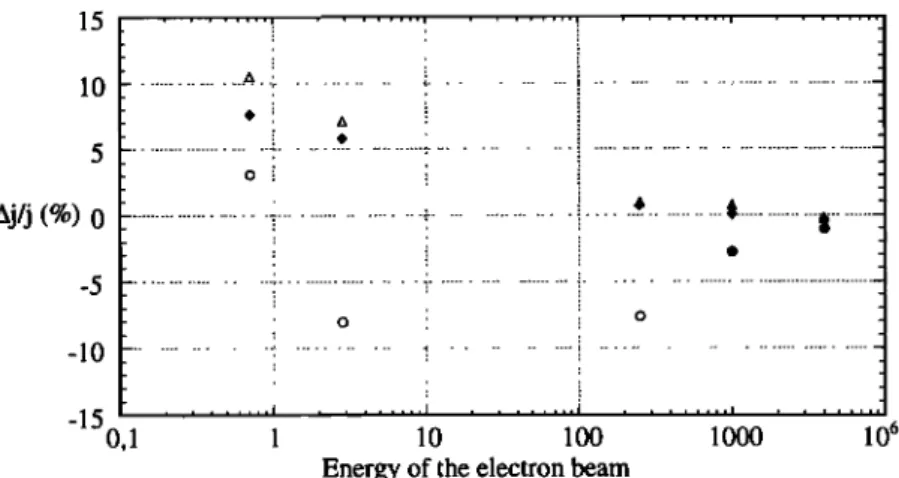
energy of the particles and to their charge. For a current carried by ions the above results should be reversed. The relative effects of the voltage of the coil and the energy of the electrons have been tested in numerical simulations. The results are presented in Figure 9, which shows that the error on the estimate of the current density increases when the energy of the beam

decreases. They also show that for low voltages the error

becomes large only for very low energies. On the other hand, for a-100-V voltage the error is higher than 5% as soon as the energy of the beam is less than a few 100 eV. These

observations are consistent with an electrostatic interaction between the beam and the coil. This means that with the real coil

in the plasma chamber the physical situation is more complicated, since the variations are not consistent with the simple electrostatic interaction. This difference is very likely due to the existence of secondary electrons emitted by the coil

itself, since in the numerical simulation this effect is not

included. Taking this effect into account, the results in Figure 8 become more clear: For a positive voltage the secondary electrons are recaptured after a short flight, and for a negative

potential the electrons are repelled from the coil and perturb the

estimate of the current. For a very negative voltage they are

strongly repelled from the coil and hence do not disturb any

longer the response of the coil; it goes very close to the nominal

one.

5.4. Perturbation

of the Measurement

by Secondary

Electrons and Photoelectrons.

As evidenced by the results shown in section 5.3, the emission

of secondary

electrons

is an important

problem

to consider

in

order to understand the behavior of the coil in all situations. A

similar problem in space, which has not been tested on the

ground,

is the emission

of photoelectrons.

The secondary-

electron

emission

yield has been

studied

for many

elements

and

compounds:

All show

the same

kind of response,

an increasing

emission

as a function

of the energy

of the incident

electrons

to

a maximum

yield and then

a decrease

[Scholtz

et al., 1996].

This

maximum

yield and the corresponding

incident

energy

then

characterize

a given

element.

For aluminum

the maximum

yield

MEYER ET AL.: TECHNIQUES 13,005 10 ... '• ... o

Aj/j

(%) 0 ...

!

...

* ...

$

...

ooo

Figure 9. Error on the measurement of the current deduced from numerical simulations as a function of the energy of the electron beam. The diamonds correspond to a grounded coil, the triangles correspond to a +10-V voltage, and the dots correspond to a-100 V voltage. The symbols are solid when the energy of the beam is higher than the voltage of the coil, and they are open when it is of the same order of magnitude or lower.

is around 1 and is obtained for 300-eV electrons; for 3-keV

electrons the yield goes down to 0.6 [Garrett, 1980].

An estimate of the number of secondary electrons that are emitted by the coil blanket can be made, taking into account the

geometry of the instrument and the known dependency of the

yield as a function of the incidence angle [Vaughan, 1989]. The

coil is covered by four strips of aluminum, one on each side of

the toms. It is most likely that the electrons produced by the outside, top side, and bottom side will not disturb the current measurement to any large extent. The main perturbation will come from the inner side. As this surface is a cylinder, the incidence angle depends on the point of incidence. By

performing integration on the entire surface, we obtain a 7%

effective yield for the coil. This value corresponds to a normal incidence of the current with respect to the coil, as it was in the

plasma chamber experiment. If we study the secondary emission

as a function of the angle between the current and the normal to the coil, we find that it is stable for angles smaller than 45 ø,

while for larger angles it increases to 50% for an angle of 80 ø .

Therefore this emission becomes a large source of error in the measurements for very large incidence angles. The error behaves in a similar way to the geometrical effect studied above; that is, if them is a set of three coils on board the spacecraft, it is a minor problem.

One can think of reducing

the effect of the secondary

electrons by choosing the best material for the cover. A comparative study of many elements [Whetten, 1962] shows that carbon has the smallest efficiency, 0.45, obtained for a 500-eV

energy when it is in soot form. A similar study for

photoemission of amorphous materials [Grard, 1973] shows that

graphite is the material that produces the smallest number of

photoelectrons. Therefore we have decided to change the

conducting blanket of our coils and replace aluminum with carbon. Preliminary tests show that the voltage of the blanket (if it is left floating) reaches the plasma potential with a much better accuracy, which should minimize the effects of secondary

electrons.

6. Conclusion

The tests which have been presented here show that the CDC

is a new instrument that is capable of improving our knowledge

of space plasma properties. First of all, it is sensitive enough to

measure the current densities that are expected in the auroral

region, as far as we know. It will also make possible the

exploration of smaller scales than the scales that can be studied using magnetometers, that is, scales that have never been explored before. The sensitivity of the coil is higher when the coil is larger; therefore the size chosen for a given spacecraft has to be a compromise between sensitivity and bulk, although small coils can be improved by increasing the number of winding

tums.

Clearly, the number of CDCs on board the spacecraft is also very important. A set of three coils will always give a good estimate of the direction and the intensity of the current density. On the other hand, a single coil will give only an estimate of the

projection of the current density with an error which might be

very large if the angle of the current direction and the coil normal is large.

The tests performed on the coil show that its response is more reliable when its potential is maintained close to 0 V, which in the case of the plasma chamber was close to the plasma potential. This indicates that in a space experiment the potential of the coil should be kept at the spacecraft potential. When the voltage of the coil departs from the ground potential, the effects of secondary electrons or photoelectrons become more important. This problem is still under study, and some improvements can be included in future models, such as a

carbon blanket instead of an aluminum one for instance.

A set of three CDC is going to be flown in December 2001 on

a rocket launched in the cusp region. A full set of plasma instruments will be on board: particle measurements and DC and

AC magnetic field measurements. This will allow a detailed

comparison

of the current

estimates

obtained

by these

three

different means. Particle instruments can give a direct estimate of the current density, but they suffer from limitation in time resolution (due to the time needed to sample all directions and energies) and from the thresholds in energy. On the other hand,

magnetometers have a high time resolution but give only an

indirect estimate of currents since the relation between currents

and field is differential. Owing to these limitations, the results

from these two instruments will allow one to check some

properties of the currents, but will not be redundant with the

13,006

MEYER ET AL.: TECHNIQUES

Acknowledgments.

The tests in the plasma chamber have been performed with financial

support of the French space agency, CNES, and of Universit6 de Versailles-Saint-Quentin en Yvelines. The authors wish to thank Franqois Lefeuvre and Vladimir Krasnosel'skikh for fruitful discussions, and Bernard Poirier, Dominique Alison, and the ONERA team for their

technical support. The computations have been supported by the CNRS

and made on a Cray 98 at IDRIS (Orsay, France)

Michel Blanc thanks the referees for their assistance in evaluating this

paper.

References

Berthelier, A., J.C. Cerisier, J.J. Berthelier, and L. Rezeau, Low

frequency magnetic turbulence in the high-latitude topside

ionosphere: low-frequency waves or field-aligned currents, J. Atmos.

Terr. Phys., 53(3/4), 333-341, 1991.

Borovsky, J. E., Auroral arc thickness as predicted by various theories,

J. Geophys. Res., 98, 6101-6138, 1993.

Comilleau-Wehrlin, N., et al., The CLUSTER spatio-temporal analysis

of field fluctuations (STAFF) experiment, Space Sci. Rev., 79(1-2),

107-136, 1997.

Forget, B., J.-C. Cerisier, A. Berthelier, and J.-J. Berthelier, Ionospheric

closure of small-sacle Birkeland currents, J. Geophys. Res., 96, 1843-

1847, 1991.

Garrett, H. B., Spacecraft charging: a review, Space Systems and their

interactions with earth • space environment, Progress in astronautics

and aeronautics, vol. 71, edited by H. B. Garrett and C. P. Pike, published byAmerican Institue of Aeronautics and Astronautics, New

York, 1980.

Grard, R. J. L., Properties of the satellite photoelectrons sheath derived

from photoemission laboratory measurements, J. Geophys. Research,

78, 2885-29060, 1973.

Krasnosel'skikh, V.V., A.M. Natanzon, A.E. Reznikov, A. Y. Schyokotov, S.I. Klimov, A.E. Kruglyi, and L.Woolliscrofi, Current

measurements in space plasmas and the problem of separating between spatial and temporal variations in the field of a plane

electromagnetic wave, Adv. Space Res., 11, (9), 37-40, 1991.

Meyer, A., Boucle de courant h contre r6action de champ, note technique, Centre d'Etude des Environ. Terr. et Plan6t.,V61izy,

France, 1995.

Primdahl, F., P. Hoeg, C. J. Nielsen, and J. E. Schroder, A new method

for measuring space plasma current densities by the Faraday rotation of laser light in optical monomode fibers, DRI $ci. Rep. 4-86, 1986. Reulet, R., L. Levy, and D. Sarrail, Etude du comportement d'une

boucle de courant en pr6sence d'un plasma ionosph6rique, Assistance technique simulation spatiale, Rapp. ONERA RF/470900/470901,

1998.

S-300 Experimenters, Measurements of electric and magnetic wave fields and of cold plasma parameters on-board GEO$ 1. Preliminary

results, Planet. Space Sci., 27, 317-339, 1979.

$choltz, J. J., D. Dijkkamp, and R. W. A. Schmitz, Secondary electron

emission properties, Philips J. Res., 50, 375-389, 1996.

Staciewicz, K., and T. Potemra, Multiscale current structures observed

by Freja, J. Geophys. Res., 103, 4315-4325, 1998.

Vaughan, J. R. M., A new formula for secondary emission yield, IEEE

Trans. Electron Devices, 36, 1963-1967, 1989.

Wahlund, J. E., L. J. Wedin, T. Carrozi, A. I. Eriksson, L. Anderson,

and H. Laasko, Analysis of Freja charging events, IRF $ci. Rep. 253,

1999.,

Whetten, N. R., Secondary electron emission, Methods of Experimental Physics, vol. 4, Academic, San Diego, Calif., 1962.

H. de Feraudy, A. Meyer, F. Mottez, L. Rezeau, and A. Roux, CETP/

UVSQ, 10-12 avenue de l'Europe, V61izy, France. (rezeau•,cetp.ipsl.t¾) (Received May 31, 2000; revised September 5, 2000, ,