HAL Id: hal-00298080
https://hal.archives-ouvertes.fr/hal-00298080
Submitted on 10 Jul 2007
HAL is a multi-disciplinary open access
archive for the deposit and dissemination of
sci-entific research documents, whether they are
pub-lished or not. The documents may come from
teaching and research institutions in France or
abroad, or from public or private research centers.
L’archive ouverte pluridisciplinaire HAL, est
destinée au dépôt et à la diffusion de documents
scientifiques de niveau recherche, publiés ou non,
émanant des établissements d’enseignement et de
recherche français ou étrangers, des laboratoires
publics ou privés.
the glacial-interglacial record of Southern Ocean silica
cycling
A. Ridgwell
To cite this version:
A. Ridgwell. Application of sediment core modelling to interpreting the glacial-interglacial record of
Southern Ocean silica cycling. Climate of the Past, European Geosciences Union (EGU), 2007, 3 (3),
pp.387-396. �hal-00298080�
Clim. Past, 3, 387–396, 2007 www.clim-past.net/3/387/2007/
© Author(s) 2007. This work is licensed under a Creative Commons License.
Climate
of the Past
Application of sediment core modelling to interpreting the
glacial-interglacial record of Southern Ocean silica cycling
A. Ridgwell
School of Geographical Sciences, University of Bristol, Bristol, UK
Received: 4 December 2006 – Published in Clim. Past Discuss.: 20 December 2006 Revised: 26 June 2007 – Accepted: 4 July 2007 – Published: 10 July 2007
Abstract. Sediments from the Southern Ocean reveal a meridional divide in biogeochemical cycling response to the glacial-interglacial cycles of the late Neogene. South of the present-day position of the Antarctic Polar Front in the At-lantic sector of the Southern Ocean, biogenic opal is gener-ally much more abundant in sediments during interglacials compared to glacials. To the north, an anti-phased relation-ship is observed, with maximum opal abundance instead oc-curring during glacials. This antagonistic response of sedi-mentary properties provides an important model validation target for testing hypotheses of glacial-interglacial change against, particularly for understanding the causes of the con-current variability in atmospheric CO2. Here, I illustrate a time-dependent modelling approach to helping understand climates of the past by means of the mechanistic simulation of marine sediment core records. I find that a close match be-tween model-predicted and observed down-core changes in sedimentary opal content can be achieved when changes in seasonal sea-ice extent are imposed, whereas the predicted sedimentary response to iron fertilization on its own is not consistent with sedimentary observations. The results of this sediment record model-data comparison supports previous inferences that the changing cryosphere is the primary driver of the striking features exhibited by the paleoceanographic record of this region.
1 Introduction
The Southern Ocean can be through of as the Achilles Heel of the modern global carbon cycle, with changes in: biolog-ical productivity (Martin, 1990; Watson et al., 2000), ver-tical mixing and stratification (Francois et al., 1997; Tog-gweiler, 1999; Toggweiler et al., 2006), and sea-ice cover
Correspondence to: A. Ridgwell
(Stephens and Keeling, 2000) all suspected of playing a key role in modifying atmospheric CO2 on glacial-interglacial time scales. Changes in the surface ocean environment of this region will be manifested in interlinked properties of sedi-mentary material deposited to the ocean floor, thus recording the mechanism(s) at work in controlling the observed CO2 variability. However, the paleoceanographic evidence from the sediments of this region has not proved possible to inter-pret unambiguously (Anderson et al., 2002; Elderfield and Rickaby, 2000; Sigman and Boyle, 2000). The difficulty faced in quantitative reconstruction of the surface environ-ment directly from sedienviron-mentary properties is a consequence of the different nonlinear processes that interact to determine a particular sediment state (i.e., the measured proxy value).
A promising modelling methodology is available to ad-dress this model-data divide – working forwards from an ex-plicit description of the biogeochemical processes involved towards the observations. By recording the properties of biogenic material preserved in deep-sea sediments within an ocean-sediment carbon cycle model, sediment core records can be generated (Heinze, 2001; Ridgwell, 20071). This relatively data-friendly model output can then be contrasted rather directly with the observed sediment record. Here I il-lustrate the potential of this approach by evaluating the con-sequences of two possible drivers of glacial-interglacial en-vironmental change in the Southern Ocean against measured changes in sedimentary opal content.
2 Modelling methodology
In this study, I use the ocean-sediment carbon cycle model of Ridgwell (2001). This is based on a zonally-averaged representation of ocean circulation, shown schematically in Fig. 1. To better resolve the effect on sediment composition 1Ridgwell, A.: Interpreting transient CCD changes by marine
sediment core modeling, Paleoceanography, submitted, 2007.
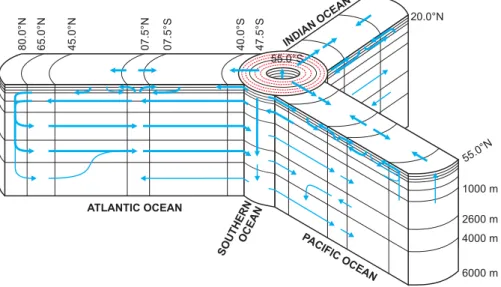
ATLANTIC OCEAN SOUTHERN OCEAN INDIAN OCEAN PACIFIC OCEAN 80.0°N 65.0°N 45.0°N 07.5°N 07.5°S 40.0°S 47.5°S 20.0°N 55.0°N 6000 m 4000 m 2600 m 1000 m 55.0°S
Fig. 1. Structure of the zonally-averaged model of marine biogeochemical cycling. Ocean circulation is delineated by blue arrows. The
sub-division of the 2 southern-most zonal boxes in the underlying ocean circulation model into 6 boxes in the version employed here is highlighted in red.
of changes in sea-ice cover in the Southern Ocean, the two 7.5◦zones south of 55◦S in the parent model are sub-divided into a total of six sub-zones of width 2.5◦ as described in Ridgwell (2001). Each of these sub-zones is assumed to be characterized by the same vertical velocity as its parent zone with meridional velocities obtained by linear interpo-lation between 55◦S and 62.5◦S and extrapolation south of 62.5◦S.
Overall, ocean-atmosphere biogeochemistry is similar to that used in previous work on the atmospheric CO2 implica-tions of glacial-interglacial (Watson et al., 2000) and anthro-pogenic (Ridgwell et al., 2002) changes in aeolian iron sup-ply to the ocean. Tracers advected in the ocean component include total dissolved inorganic carbon (DIC), dissolved oxygen (O2), alkalinity, temperature, and salinity. Of these, CO2and O2are exchanged with a “well-mixed” atmosphere across the air-sea interface. The stable isotopes of carbon (12C and13C) are treated separately, with all major fractiona-tion processes between them taken into account. Three nutri-ents potentially limiting to biological activity in the ocean are considered; phosphate (PO4), silicic acid (H4SiO4), and total dissolved iron (Fe). Nutrients, together with DIC and ALK, are taken out of solution in the sunlit surface ocean layer (eu-photic zone) through biological action, and exported as par-ticulate organic matter, CaCO3, and opal to deeper layers. As this particulate material settles through the water column, it is subject to remineralization processes, resulting in the release of dissolved constituent species to the ocean. Significant ex-port of nutrients and carbon in the form of dissolved organic matter is not considered in this particular model.
Biogenic and detrital material reaching the ocean floor may undergo diagenetic alteration, with a further release of
dissolved species to the ocean, or it may be buried in ac-cumulating sediments. To accomplish this, the ocean is ev-erywhere underlain by a series of discrete sediment modules handling ocean-sediment interactions, in which the preserva-tion of biogenic CaCO3and opal reaching the sediment sur-face is explicitly predicted. Loss of material through burial in the sediments is balanced over the long-term by prescribed inputs to the ocean representing continental weathering and geothermal processes (in the case of DIC, ALK, and H4SiO4) as well as aeolian input at the surface (for Fe). For full de-scription and evaluation of atmosphere-ocean-sediment car-bon cycling in the model, readers are referred to Ridgwell (2001) and Ridgwell et al. (2002).
The configuration of deep-sea sediments is similar in na-ture to that of earlier box modelling work (Munhoven and Francois, 1996; Walker and Opdyke, 1995). Sediments are considered at 15 discrete water depths, spanning the depth of the ocean interior from 6000 m up to base of the eu-photic zone (100 m), for a total of 315 separate sedimen-tary modules (i.e., 15 for each of the 21 ocean grid points). Each sediment module comprises a single, 5 cm thick homo-geneous surface layer, underlain by a series of 1 cm thick sub-layers, illustrated in Fig. 2. The surface layer repre-sents the upper zone of the sediment where solid compo-sition is near homogeneous with depth and where the pri-mary diagenetic processes take place. Excess solid mate-rial is exported out of this surface layer (i.e., buried) and stored in a stack of sedimentary sub-layers lying immedi-ately below. The presence of the stack enables the progres-sive erosion of material during times of net dissolution at the sediment surface to be accounted for, a process which is critical to the millennial-scale buffering of atmospheric CO2
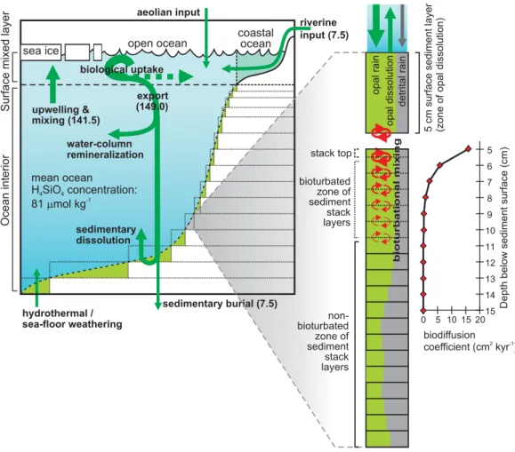
A. Ridgwell: Modelling glacial-interglacial changes in sedimentary opal 389 Surface mixed layer Ocean interior mixing (141.5) water-column remineralization hydrothermal / sea-floor weathering sedimentary burial (7.5) riverine input (7.5) upwelling & coastal ocean open ocean opal rain opal dissolution detrital rain bioturbated zone of sediment stack layers stack top non-bioturbated zone of sediment stack layers 5 cm surface sediment layer (zone of opal dissolution) biodiffusion coefficient (cm kyr )2 -1 5 6 7 8 9 10 Depth below sediment surface (cm) 15 10 5 0 bioturbational mixing 12 11 14 13 15 20 sea ice sedimentary dissolution aeolian input biological uptake export (149.0) mean ocean H SiO concentration: 81 mol kg 4 4 m -1
Fig. 2. Schematic of global biogeochemical cycling in the model and structure of the sediment modules. The initial state of the marine
silica cycling is indicated, with fluxes (of Si as either silicic acid or biogenic opal) in units of Tmol Si yr−1. The positioning of the 15
sediment modules are indicated by dotted boxes with their structure shown to the right of the figure alongside the prescribed biodiffusion mixing profile. Each comprises a 5 cm thick surface layer in which diagenesis is assumed to take place, underlain by a stack of (1 cm thick) storage or sediment compositional “memory” layers. The preservation of calcium carbonate (CaCO3)in the sediments is also calculated (see, Ridgwell, 2001; Ridgwell and Hargreaves, 2007) but not shown in this schematic.
(Ridgwell and Hargreaves, 2007). It also provides a means of simulating how changes in the solid and isotopic compo-sition of the sediments in response to global environmen-tal change (glacial-interglacial cycles in this example) are recorded in the marine record.
In addition to the advective transfer of solids between the surface layer and the stack arising from net sedimentary ac-cumulation/erosion, a transfer of material is prescribed be-tween sub-layers representing the vertical mixing of solids by the action of benthic animals – bioturbation. The effect of bioturbation is modeled here as a quasi-diffusive process (Pope et al., 1996), with the mixing rate between pairs of layers in the sediment stack determined by a biodiffusion coefficient which decreases with an e-folding depth of 1 cm and has a maximum mixing rate at the top of the stack of 16 cm2kyr−1adapted from Peng et al. (1979) (and see Ridg-well, 2001). Mixing also occurs between the surface layer
and upper-most sediment stack layer. The prescribed biodif-fusion profile is shown in Fig. 2.
One advantage that modelled sediment records have over the data is that the precise age of material deposited to the sediment surface is known. A numerical tracer of the time of deposition is used to tag material reaching the sediment surface, allowing a mean age for each sediment sub-layer to be tracked (Ridgwell, 2001). In this way, an internal age-scale is generated, alleviating the need for the tuning of a δ18O stratigraphy to an orbital template (e.g., Bassinot et al., 1994).
The model is run over approximately four glacial-interglacial cycles (400 kyr) following an initial 150 kyr spup. Ideally, ocean biogeochemical processes would be in-formed by a suite of surface environmental boundary con-ditions (such as dust flux and sea-ice extent) generated in-ternally within an integrated Earth system model. Instead,
Age (kyr BP) 0 100 200 2.2 1.1 6 5.5 4.2 7.5 7.3 7.1 RC13-254 0 40 80 RC13-259 25 50 75 100 wt% opal wt% opal 0 40 80 simulated core @ 51.25°S 25 50 simulated core @ 56.25°S 75 wt% opal wt% opal 250 150 50 1.0 2.0 3.0 0.0
mean dust supply over 47.5°S to 70°S (g m yr )-2 -1 V22-108 wt% opal simulated core @ 43.75°S wt% opal 200 240 280 Atmospheric CO (ppm) 2 0 10 20 0 10 20 100 Antarctic Polar Front
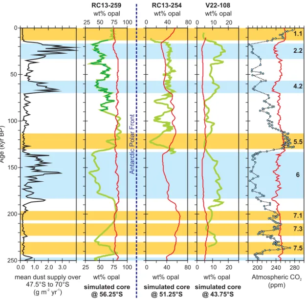
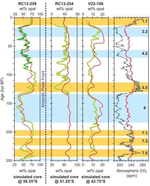
Fig. 3. Influence of glacial-interglacial variability in aeolian Fe supply on the sedimentary opal record of the Southern Ocean. Warm
(interglacial) and cold (peak glacial) marine isotope stages (Bassinot et al., 1994) are highlighted in orange and blue, respectively. Left-hand panel: dust flux forcing (Watson et al., 2000) applied to the region 47.5◦S to 70◦S in the model. The middle 3 panels show observed (thick
green line, top axis scale) and model-predicted (red line, bottom axis scale) down-core variability in wt% opal content for sediment cores lying either side of the APF. Observed data is based on cores: RC13-259 (53.9◦, 04.9◦W), RC13-254 (48.6◦S, 05.6◦W), and V22-108
(43.2◦S, 03.2◦W), all taken from the Atlantic Sector of the Southern Ocean (Charles et al., 1991; Mortlock et al., 1991). Core RC13-259
exhibits an anomalous pattern through Stages 3 and 4 compared to other cores south of the APF in this area (Mortlock et al., 1991), a result of a hiatus occurring around this level (Anderson, R. F., personal communication). Data from the nearby core RC11-77 (L. H. Burckle, personal communication) is therefore spliced into the interval ∼12–90 kyr BP, marked in dark green. Each synthetic core is recovered from a grid point having approximately the same frontal coordinate (Chase et al., 2003), that is, a similar relative latitude to the position of the APF in the model (taken to be 55◦S) as the real cores (where the observed APF in the Atlantic sector of the Southern Ocean is ∼50◦S (Mortlock et
al., 1991)). The simulated sediment core wt% opal signal is plotted using an internal age stratigraphy (Ridgwell 2001). Far right-hand panel shows observed (black dotted line with blue circles marking the data points) (Petit et al., 1999) and model simulated (red line) atmospheric CO2.
because this particular model lacks an interactive climate component, a time history of surface environmental bound-ary conditions is generated by the transformation of paired paleoclimatic reconstructions (made at discrete time slices)
by a suitable continuous proxy signal – e.g., see Ridgwell (2001), Watson et al. (2000), or K¨ohler and Fischer (2006).
A. Ridgwell: Modelling glacial-interglacial changes in sedimentary opal 391 3 Testing hypotheses for G-I change using synthetic
sed-iment cores
Records of biogenic opal content in deep-sea sediments from the Atlantic sectors of the Southern Ocean reveal a pro-nounced meridional asymmetry (Charles et al., 1991; Mort-lock et al., 1991; Kumar et al., 1995; Anderson et al., 1998), with glacial-interglacial changes in composition of sites ly-ing approximately either side of the position of the present-day Antarctic Polar Front (APF) being opposite in sign (e.g., see Fig. 3). To the south, interglacial-age sediments are char-acterized by higher opal contents than that which occurs dur-ing glacial periods, while to the north, it is glacial sediments that are the more opal-rich. These changes are paralleled by indicators of Si utilization (De La Rocha et al., 1999), sug-gesting that the antagonistic sedimentary response in wt% opal primarily reflects a change in the surface ocean environ-ment and biogenic opal export. I now force the model with time varying glacial-interglacial changes in surface ocean boundary conditions and analyse the resulting signals con-tained in the simulated sediment core records to help inter-pret these observations.
3.1 Aeolian iron supply
Enhanced aeolian iron supply to the glacial Southern Ocean has been hypothesized to drive a stronger biological pump and lower the concentration of CO2in the atmosphere (Mar-tin, 1990). Although considerable uncertainties remain re-garding the operation of the iron cycle in this region (Ridg-well and Watson, 2002), results from ocean carbon cycle models go some way to supporting the iron hypothesis and suggest that changes in dust supply may have been respon-sible for anywhere between 5 and 45 ppm of the observed glacial-interglacial variability in atmospheric CO2(Archer et al., 2000; Bopp et al., 2003; Watson et al., 2000). Changes in iron availability at the ocean surface may be potentially in-tertwined with glacial-interglacial changes in opal accumu-lation in the underlying sediments as follows. The physio-logical effects of enhanced Fe availability on diatom cellu-lar composition and more efficient utilization of silicic acid (Watson et al., 2000) has been hypothesized to lead to “leak-age” (increased transport) of H4SiO4to lower latitudes dur-ing glacials (Brzezinski et al., 2002; Matsumoto et al., 2002). This might potentially help explain the reduction in opal ac-cumulation observed to the south of the APF (Sigman and Boyle, 2000), but increased to the North. To test whether aeolian iron supply plays a fundamental controlling role in the export of opal from the surface ocean of this region, the model is forced with a varying dust flux signal to the South-ern Ocean (47.5–70.0◦S) following Watson et al. (2000). The forcing function together with the resulting predicted changes in the last 250 thousand years of sediment accumu-lation in the Southern Ocean are shown in Fig. 3.
South of the APF, a change in aeolian iron supply has lit-tle effect on sedimentary opal content, while to the north, model sediments are strongly anti-phased with the data. Al-though organic carbon export in the model is enhanced by ∼100% south of the APF as a result of increased Fe availabil-ity during the last glacial, the model-parameterized effect of Fe availability on Si utilization efficiency by diatoms (mani-fested in the Si:C export ratio (Ridgwell, 2001)) restricts the increase in opal export to just ∼34%. The increased opal rain to the sediments is partly offset by a 14% draw-down of the glacial silicic acid (H4SiO4)inventory compared to the subsequent (present) interglacial, which enhances opal dis-solution rates. There is also an increase in the dust dilution of opal during the glacial which further decouples the change in wt% opal recorded in the sediments from the opal rain rate. The net result is that there is relatively little imprint of higher productivity on the sedimentary opal record at this location.
To the north, a slight reduction in advected Si supply cou-pled with greater Si utilization efficiency during glacial times combine to produce a substantial decrease in opal accumula-tion, contrary to the data. While different assumptions re-garding the dependence of Si:C export ratios on Fe availabil-ity could conceivably improve the simulation, it is unlikely that a simultaneous match could be achieved to the data both north and south of the APF.
Of the total ∼90 ppm amplitude of glacial-interglacial CO2variabilty, 27 ppm is explained by this mechanism. The model predicted phasing between decreases in dust forcing and initial increases in CO2is consistent with observations as previously found (Watson et al., 2000) despite arguments that an apparent lag in response of up to ∼5 kyr exists (Broecker and Henderson, 1998). This can be understood in terms of a highly non-linear response of the carbon cycle to dust (Ridg-well and Watson, 2002; Gaspari et al., 2006). Thus, although the effects of dust are consistent with the timing of the ob-served intra-glacial variability in atmospheric CO2, the sedi-mentary (opal) record is not consistent with the iron hypoth-esis as a sole driver of biogeochemical changes in the South-ern Ocean between glacials and interglacials.
3.2 Sea-ice extent
Reconstructions of the cryosphere at the time of the Last Glacial Maximum (LGM) indicate that seasonal sea-ice cover was much more extensive than today in the Southern Ocean. In addition to being suggested as exerting a strong control on atmospheric CO2 (Stephens and Keeling, 2000), this surface environmental change is also central to expla-nations for the observed paleoceanographic features of this region (Anderson et al., 2002; Charles et al., 1991; Crosta and Shemesh, 2002; Sigman and Boyle, 2000). However, the highly non-linear nature of sedimentary opal preserva-tion (Archer et al., 2000; Ridgwell et al., 2002) and the un-obvious coupling relationship between opal export and sea-ice cover (Chase et al., 2003) point to the need for analysis
2.2 1.1 6 5.5 4.2 7.5 7.3 7.1 RC13-254 0 40 80 RC13-259 25 50 75 100 wt% opal wt% opal 20 60 100 simulated core @ 51.25°S 25 50 simulated core @ 56.25°S 75 wt% opal wt% opal 0 10 20 simulated core @ 43.75°S wt% opal 200 240 280 Atmospheric CO (ppm) 2 Age (kyr BP) 0 100 200 250 150 50 0.5 0.0
fractional sea ice cover south of model APF
(55°S to 70°S) 1.0 V22-108 wt% opal 0 10 20 100 Antarctic Polar Front
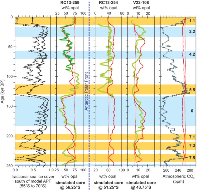
Fig. 4. The influence of glacial-interglacial variability in the seasonal limits of sea-ice extent on sedimentary opal content. Left-hand panel:
change in maximum/wintertime (continuous line) and minimum/summertime (dotted line) fractional sea-ice cover applied to the model Southern Ocean (shown averaged over all model grid points lying south of the APF). Other panels as per Fig. 3. Note the shift in the wt% opal scale for the simulated core at 51.25◦S relative to observations (RC13-254). The effect on wt% opal variability and atmospheric CO2
of applying an alternative forcing assumption of CLIMAP winter-time sea-ice extent but with fixed modern summer-time extent is shown as a red dotted line.
within a numerical model to quantify whether changes in sea-ice extent could give rise to the observed features of the opal record.
As an illustration of how the cryosphere can modulate the sedimentary record, seasonal sea-ice limits are now modi-fied in the model with present-day wintertime and summer-time fractional sea-ice coverage of each model grid point taken from CLIMAP (CLIMAP, 1976) and interpolated at intermediate months according to monthly insolation. The maximum and minimum seasonal limits are then varied over the course of approximately four glacial-interglacial cycles, taking information regarding the timing and rate of change
from the Vostok temperature record (Petit et al., 1999) and taking the absolute amplitude of the envelope from the dif-ference between present-day and LGM CLIMAP reconstruc-tions (Fig. 4). This assumes that a first-order correspondence exists between sea-ice cover and Antarctic air temperature, an assumption supported by coupled climate model results (Gildor amd Ghil, 2002).
In contrast to the large decrease in atmospheric CO2 (>45 ppm) reported in a box model of the ocean carbon cycle (Stephens and Keeling, 2000), a relatively muted re-sponse (∼7 ppm) is found here to increased glacial sea-ice cover in the Southern Ocean (Fig. 4). This disparity may
A. Ridgwell: Modelling glacial-interglacial changes in sedimentary opal 393 2.2 1.1 6 5.5 4.2 7.5 7.3 7.1 RC13-254 0 40 80 RC13-259 25 50 75 100 wt% opal wt% opal 20 60 100 simulated core @ 51.25°S 25 50 simulated core @ 56.25°S 75 wt% opal wt% opal 0 10 20 simulated core @ 43.75°S wt% opal 200 240 280 Atmospheric CO (ppm) 2 Age (kyr BP) 0 100 200 250 150 50 V22-108 wt% opal 0 10 20 100 Antarctic Polar Front
Fig. 5. The effect of both dust and seasonal sea-ice limits combined. Sediment core record and atmospheric CO2panels as per Fig. 3.
be a consequence of the lack of any explicit representation of equatorial up-welling zones (regions of intense CO2 out-gassing in the modern ocean (Takahashi et al., 1997)) in more highly idealized box models which can result in the Southern Ocean becoming the dominant source of CO2 to the (mod-ern) atmosphere (Stephens and Keeling, 2000). While the sea-ice forcing has little apparent impact on the global car-bon cycle it does drive a marked change in sediment compo-sition as shown in Fig. 4. Some of the primary features of the opal record are now well reproduced, particularly the transi-tions into and out of cold glacial stages (e.g., 2.2, 4.2, 6) and immediately following glacial inception in RC13-259. Cru-cially, the characteristic antagonistic variability either side of the APF is captured. This is a simple consequence of in-creased seasonal sea-ice cover south of the APF restricting biogenic export during glacials, with previously utilized
nu-trients advected northwards and fuelling greater (mainly di-atom) export to the north (Anderson et al., 2002).
Recent reconstructions of the past state of the cryosphere have suggested that the minimum (summer-time) limit may have been little changed (e.g., Crosta et al., 1998; Gersonde et al., 2005). I have therefore tested the sensitivity of model predictions to assumptions about LGM sea-ice cover in an additional experiment in which the CLIMAP reconstruction is again used to inform the winter-time extent in the model, but the summer-time extent is now fixed at modern. The re-sulting recorded variability in wt% opal exhibits the same anti-phased response either side of the APF (Fig. 4). How-ever, the amplitude of the variability is now substantially re-duced.
3.3 Changes in iron fertilization and sea-ice extent com-bined
Simultaneously applying both dust and sea-ice extent forc-ings leads to a further improvement in down-core opal vari-ability, shown in Fig. 5. Of the total ∼90 ppm amplitude of glacial-interglacial CO2 variabilty, 35 ppm is explained by these two mechanisms together.
4 Discussion
The information contained in the model sediments is de-termined by processes and environments representing large spatial means. In contrast, cores recovered from the deep sea may be influenced by local processes such as up-welling (Bertrand et al., 1996) and sediment redistribution by bot-tom currents (Bareille et al., 1994). Moreover, in order to maximize the temporal resolution of core data, drilling lo-cations are often chosen where such local processes result in enhanced sedimentation rates. Close model-data corre-spondence in the absolute values of opal content is thus not expected a priori.
Despite these caveats, the match for core RC13-259 (Fig. 5) is surprisingly good, lending confidence to the plau-sibility of the model assumptions. It should be noted that the sedimentary response to glacial-interglacial perturbation has not been “tuned” in any way – adjustment of unconstrained parameter values is undertaken only in order to achieve a rea-sonable present-day ocean-sediment steady state (Ridgwell, 2001). Nor is there anything unique about the particular opal records chosen – alternative choices of pairs of observed and synthetic cores are found to exhibit similar matches. All 6 cores from north of the Antarctic Polar Front (APF) pre-sented by Mortlock et al. (1991), show a relatively coher-ent glacial-interglacial pattern which is anti-phased with the 5 cores from south of the APF, which also exhibit a coher-ent pattern between themselves. Thus, it seems unlikely that the model-data comparison presented here is compromised by changes in sediment focusing or lateral transport. Indeed, the differences in230Th normalized opal flux between LGM and Holocene presented by Kumar et al. (1995) on the same cores as used here (i.e., RC13-259, RC13-254, V22-108) are consistent with the changes in wt% opal (Mortlock et al., 1991), and exhibit the same anti-phased relationship either side of the APF. However, in locations where lateral trans-port has been quantified and is imtrans-portant, in principal one could impose a sediment focussing factor in the model on the predicted particulate settling fluxes at the ocean-sediment in-terface (i.e., prior to calculating opal preservation in the sed-iments), which would enable the model-data comparison to be still carried out on the same terms as the data.
Combined, the two surface ocean forcings lead to a slightly better simile of the opal data than does changing sea-ice alone. This beneficial interaction is not obvious from the
effects of the two mechanisms in isolation, demonstrating the additional value of a mechanistic modelling approach. Iso-topic tracers can also be incorporated alongside bulk sedi-ment fractions in the modelled cores (Ridgwell, 2001). For instance, simulations made of down-core variability in plank-tonic foraminiferal δ13C (not shown) suggest that sea-ice can also explain virtually all of the ∼1‰ increase associated with the last deglacial transition exhibited by RC13-259 (Mort-lock et al., 1991), consistent with interpretations of diatom-bound organic matter δ13C (Crosta and Shemesh, 2002). Ex-plicit simulation of δ15N would allow the biogeochemical effects of further mechanisms such as ocean stratification (Crosta and Shemesh, 2002; Francois et al., 1997; Sigman and Boyle, 2000) to be disentangled from the sedimentary record.
Where the three sub Antarctic sectors are resolved in the model (Fig. 1), significant inter-sector differences are predicted with the amplitude of opal variability in the Pa-cific sector (not shown) only about ∼30–40% of that occur-ring at the same latitude in the Atlantic. It is also tempt-ing to speculate on the relationship between the assump-tions made regarding glacial summer-time sea-ice extent and the predicted amplitude of opal variability recorded in the sediments. Glacial-interglacial changes in wt% opal of a comparable magnitude to observations requires that glacial summer-time sea-ice extent is not drastically different from the CLIMAP reconstruction in the Atlantic sector of the Southern Ocean. Although the summer limit is known to be over-estimated in CLIMAP (e.g., Gersonde et al., 2005), there is evidence for the “sporadic occurrence” of sea-ice reaching almost as far as the modern position of the APF. Making the assumption of little glacial-interglacial change in summer-time sea-ice extent as concluded by Gersonde et al. (2005) for the Indian sector, results in little opal variabil-ity in the model. This is consistent with the general absence of pronounced differences in opal accumulation across the deglacial transition observed in the Indian sector (Dezileau et al., 2003).
One should recognize that the simplicity of the coarse res-olution zonally-averaged model used here severely limits its ability to make deductions about different reconstructions of LGM sea-ice extent. In addition, no account is taken of changes in biogeochemical cycling due to the replacement of open ocean with seasonal ice zone ecosystems (Abelmann et al., 2006). The relationship between summer-time sea-ice extent and opal variability exhibited by model should thus be treated with caution. However, the results presented here hold out the prospect that within a fully sectorally-resolved (3-D) ocean circulation model of marine biogeochemical cycling (e.g., GENIE-1 (Ridgwell et al., 2007; Ridgwell and Hargreaves, 2007)); reconstruction of glacial-interglacial changes in sea-ice extent might be refined by means of sim-ulation of the spatial and temporal patters of opal accumula-tion. This would be particularly valuable for the summer-time extent in the Pacific sectors of the Southern Ocean
A. Ridgwell: Modelling glacial-interglacial changes in sedimentary opal 395 which has proved difficult to reconstruct to date (Gersonde
et al., 2005). Furthermore, by calibrating the sea-ice/opal accumulation relationship in the model against LGM recon-structions of sea-ice extent and observed sedimentary opal distributions, it might be possible to extend back in time es-timates of changes in sea-ice extent through several glacial-interglacial cycles.
5 Conclusions
A full understanding of the mechanisms responsible for glacial-interglacial changes in the global carbon cycle as ex-emplified by ice-core records of atmosphere CO2still elude us. Given the substantial uncertainties in some of the key components of the global carbon cycle and the wide variety of different hypotheses proposed to account for the glacial control of CO2, improved use of data constraints is vital for constraining and informing modelling work. The re-sults presented here demonstrate that comparisons made be-tween synthetic sediment cores and paleoceanographic data can provide important additional insights into the processes involved in glacial-interglacial change. Although in isola-tion, reduced aeolian iron supply can explain a significant (5 to 45 ppm) fraction of the initial observed deglacial increase in CO2 (Archer et al., 2000; Bopp et al., 2003; Ridgwell, 2001; Watson et al., 2000), the synthetic sediment records highlight the existence of important omissions from this sim-plistic picture. Changes in the seasonal limits of sea-ice can account for much of the missing sedimentary control. This suggests that the opal record is closely linked to the Antarctic climate signal, mediated by changes in the seasonal limits of sea-ice extent. By generating a model output that is compa-rable to the nature of the observed data, synthetic sediment cores provide a powerful means of quantifying past climatic changes and compliment more traditional ways of interpret-ing the paleoceanographic record.
Acknowledgements. A. Ridgwell acknowledges the Royal Society for support under a University Research Fellowship, and offers thanks to G. Munhoven and an anonymous referee, as well as to the editor, J. Guiot, for helpful suggestions and reviewing. Edited by: J. Guiot
References
Abelmann A., Gersonde, R., Cortese, G., Kuhn, G., and Smetacek, V.: Extensive phytoplankton blooms in the Atlantic sector of the glacial Southern Ocean, Paleoceanography, 21, 1013, doi:10.1029/2005PA001199, 2006.
Anderson, R. F., Kumar, N., Mortlock, R. A., Froelich, P. N., Kubik, P., et al.: Late-Quaternary changes in productivity of the South-ern Ocean, J. Mar. Syst., 17, 497–514, 1998.
Anderson, R. F., Chase, Z., Fleisher, M. Q., and Sachs, J.: The Southern Ocean’s biologial pump during the Last Glacial Maxi-mum, Deep-Sea Res. Pt. II, 49, 1909–1938, 2002.
Archer, D., Winguth, A., Lea, D., and Mahowald, N.: What caused the glacial/interglacial atmospheric pCO2 cycles?, Rev.
Geo-phys., 38, 159–189, 2000.
Bareille, G., Grousset, F. E., Labracherie, M., Labeyrie, L. D., and Petit, J. R.: Origin of detrital fluxes in the southeast Indian Ocean during the last climatic cycle, Paleoceanography, 9, 799–819, 1994.
Bassinot, F. C., Labeyrie, L. D., Vincent, E., Quidelleur, X., Shack-leton, N. J., and Lancelot, Y.: The astronomical theory of climate and the age of the Brunhes-Matuyama magnetic reversal, Earth Planet. Sci. Lett., 126, 91–108, 1994.
Bertrand, P., Shimmield, G., Martinez, P., Grousset, F., Jorissen, F., et al.: The glacial ocean productivity hypothesis – The important of regional temporal and spatial studies, Mar. Geol., 130, 1–9, 1996.
Bopp, L., Kohfeld, K. E., Le Quere, C., and Aumont, O.: Dust impact on marine biota and atmospheric CO2during glacial
pe-riods, Paleoceanography, 18, 1046, doi:10.1029/2002PA000810, 2003.
Brzezinski, M. A., Pride, C. J., Franck, V. M., Sigman, D. M., Sarmiento, J. L., et al.: A switch from Si(OH)4 to NO−3
de-pletion in the glacial Southern Ocean, Geophys. Res. Lett., 29, 1564, doi:10.1029/2001GL014349, 2002.
Broecker, W. S. and Henderson, G. M.: The sequence of events surrounding Termination II and their implications for the cause of glacial-interglacial CO2changes, Paleoceanography, 13, 352– 364, 1998.
Charles, C. D., Froelich, P. N., Zibello, M. A., Mortlock, R. A., and Morley, J. J.: Biogenic opal in Southern Ocean sediments over the last 450,000 years: Implications for surface water chemistry and circulation, Paleoceanography, 6, 697–728, 1991.
Chase, Z., Anderson, R. F., Fleisher, M. Q., and Kubik, P. W.: Accu-mulation of biogenic and lithogenic material in the Pacific sector of the Southern Ocean during the past 40,000 years, Deep-Sea Res. Pt. II, 50, 799–832, 2003.
CLIMAP project members: The surface of the ice-age Earth, Sci-ence, 191, 1131–1137, 1976.
Crosta, X., Pichon, J. J., and Burckle, L. H.: Reappraisal of Antarc-tic seasonal sea-ice at the Last Glacial Maximum, Geophys. Res. Lett., 25, 2703–2706, 1998.
Crosta, X. and Shemesh, A.: Reconciling down core an-ticorrelation of diatom carbon and nitrogen isotopic ra-tios from the Southern Ocean, Paleoceanography, 17, 1010, doi:10.1029/2000PA000565, 2002.
De La Rocha, C. L., Brzezinski, M. A., DeNiro, M. J., and Shemesh, A.: Silicon-isotope composition of diatoms as an in-dicator of past oceanic change, Nature, 395, 680–683, 1999. Dezileau L., Bareille, G., and Reyss, J. L.: The231Pa/230Th ratio
as a proxy for past changes in opal fluxes in the Indian sector of the Southern Ocean, Mar. Chem., 81, 105–117, 2003.
Elderfield, H. and Rickaby, R. E. M.: Oceanic Cd/P ratio and nutri-ent utilization in the glacial Southern Ocean, Nature, 405, 305– 310, 2000.
Francois, R., Altabet, M. A., Yu, E.-F., Sigman, D. M., Bacon, M. P., et al.: Contribution of Southern Ocean surface-water strati-fication to low atmospheric CO2concentrations during the last
glacial period, Nature, 389, 929–935, 1997.
Gaspari, V., Barbante, C., Cozzi, G., Cescon, P., Boutron, C. F., et al.: Atmospheric iron fluxes over the last
tion: Climatic implications, Geophys. Res. Lett., 33, L03704, doi:10.1029/2005GL024352, 2006.
Gersonde, R., Crosta, X., Abelmann, A., and Armand, L.: Sea-surface temperature and sea ice distribution of the Southern Ocean at the EPILOG Last Glacial Maximum – a circum-Antarctic view based on siliceous microfossil records, Quat. Sci. Rev., 24, 869–896, 2005.
Gildor, H. and Ghil, M.: Phase relations between climate proxy records: Potential effect of seasonal precipitation changes, Geo-phys. Res. Lett., 29, 1024, doi:10.1029/2001GL013781, 2002. Heinze, C.: Towards the time dependent modeling of sediment core
data on a global basis, Geophys. Res. Lett., 28, 4211–4214, 2001. K¨ohler P. and Fischer, H.: Simulating low frequency changes in atmospheric CO2during the last 740 000 years, Clim. Past, 2,
57–78, 2006,
http://www.clim-past.net/2/57/2006/.
Kumar, N., Anderson, R. F., Mortlock, R. A., Froelich, P. N., Kubik, P., Dittrich-Hannen, B., and Suter, M.: Increased biological pro-ductivity and export production in the glacial Southern Ocean, Nature, 378, 675–680, 1995.
Martin, J. H.: Glacial-interglacial CO2change; the iron hypothesis,
Paleoceanography, 5, 1–13, 1990.
Matsumoto, K., Sarmiento, J. L., and Brzezinski, M. A.: Silicic acid leakage from the Southern Ocean: A possible explanation for glacial atmospheric pCO2, Global Biogeochem. Cy., 16, 1031,
doi:10.1029/2001GB001442, 2002.
Mortlock, R. A., Charles, C. D., Froelich, P. N., Zibello, M. A., Saltzman, J., et al.: Evidence for lower productivity in the Antarctic Ocean during the last glaciation, Nature, 351, 220–222, 1991.
Munhoven, G. and Francois, L. M.: Glacial-interglacial variabil-ity of atmospheric CO2due to changing continental silicate rock
weathering: A model study, J. Geophys. Res., 101, 21 423– 21 437, 1996.
Petit, J. R., Jouzel, J., Raynaud, D., Barkov, N. I., Barnola, J.-M., et al.: Climate and Atmospheric History of the Past 420 000 years from the Vostok Ice Core, Antarctica, Nature, 399, 429– 436, 1999.
Pope, R. H., Demaster, D. J., Smith, C. R., and Seltmann, H.: Rapid bioturbation in equatorial Pacific sediments – Evidence from ex-cess Th234measurements, Deep-Sea Res. Pt. II, 43, 1339–1364, 1996.
Ridgwell, A. J.: Glacial-interglacial perturbations in the global car-bon cycle, PhD thesis, Univ. of East Anglia at Norwich, UK (http://www.seao2.org/pubs/ridgwell 2001.pdf), 2001.
Ridgwell, A. J. and Watson, A. J.: Feedback between aeolian dust, climate and atmospheric CO2in glacial time, Paleoceanography,
17, 1059, doi:10.1029/2001PA000729, 2002.
Ridgwell, A. J., Watson, A. J., and Archer, D. A.: Modelling the response of the oceanic Si inventory to perturbation, and con-sequences for atmospheric CO2, Global Biogeochem. Cy., 16,
1071, doi:10.1029/2002GB001877, 2002.
Ridgwell, A. and Hargreaves, J.: Regulation of atmospheric CO2
by deep-sea sediments in an Earth System Model, Global Bio-geochem. Cy., 21, GB2008, doi:10.1029/2006GB002764, 2007. Ridgwell, A., Hargreaves, J., Edwards, N., Annan, J., Lenton, T., Marsh, R., Yool, A., and Watson, A.: Marine geochemical data assimilation in an efficient Earth System Model of global biogeo-chemical cycling, Biogeosciences, 4, 87–104, 2007,
http://www.biogeosciences.net/4/87/2007/.
Sigman, D. M. and Boyle, E. A.: Glacial/interglacial variations in atmospheric carbon dioxide, Nature, 407, 859–869, 2000. Stephens, B. B. and Keeling, R. F.: The influence of Antarctic sea
ice on glacial-interglacial CO2variations, Nature, 404, 171–174,
2000.
Stocker, T. F. and Wright, D. G.: Rapid changes in ocean circulation and atmospheric radiocarbon, Paleoceanography, 11, 773–795, 1996.
Takahashi, T., Feely, R. A., Weiss, R. F., Wanninkhof, R. H., Chip-man, D. W., et al.: Global air-sea flux of CO2: An estimate based on measurements of sea-air pCO2difference, Proc. Nat. Acad.
Sci. U.S.A., 94, 8292–8299, 1997.
Toggweiler, J. R.: Variation of atmospheric CO2 by ventilation
of the ocean’s deepest water, Paleoceanography, 14, 571–588, 1999.
Toggweiler, J. R., Russell, J. L., and Carson, S. R.: Midlatitude westerlies, atmospheric CO2and climate change during the ice ages, Paleoceanography, 21, 2005, doi:10.1029/2005PA001154, 2006.
Walker, J. C. G. and Opdyke, B. C.: Influence of variable rates of netiric carbonate deposition on atmospheric carbon dioxide and pelagic sediments, Paleoceanography, 10, 415–427, 1995. Watson, A. J., Bakker, D. C. E., Ridgwell, A. J., Boyd , P. W., and
Law, C. S.: Effect of iron supply on Southern Ocean CO2uptake and implications for glacial atmospheric CO2, Nature, 407, 730–