Comparaison of Several Estimation Procedures for Long Term Behavior

HAL Id: halshs-00673934

https://halshs.archives-ouvertes.fr/halshs-00673934

Submitted on 24 Feb 2012

HAL is a multi-disciplinary open access

archive for the deposit and dissemination of

sci-entific research documents, whether they are

pub-lished or not. The documents may come from

teaching and research institutions in France or

abroad, or from public or private research centers.

L’archive ouverte pluridisciplinaire HAL, est

destinée au dépôt et à la diffusion de documents

scientifiques de niveau recherche, publiés ou non,

émanant des établissements d’enseignement et de

recherche français ou étrangers, des laboratoires

publics ou privés.

Comparaison of Several Estimation Procedures for Long

Term Behavior

Dominique Guegan, Zhiping Lu, Beijia Zhu

To cite this version:

Dominique Guegan, Zhiping Lu, Beijia Zhu. Comparaison of Several Estimation Procedures for Long

Term Behavior. 2012. �halshs-00673934�

Documents de Travail du

Centre d’Economie de la Sorbonne

Comparaison of Several Estimation Procedures

for Long Term Behavior

Dominique G

UEGAN,

Zhiping L

U,

BeiJia Z

HU

2012.08

Maison des Sciences Économiques, 106-112 boulevard de L'Hôpital, 75647 Paris Cedex 13

http://centredeconomiesorbonne.univ-paris1.fr/bandeau-haut/documents-de-travail/

Comparaison of Several Estimation

Procedures for Long Term Behavior

Dominique GUEGAN

∗

_{, Zhiping LU}

†

_{, BeiJia ZHU}

‡

February 20, 2012

Abstract

In this paper, nine memory parameter estimation procedures for

the fractionally integrated I(d) process, semi-parametric and

paramet-ric, which prevail in the existing literature are reviewed; through the

simulation study under the ARFIMA(p, d, q) setting we cast a light

on the finite sample performance of these estimation procedures for

the non-stationary long memory time series. As a by-product of this

study, we provide a bandwidth parameter selection strategy for the

frequency domain estimation and an upper-and-lower scale trimming

strategy for the wavelet domain estimation from a practical

stand-point. The other objective of this paper is to give a useful reference

to the applied researchers and practitioners.

Keywords: finite sample performance comparison, Fourier frequency,

GDP, non-stationary long memory time series, wavelet

1

Introduction

In this paper we consider a fractionally integrated I(d) process {X

} with

spectral density f (λ) (−π < λ < π) that can be approximated by |λ|

_up

∗

_{Université Paris 1 Panthéon-Sorbonne, CES, 106-112 bd de l’Hopital, 75013, Paris,}

FRANCE

†

_{Corresponding author,}

_{Research Center of International Finance and Risk}

Management, School of Finance and Statistics, East China Normal University,

zplu@sfs.ecnu.edu.cn. This work was supported by "the Fundamental Research Funds

for the Central Universities" and National Natural Science Foundation of China

(No.11101158)

‡

_{School of Finance and Statistics, East China Normal University, 200062, P.R. China;}

Université Paris1 Panthéon-Sorbonne, 106-112 bd de l’Hôpital, 75013, Paris, FRANCE,

jacky.zbj@gmail.com

1

to a multiplicative for the frequency λ → 0, where the integration order d

could be any real number. Precisely speaking, the I(d) process {X

} has the

form as follows:

(1 − L)

(X

− µ) = u

, t = 1, . . . , n,

(1)

where L is the lag operator and d is called memory parameter. Even more,

a constraint is imposed on {u

} that the stationary process {u

} is a linear

process as follows: for t = 0, 1, . . .,

u

= C(L)ε

=

X

c

ε

,

X

j|c

| < ∞, C(1) 6= 0,

where ε

∼ N(0, σ

) and σ is a constant and Eε

< ∞. Furthermore, when

d <

2

, the process {X

} is said to possess long memory; and when d > 0,

{X

} is called stationary. As a special case of I(d) process, the stationary

fractionally integrated autoregressive and moving average (ARFIMA) process

(2), has been explored to a large extent in the literature, i.e. d belongs to the

interval [−

2

,

). However, in the real world, macroeconomic and financial

data usually exhibit long memory but non-stationarity, therefore, in this

paper our emphasis is laid on the estimation of d >

2

.

When the stationary process {X

} is generalized to the non-stationary

case, especially when d > 1, the main obstacle encountered in the Fourier

domain is that the most widely used periodogram will no longer properly

approximate the true spectral density of the process. Three important

ma-nipulations to solve this problem could be found in the existing literature:

(i) Differencing before estimation, but it incurs problems if the series is trend

stationary ( [17], [18]); (ii) Tapering ( [20])/Tapering after differencing ( [5]);

and (iii) Utilization of the exact representation (or the representation derived

from it) of the true spectral density proposed in [13]. We will implement the

latter two manipulations of the data in our Monte Carlo experiment. In the

wavelet domain scale spectrum is utilized instead of the periodogram in the

estimation procedure ( [10]), which will be detailed later. In this paper nine

estimation procedures, for the non-stationary I(d) process, are recapped and

they encompass parametric and semi-parametric Fourier/wavelet methods.

From a practical standpoint, there are at least two reasons to motivate

the finite sample performance (FSP) comparison of the estimators mentioned

in this paper. First, the the amount of macroeconomic data available to the

applied researchers or practitioners is usually very limited. For example, the

historical observations of GDP is less than 200 due to the quarterly release

of the statistical institutes since or after 1970, so the estimator’s FSP for the

2

small sample size needs to be illustrated. Second, in [2], albeit for the

station-ary case, there exist obvious discrepancies between the memory parameter

estimator ˆ

d’s for the exchange rates of six Asia Pacific countries, due to the

different estimation procedures utilized; furthermore, even the same

estima-tion procedure with different selecestima-tions of frequency ordinates could result in

very different memory estimators. Therefore, this phenomenon requires that

we asses the adequacy of the estimation procedures utilizing various

num-bers of frequency ordinates in order to build up a solid background for their

application to the real data. For these reasons, we carry out a Monte Carlo

experiment for ARFIMA(p, d, q) process with d ∈ [

2

, 2], the interval of d we

encounter most in the real economic and financial world. Previously, [12]

con-ducted a thorough investigation of the memory parameter estimators through

a Monte Carlo experiment for the stationary time series, while in this paper

we deal with the non-stationary I(d) process with d >

2

, concisely describe

the widely used or recently developed estimation procedures applicable to

this type of process and compare their FSP in terms of the bias and root

mean square errors (RMSE). Finally, according to our simulation results,

the relatively optimal estimation procedure will be applied to the

macroeco-nomic data of 16 OECD countries in Europe.

The remainder of this paper is structured as follows. The ARFIMA(p, d, q)

process is defined and explored in Section 2. The methodology and

estima-tion techniques utilized in our analysis are concisely described in Secestima-tion 3.

The simulation setup and the comparison of the finite sample performances

are reported in Section 4. The macroeconomic data descriptions and

empiri-cal findings are contained in Section ??. The paper is concluded in Section 5.

The notations of the mathematical symbols appearing in this paper could be

found in Section 6. The tables and figures of FSP comparison are attached

in the Appendix.

2

Methodology and Estimation Techniques

2.1

ARFIMA(p, d, q) Process

In this paper, we assess the estimation procedures through the simulation

study for the ARFIMA(p, d, q) process covering both stationary and

non-stationary cases, which has the form as follows:

Φ(L)(1 − L)

_(X

t

− µ) = Θ(L)ε

, d ∈ [0, 2],

(2)

where µ is a constant and ε

∼ N(0, σ

). The polynomials Φ(L) = 1 − φ

L −

. . . − φ

L

, Θ(L) = 1 − θ

L − . . . − θ

L

do not share common roots and their

3

roots are all strictly outside unit circle. We call d the memory parameter.

The spectral density of the ARFIMA(p, d, q) process (2) is

f (λ) =

σ

2

2π

|1 − e

iλ

_|

|Θ(e

)|

|Φ(e

_)|

=

σ

2π

(2 sin

λ

2

)

|Θ(e

)|

|Φ(e

_)|

.

(3)

Hence f (λ) is even and infinitely differentiable. Let f

_{(λ) =}

|Φ(eiλ_)|

and

due to its continuity, f

_{(λ) can be approximated by a constant in the small}

shrinking vicinity of the origin, that is,

f (λ) ∼ G|1 − e

_{| ∼ G|λ|}

_{, 0 < G < ∞, as λ → 0,}

₍₄₎

hence we have, as λ → 0

log(f (λ)) ∼ log G + (−2 log |1 − e

|) · d

= log G + d · g(λ), 0 < G < ∞. (5)

3

Semi-parametric Estimators

There exist two prevailing types of semi-parametric estimation approaches in

the existing literature: one is in the Fourier domain and the other is in the

wavelet domain. In this section we provide an overview of these methods.

The semi-parametric Fourier estimation procedure is based on the

equa-tion (3), therefore, the method is free from the specificaequa-tion of short-run

dynamics in the considered process (2) and only the m frequency ordinates

in a small neighborhood of the origin are involved in the estimation where

the selection of the bandwidth parameter m is up to the applied researchers

or practitioners.

The estimation procedures presented below are all general-purpose

meth-ods, which signify that the interval to which the memory parameter d belongs

only needs to be loosely known.

3.1

Semi-parametric Estimators in Fourier Domain

When the I(d) process is generalized to cover the non-stationary (d >

2

)

or non-invertible (d < −

2

) case, the usual periodogram is no longer a good

approximation for the spectral density of {X

}. To address this problem,

several modifications to the discrete Fourier transformations (DFT), hence

the periodogram were proposed. Therefore to begin with we introduce four

types of DFT.

• Hurvich and Chen (HC) Tapered DFT and its (Pooled)

Peri-odogram

4

The paper [5] considered a family of complex-valued taper to deal with

non-invertible time series, a result of over-differencing the process. Let

h

= 1 − e

,

and define the HC tapered DFT of order τ as follows:

ω

(λ

)

=

1

p

2π

P

h

X

h

X

e

(6)

where λ

=

, j = 1, 2, . . . , n is the fundamental Fourier frequency.

Then the tapered periodogram is

I

x,τ

(λ

) = |ω

(λ

)|

.

(7)

When h

= 1, t = 1, . . . , n, then (6) and (7)become the usual DFT and

periodogram, denoted as ω

(λ

) and I

(λ

), respectively.Moreover, the

pooled periodogram is defined as in [?], which is I

x,τ,p

(˜

λ

) =

P

I

(λ

),

where ˜

λ

= p

P

λ

.

• Exact form of DFT (eDFT) and its Periodogram

The paper [13] presented an exact form of DFT which is resulted from

a pure algebraic manipulation and hence applies to all values of d. The

exact form of DFT (eDFT) is defined by

ω

x

(λ

; d)

= ω

(λ

) − D

(e

; d)

1

√

2πn

X

˜

(d),

(8)

and the exact form of periodogram then is I

∆d_X

(λ) = |D

(e

; d)|

|ω

(λ

; d)|

,

where D

(e

; d) =

P

e

and

˜

X

(d) =

X

˜

d

e

X

with ˜

d

=

X

(−d)

k!

e

_.

• Modified DFT (modDFT) and its Periodogram

Inspired by (8), [14] conceived an approximation to (8) and called it

the modified DFT (modDFT). This modDFT is invariant to a constant

and a linear time trend, which is an advantage over the eDFT (8). The

modDFT is defined by

ω

(λ

)

= ω

(λ

) +

e

1 − e

X

_√

− X

2πn

,

(9)

and the modified periodogram is then I

x

(λ

) = |ω

(λ

)|

.

5

• Fully-Extended DFT (fextDFT) and its Periodogram

Still suggested in the work of [13] for the I(d) process with d ∈ R,

the fextDFT was proposed in [1] and the resulting fully-extended

peri-odogram can properly approximate the spectral density function in the

small neighborhood of the origin. The fully-extended DFT (fextDFT)

is defined on a compact set I := [a, b] ⊂ [−

2

, ∞) by

ω

x

(λ

; d)

= ω

(λ

) + k(λ

; d),

(10)

where k(λ

; d) is the correction term taking constant values on the

intervals d ∈ I

:= [p −

, p +

), p = −1, 0, 1, 2, . . ., which is defined

by

k(λ

; d) :=







−e

Z

,

d ∈ I

= [−3/2, −1/2);

0,

d ∈ I

= [−1/2, 1/2);

e

P

(1 − e

)

Z

, d ∈ I

, p = 1, 2, . . . .

(11)

where Z

:= ω

(0) = (2πn)

P

X

and Z

:= (2πn)

(∇

X

−

∇

_X

), r = 1, . . . , p.

The fully-extended periodogram then is I

x

(λ

; d) = |ω

(λ

; d)|

.

3.1.1

Log-Periodogram Methods in Fourier Domain

The semi-parametric log-periodogram regression estimator envisioned by [4],

often referred to as GPH estimator, is widely used in the empirical study

to estimate the memory parameter d of the invertible and stationary I(d)

process. Therefore when it comes to the non-stationary I(d) process with

d >

2

, it is natural to stationarize the process through differencing before the

application of the GPH estimation procedure. However, this manipulation

sometimes results in an over-differenced I(d) process, i.e., d < −

2

, and hence

cause the frequency leakage of the process, which motivates [5] to utilize the

tapering to solve this problem.

We now introduce the estimation procedure proposed in [5]. Assume that

δ

_{-order difference for the I(d) process {X}

t

}, i.e., Y

= ∆

X

, leads to the

stationary process {Y

}, which means d < δ +

and the density function

f

(λ) of {Y

} can be approximated by C|λ|

due to the relationship (4).

Define d

= d − δ here and after.

The tapered and pooled GPH estimator has the same spirit as the GPH

estimator in that they are based on the linear regression model

log(I

y,τ,p

) = constant − d

g(˜

λ

) + error.

(12)

6

The tapered and pooled GPH (tpGPHF) estimator ˆ

d

is then the OLS

estimator for the regression (12) and [7] showed that when −τ − 1/2 < d

<

1/2, for the properly selected bandwidth parameter m, we have

√

m( ˆ

d

− d

) → N(0,

σ

4

),

(13)

where σ

p,τ

is decreasing with p. The tpGPHF estimator is then ˆ

d

=

δ + ˆ

d

.

3.1.2

Local Whittle (LWF) Methods in Fourier Domain

Besides the GPHF estimaton procedure, another popular method in the

Fourier domain is the LWF estimation procedure suggested by [6] and

inves-tigated by [15] for the stationary time series, from which are derived the LWF

estimators valid to the non-stationary process we consider in this subsection.

In the following, we briefly review these LWF estimators, respectively.

• The Tapered Local Whittle (tLWF) Estimator

For the tapered local Whittle (tLWF) estimator, the negative tapered

LW objective function is

Q

(C, d

) =

1

m

X

·

log(C|1 − e

_|

_{) +}

I

(λ

)

C|1 − e

|

¸

. (14)

then tLWF estimator ˆ

d is obtained by ˆ

d

_{= ˆ}

_d

δ

+ δ where

( ˆ

C, ˆ

d

δ

) is the minimizer of (14). [7] showed that as n → ∞ for

the properly selected bandwidth parameter m, we have

√

m( ˆ

d

δ

− d

) → N(0,

Ψ(τ )

4

),

where Ψ(τ ) =

and Γ(·) is the Gamma function.

We now turn to the procedures that are all rooted in the work of [13].

• The Exact Local Whittle (eLWF) Estimator

For the eLWF estimation procedure proposed in [17], the negative eLW

objective function is given by

Q

_{(G, d) =}

1

m

X

·

log(Gλ

) +

1

G

I

(λ

)

¸

.

(15)

7

The estimator ˆ

d

_{is obtained by minimizing (15), that is,}

( ˆ

G, ˆ

d

_{) = argmin}

G∈(0,∞), d∈[∆1,∆2]

Q

eLW F

_{(G, d),}

where the length of [∆

, ∆

] is no bigger than −

and ∆

≥ −1. [17]

showed that when d ∈ (∆

, ∆

) with the properly selected m, as n →

∞, we have

√

m( ˆ

d

_{− d}

) → N(0,

1

4

).

In fact, for the empirical utilization the restriction imposed on the

length of the interval is unnecessary. The drawback of this

estima-tor is that it only applies to the zero-mean process. To overcome this

problem, [16] proposed a feasible exact local Whittle estimator with

detrending first (dtr-feLWF). The idea is to estimate the mean or

de-trend the process making use of the combination of ¯

X and X

before

the application of the eLWF estimation procedure, where ¯

X is the

aver-age of the observation values {X

}

. Then the feLWF estimator is

consistent for d > −

2

and when d ∈ (−

, 2) with the properly selected

m, we have

√

m( ˆ

d

_{− d}

) → N(0,

1

2

).

• The Modified Local Whittle (modLWF) Estimator

The modLWF estimator ˆ

d

_{is the second ordinate of pair ( ˆ}

_{G, ˆ}

_d

₎

which minimizes of the negative modLW objective function defined as

Q

(G, d) =

1

m

X

"

log(Gλ

) +

I

(λ

)

Gλ

#

(16)

[14] showed that the modLWF estimator ˆ

d

_{is consistent for}

d ∈ (0, 2); and for d ∈ (

2

,

) with the properly selected of m, as

n → ∞, we have

√

m( ˆ

d

_{− d}

) → N(0,

1

4

).

In his proof, X

is known, however, if the initial value is suitably

se-lected, for instance, X

= O

(1), then its value will not influence the

large sample behavior of the estimator; see [14]. Moreover, we can

also deduce from (9) that the modified DFT is invariant to a constant

and/or a linear time trend hence so is the modLWF estimator.

8

• The Fully-Extended Local Whittle (fextLWF) Estimator

The fextLWF estimator was proposed in [1], which applies to the I(d)

process with d ∈ (−

2

, ∞). The negative fextLW objective function is

Q

(G, d) =

1

m

X

"

log(Gλ

) +

I

(λ

)

Gλ

#

,

and the fextLWF estimator ˆ

d

_satisfies

( ˆ

G, ˆ

d

_{) = argmin}

d∈(−3/2,∞)

Q

(G, d).

[1] showed that for the properly selected m, as n → ∞, we have

√

m( ˆ

d

_{− d}

0

) → N(0,

1

4

).

Additionally, under the ARFIMA(p, d, q) setting, this estimator even

works for the process {X

} with a polynomial time trend of degree p.

Since the correction term (11) involves X

, t ≤ 0, the enumeration

of the first p

_{observations, X}

1−p

, X

,...,X

is very crucial to the

estimation results. However, we should bear it in mind that for the

DFT ω

(λ

) in (10), the {X

} is always numbered as X

, X

, . . . , X

.

The fully-extended local polynomial Whittle (fextLPWF) estimation

procedure proposed in [11] is a bias-reduced method derived from fextLWF

method. It tweaks the fextLWF estimator in that the short-memory

component of the spectrum is modeled by a finite, positive, even

poly-nomial ϕ(λ) =

P

θ

λ

, r ∈ N instead of the constant ’G’ in equation

(3), that is, the spectral density f (λ) (−π < λ < π) is approximated

by

f (λ) ∼ ϕ(λ)λ

, λ → 0.

(17)

The even feature of ϕ is due to the symmetricity of the spectrum around

0. Compared to the constant case, it is supposed to gain an obvious bias

reduction but at the expense of an increase in its RMSE. We implement

the fextLPWF estimator with ϕ(λ) being constant (corresponding to

the fextLWF estimator) and a polynomial of order r = 1 in the Monte

Carlo experiment.

Before concluding this section, we have two more comments to make.

First, we implement the modLWF and feLWF/dtr-feLWF estimation

proce-dures to estimate the memory parameter d of the "Type I" fractional process

9

in this simulation study instead of "Type II" one which is the process the

modLWF and feLWF/dtr-feLWF estimators designed for so that in this

pa-per is manifested the empirical effectiveness of these estimation procedures

for the former type process. Second, we are still left with a question of the

selection of bandwidth parameter m in the estimation. Although there is

no general optimal selection of m, we should remember that as n → ∞, we

have m → ∞ and lim

= 0. We will illustrate in Section 4 how these

estimators respond to m through the Monte Carlo experiment.

3.2

Wavelet Estimators

The other class of semi-parametric estimators considered in this paper is in

the wavelet domain. Before presenting the wavelet estimation procedures,

we need to first introduce the following assumptions as in [3] about the scale

function φ ∈ L

_{(R) and the wavelet ψ ∈ L}

_{(R): Let}

ˆ

φ(ξ)

=

Z

−∞

φ(t)e

_{dt and ˆ}

_ψ(ξ)

₌

Z

−∞

ψ(t)e

_dt

as the Fourier transforms of φ and ψ, respectively.

W-1 φ and ψ are compactly-supported, integrable, and ˆ

φ(0) =

R

φ(t)dt =

1 and

R

ψ

_{(t)dt = 1.}

W-2 There exists α > 1 such that sup

| ˆ

ψ|(1 + |ξ|)

_{< ∞.}

W-3 The function ψ has M vanishing moments, i.e.

R

t

_{ψ(t)dt = 0 for}

all m = 0, . . . , M − 1.

W-4 The function

P

k

_{φ(· − k) is a polynomial of degree m for all}

m = 0, . . . , M − 1.

In the wavelet semi-parametric context, for the process {X

} with a

spec-tral density f (λ) = |1 − e

_|

_f

_{(λ), the wavelet estimation procedure}

uti-lizes the scale spectrum σ

j

(d, f

) instead of the periodogram in the Fourier

domain, that is, when j → ∞,

σ

(d, f

)

= var[W

] ³ σ

2

,

(18)

where σ

j

(d, f

) can be estimated by the empirical variance (see [9])

ˆ

σ

=

1

n

_X

(W

)

for (j, k) ∈ l

,

(19)

10

where l

= {(j, k) : j ≥ 0, 0 ≤ k < n

} with

n

= b2

(n − T + 1) − T + 1c

(20)

where T = 2M. Furthermore, define U the highest scale such that U =

max{j : b2

_{(n − T + 1) − T + 1c ≥ 0} as well as L the lowest scale such that}

L = 0. Clearly, for the wavelet estimation, we are obliged to select the lower

and upper scales, i.e., L

and U

, which satisfies L ≤ L

< U

≤ U; then

we have m

₌

2

P

j=Ln

n

, the half the number of wavelet coefficients

involved in the wavelet estimations and it is a counterpart of bandwidth

parameter m for the Fourier estimation procedure.

Remark 3.1 [9] showed that given M ≥ δ, the utilization of a wavelet

and a scaling function satisfying (W-4) and (W-3) implicitly performed a

M

_{-order differentiation of the time series, which is contrast to the Fourier}

methods, where the time series must be explicitly differentiated at least δ

times and a data taper must be applied on the differenced series to avoid

frequency-domain leakage; see [5].

3.2.1

The Local Regression Wavelet (LRW) Estimation

Up to our knowledge, the existing literature only documents the asymptotic

convergence for the first and second order moments of the LRW estimator in

a Gaussian process context (which is a rare situation in the reality). Due to

(18) and (19), we have the approximate regression relationship

log(ˆ

σ

j

) = log σ

+ dj(2 log 2) + error.

(21)

The LRW estimator is defined as the OLS estimator for (21) utilizing the

scales from L

to U

and we will investigate the impact of selection L

and U

on the estimation performance through the Monte Carlo experiment.

Under suitable conditions, for the Gaussian process {X

} with the suitably

selected lower scale L

, we have

√

n2

( ˆ

d

− d

) → N(0,

X

w

V

(d)w

),

(22)

see [8].

3.2.2

The Local Whittle Wavelet (LWW) Estimation

The local Whittle wavelet likelihood function is given by

11

L

_(σ

_{, d) =}

1

2σ

X

2

_(W

)

+

|l|

2

log(σ

₂

_d),

₍₂₃₎

where l is l

with L

≤ j ≤ U

and |l| denotes the cardinal of l and hli

=

|l|

P

(j,k)∈l

j. The estimator ˆ

d

is obtained by minimizing (23). [10]

showed that when d ∈ (0, M +

2

) with L

satisfying

lim

{L

(n2

)

+ L

} = 0,

we have

ˆ

d

_{= d}

+ O

{(n2

)

+ 2

}.

(24)

Hence, for 2

³ n

, the optimal rate n

is obtained, which

the-oretically supports the idea of truncating the lowest wavelet scale indices

when the LWW estimation procedure is implemented. Furthermore, [10]

also showed the central limit theorem (CLT) for the LWW estimator of the

process {X

}, but unfortunately, {X

} is confined to a Gaussian process.

Remark 3.2 The simulation study in [10] indicates that, for the LWW

es-timators, it makes no big differences among different wavelet filters.

3.3

Parametric Estimators

As a comparison estimation procedure to the semi-parametric methods, we

now briefly introduce two parametric methods: one is in time domain and

the other is in Fourier domain.

3.3.1

Maximum Likelihood in the Time Domain (MLT)

Under the model specification (2), the maximum likelihood estimator ( ˆ

d

_,

ˆ

φ

, . . . , ˆ

φ

, ˆ

θ

, . . . , ˆ

θ

) in the time domain is the maximizer of the log-likelihood

defined as

L

_{(d, φ}

, . . . , φ

, θ

, . . . , θ

) = −

n

2

log

"

X

(Φ(L)Θ

_{(L)(1 − L)}

_X

)

#

.

[19] established the

√

n-consistency an asymptotic normality for ( ˆ

d

_{, ˆ}

_φ

1

, . . . , ˆ

φ

, ˆ

θ

, . . . , ˆ

θ

);

see p.564 and p.568 in [19]. In this paper, we do not implement this

pro-cedure in our simulation study since it is too computationally demanded

and it needs the exact specification of the mechanism by which the data is

generated.

12

4

Finite Sample Comparison

4.1

Monte Carlo Setup

The ARFIMA(p, d, q) processes for d ∈ [

2

, 2] are simulated using Matlab with

the ToolboxLRD toolbox; see [3]. The bias and RMSE were computed with

5,000 replications. The sample size n and number of frequency involved in

the estimation m are selected to be n = 150, 300, 500, 1000 and m = n

_with

α = 0.5, 0.65 as well as 0.8, respectively. The numeric results in the Tables

1-56 were obtained by rounding the Matlab outputs to four decimal places.

We execute the Monte Carlo experiments for the following three models

within the ARFIMA(p, d, q) settings:

(1 − L)

(X

− µ) = u

,

(25)

where

(a) u

= ε

;

(26)

(b) (1 − φL)u

= ε

;

(27)

(c) u

= (1 + θL)ε

,

(28)

where ε

∼ N(0, 1); and we call φ the autoregressive (AR) coefficient and θ

the moving average (MA) coefficient.

4.2

Monte Carlo Results for Fourier Estimators

For all the semi-parametric Fourier estimators we consider in this paper, the

consistency is revealed in the Tables 1-42, since the bias and RMSE becomes

smaller as the sample size increases. From the Tables 1-42, for short-run

dynamics contaminated time series, except for fextLPWF (r = 1) estimator,

we observe that when the bandwidth parameter m moves from bn

_{c to bn}

_c,

the RMSE of the estimators is usually reduced at the expense of an inflation

in the bias, so there is a trade-off between the estimator’s performance of

the bias and the RMSE. However, still except for fextLPWF with r = 1,

when m moves to bn

_{c we would have an increment in the bias and RMSE}

hence the very big m is not suitable for the estimation. For the GPHF

and tapered LWF estimation procedures, it requires τ ≥ δ (see [5]) and for

simplicity, we set δ = τ throughout this Monte Carlo experiment and we find

that the estimator obtained from 1

_{-order over-differenced data exhibits the}

bigger RMSE than that of the stationarized one since the RMSE expectedly

climbs along with the growth of the taper order; see the Tables 5-21. In the

following, we describe the FSP of these Fourier estimators respectively.

13

• GPHF Estimator

For the moderate or large sample size, the pooling expectedly helps

reduce the RMSE, but the no-pooled GPHF estimator usually enjoys a

little smaller bias, which is revealed in the Tables 3-12. However, when

it comes to the GPHF estimator of the small sample size, i.e., 150 in

this experiment, contrary to the theoretical result, the pooling of order

3 inflates the RMSE for d ∈ [

2

, 2]; and although the pooling yields the

smaller RMSE for d ∈ [

2

,

), the resulting estimator is subject to a big

increase in bias. Therefore, it is not advised to pool the periodograms

for the small sample size, while the pooled GPHF estimator is favored

for the moderate or large sample size.

• LWF Estimator

Four types of local Whittle estimators are discussed in this part,

re-spectively. First, concerning the tapered LW estimation procedure,

among the simulation results listed in the Tables 16-20, under the

ARFIMA(0, d, 0) model specification, with respect to m = bn

_{c and}

bn

_{c, we find that when m is raised up to bn}

_{c the bias and RMSE}

generally decrease. For the process with the error term contaminated

by the ARMA process, the tLWF estimator obtained from the

sta-tionarized data with m = bn

_{c enjoys the smallest RMSE, while the}

estimator obtained from the stationarized or 1

_{-order over-differenced}

data with m = bn

_{c usually has the smallest bias. Furthermore, we}

ob-serve that the moderate negative MA coefficient worsens the FSP of the

estimator the most among all the process simulated in this experiment.

Second, concerning the fextLPWF estimation procedure, we implement

it with r = 0 (corresponding to the fextLWF estimator) and r = 1 in

this experiment. Although the consistency and asymptotic normality

of the fextLPWF estimator is not proved for d =

2

and

, we

ob-serve that the fextLPWF estimation procedure still practically works

for these points; see the first four columns of the Tables 25-38. For the

fextLPWF estimator with r = 1, when the bandwidth parameter m is

raised from bn

_{c to bn}

_{c, it gains the bias and RMSE reduction. This}

results from the fact that the fextLPWF estimation procedure imposes

a lower-bound requirement on m in order to achieve the consistency

and asymptotic normality of ( ˆ

d

_{, ˆ}

_{θ), that is,}

n2r

→ ∞;

and for instance, if m is chosen to be n

_{, α > 0 and r = 1, we get}

α > .8. From the Tables 25-38, we find that when the error term

con-taminated by the ARMA process with positive AR or MA coefficient,

the fextLPWF estimator with m = bn

_{c expectedly outperforms the}

estimator with m = bn

_{c; nonetheless, if the ARMA process has the}

14

negative AR or MA coefficient, then there is a trade-off between the

performance of the bias and RMSE when m is raised from m = bn

_c

to m = bn

_{c. Therefore, from a practical standpoint, it is favored to}

choose a relatively bigger bandwidth parameter compared to the other

LWF estimators, but α is not necessarily bigger than .8. The Figures

1-3 illustrate the sensitivity of the fextLPWF estimator ˆ

d

_to

the bandwidth parameter m and obviously, the fextLPWF estimator

is inclined to bigger bandwidth m with respect to other LWF

estima-tors; see the Figures 4-8. From the Tables 34-42, see the results for the

fextLWF estimator with m = bn

_{and the fextLPWF estimator with}

m = bn

_{c, clearly, the negative MA coefficient θ worsens the FSP of}

the estimator much more that the positive on with respect to the bias

and RMSE; moreover, a big positive θ (=.8), impairs the bias

perfor-mance much while it leads to a similar RMSE perforperfor-mance compared

to the case with a moderate θ, i.e., .4. Compared to the fextLWF

es-timator with m = bn

_{c, the fextLPWF suffers a bad performance in}

terms of the bias and RMSE; with m = bn

_{c, the fextLPWF}

estima-tor has a big advantage of the bias while the fextLWF estimaestima-tor enjoys

a much smaller RMSE. Additionally, for the empirical utilization, the

selection of the fextLWF with m = bn

_c/bn

_{c or the fextLPWF with}

m = bn

_c/bn

_{c is up to the applied researchers or the practitioners}

since these estimators have their own advantages. However, it needs to

be pointed out that the fextLPWF estimator is much more

computa-tionally burdened than the fextLWF estimator.

Third, concerning the modLWF estimator, we observe a jump in bias

at the points d =

2

and d = 2 revealed in the Figures 9, therefore, it is

not an ideal estimator for d near d =

2

or 2 and the RMSE of this

esti-mator is essentially the same except the small neighborhood of d = 2.

Furthermore, under the ARFIMA(0, d, 0) model specification, from the

Tables 22-24, when m moves from bn

_{c to bn}

_{c, the RMSE}

consis-tently decreases as the bias performance varies according to the values

of d; and when m moves up to bn

_{c, except for the d’s in the small}

neighborhood around 2, i.e., d = 1.8, 1.9 and 2, the RMSE is generally

reduced at the expense of a really big increment in bias. The

follow-ing discussion is based on the estimation with m = bn

_{c. Under the}

ARFIMA(1, d, 0) model specification, from the Tables 25-33, compared

to the positive AR coefficient φ, the negative one commonly worsens

the FSP of estimator more in terms of the bias and RMSE; and with

respect to the moderate φ, the big positive φ usually induces a small

inflation in the bias and RMSE. Under the ARFIMA(0, d, 1) model

15

specification, from the Tables 34-42, as is the case for the fextLWF and

fextLPWF estimators, the negative θ has a much more adverse impact

on the bias and RMSE performance compared to the positive one; and

the augmentation of the positive θ, i.e., .4 to .8 in this simulation study,

generally inflates the bias and RMSE a little.

Finally, concerning the feLWF and dtr-feLWF estimation procedures,

under the ARFIMA(0, d, 0) model specification, if m moves from bn

_c

to bn

_{c, the RMSE is reduced over the interval we consider and the}

bias may increase for several d’s; and if bn

_{c frequencies are utilized in}

the estimation instead of bn

_{c frequencies, the reduction of RMSE is}

achieved with a big inflation in bias. For these two estimators

utiliz-ing m(= bn

_{c) frequency ordinates, from the Tables 25-42, under the}

ARFIMA(1, d, 0) or ARFIMA(0, d, 1) model specification, we observe

that the FSP of the feLWF/dtr-feLWF estimator is in line with the

situation of the modLWF estimator. Furthermore, we make a

com-parison between them utilizing with bn

_{c and bn}

_{c. When the I(d)}

process is generated by the ARFIMA(1, d, 0) with φ = .4 and φ = .8 as

well as the ARFIMA(0, d, 1) with θ = −.4 and θ = .4, for d ∈ [.5, 1.1],

the feLWF estimator usually outperforms the dtr-feLWF estimator in

terms of the bias and RMSE while for d ∈ (1.1, 2] the situation is just

the opposite. As a particular case, when the I(d) process is generated

by the ARFIMA(1, d, 0) with negative AR coefficient, i.e., φ = −.4

in this experiment, we observe that the feLWF estimator enjoys the

lower RMSE compared to the dtr-feLWF estimator for d ∈ [.5, 1.1] and

the dtr-feLWF estimator has the lower RMSE for d ∈ (1.1, 2], and they

have the comparable bias performance in the whole interval we consider.

Therefore, it is suggested that we utilize the feLWF estimator for the

smaller part of the interval [.5, 2] and otherwise the dtr-feLWF is

rec-ommended for the I(d) process with no linear time trend. Nonetheless,

the feLWF estimator is not invariant to the linear time trend (see [16]),

so we suggest the utilization of the dtr-feLWF estimator in empirical

study.

4.3

Monte Carlo Results for Wavelet Estimators

In this Monte Carlo experiment, we provide the simulation results utilizing

the Daubechies wavelets with vanishing moment M = 2. The reason behind

this selection of M is that for small and moderate sample size, the bigger M

is selected the smaller the number of wavelet coefficients is involved in the

estimation; see (20) and hence the too big M will cause an inflation in the

16

bias and RMSE. Through this simulation study we investigate the effects of

the wavelet scales trimming on the performance of the LRW and LWW

esti-mators and then provide some instructions on the trimming strategy. Taking

a quick look at the Tables 44-55, we find that the consistency of the LRW and

LWW estimators holds since the RMSE decreases as the sample size increases

and the RMSE is generally smaller with more scales involved in the wavelet

estimation; see the Figure 10 and 11. For both LRW and LWW estimators,

we also find that the memory parameter estimator of d is very sensitive to the

selection of the lower and upper scale indices utilized in the estimation

pro-cedures, especially for the small sample size and the trimming of the smallest

lower-scales usually gains a big bias reduction, which results from the fact

that lower-scale wavelet coefficients reflect the short/intermediate memory

feature rather than the long memory feature of the process, and it is

theoret-ically supported by (24). Furthermore, the RMSE of the wavelet estimator

decreases as the value of d increases, which is probably because the implicit

M

_{-order differencing renders the I(d) process with small d over-differenced}

during the computation of the wavelet coefficient. Generally speaking, if the

error term u

in (28) takes on the moderate negative MA coefficient, this

error term impairs the effectiveness of the LRW/LWW estimator

consider-ably, especially for the small and moderate sample size; see the Table 47 and

Table 54. Therefore, the LRW/LWW estimator is not suitable to the process

whose error term is contaminated with by the ARMA process with big AR

coefficients or negative MA coefficients. In the following, we turn to the FSP

comparisons of the LRW and LWW estimator, respectively.

• LRW Estimator

From the Tables 44-46, under the ARFIMA(0, d, 0) model

specifica-tion, the trimming of K = 1 and J = 1 leads to the estimators with

the lowest RMSE while the estimators with the trimming of K = 1 and

J = 2 enjoys the lowest bias. Under the ARFIMA(1, d, 0) model

speci-fication, when AR coefficient φ takes on values −.4, .4 and .8, the bias

and RMSE of the LRW estimator both inflate along with the growth

of φ and it could be perceived that the AR coefficient has a big impact

on the estimator’s performance. Besides, for the short-run dynamics

contaminated error term with positive AR or MA coefficient, we find

that the trimming of the largest upper scale is conductive to the RMSE

reduction of the LRW estimator and even the bias reduction in the

pos-itive MA coefficient case, which may be due to the very limited wavelet

coefficients at the largest scale hence the spectral spectrum (19) could

not be well approximated.

• LWW Estimator

17

Under the ARFIMA(0, d, 0) model specification, the trimming strategy

of K = 0 and J = 1 yields the estimators with the lowest RMSE,

which empirically implies the fact that the more scales involved in the

estimation the smaller the RMSE is. As is the case for the LRW

es-timator, from the Tables 52-53, the big AR coefficient has an obvious

impact on the performance of the LWW estimator, that is, the bias

and RMSE mount; and from the Tables 54, we find that the inclusion

of the MA process with θ < 0 into the error term also yields a not so

ideal estimation result in terms of the bias and RMSE. Furthermore,

not like the LRW estimator, for this LWW estimator, the trimming of

the largest upper scales is not necessary at all.

Overall, among the models we consider in this experiment, for the error term

in (28) with positive AR coefficient or in (28) with negative MA coefficient,

the LWW estimator has a better estimation performance over the LRW

es-timator in terms of the bias and RMSE; and for the other cases, these two

estimators have their own merits.

To sum up this subsection, we observe that the wavelet estimation

proce-dures generally cannot compete with the Fourier ones in terms of the bias and

RMSE. Therefore, for the empirical utilization, the Fourier domain

estima-tion procedure is recommended and the relatively optimal estimator depends

on the small interval to which d belongs as well as on the user’s preference

on the better performance of the bias or the RMSE.

5

Conclusion

In this paper, for non-stationary time series, we evaluate via bias and RMSE

the adequacy of the estimation procedures presented above by conducting

simulation experiment; and suggest two competitive estimation procedures,

i.e., dtr-feLWF and fextLPWF estimators, for the practical utilization. As a

by-product, we investigate the impacts of tapering and pooling on the

per-formance of estimators for (12) and (14) in the frequency domain; and we

propose suitable truncations of upper and lower scale indices for the wavelet

estimation procedures in order to obtain relatively optimal estimators.

Gen-erally speaking, the wavelet estimators can not compete with the Fourier ones

and through this simulation study we find that the fextLPWF estimator with

m = bn

_{c enjoys the lowest RMSE, therefore this estimator is favored for}

the practical utilization.

18

6

Notation

i.i.d process ε

: i.e., ε

∼ N(0, σ

), where σ is a constant;

∼: ratio of the left and right hand sides tending to one in the limit

def

= : defined as;

L: lag operator, for instance, LX

= X

;

λ

=

, j = 1, . . . , n: fundamental Fourier frequency;

bxc: greatest integer less than x;

f (x) = O

(g(x)): There is a sufficiently large constant M such that for all

sufficiently large values of x, f (x) is at most M multiplied by g(x) in absolute

value in probability.

³: asymptotically equal;

K: trimming number of the highest wavelet scales;

J: trimming number of the lowest wavelet scales;

The following are the abbreviations of the estimation methods.

feLWF estimation: feasible local Whittle Fourier estimation;

fextLPWF estimation: fully-extended local polynomial Whittle estimation;

GPHF estimation: tapered and pooled log-regression Fourier estimation;

MLT estimation: maximum likelihood estimation in time domain;

modLWF estimation: modified local Whittle Fourier estimation;

tLWF estimation: tapered local Whittle Fourier estimation;

LRW estimation: log-regression wavelet estimation;

LWW estimation: local Whittle wavelet estimation.

7

Appendix

7.1

Tables

The Monte Carlo simulation results are listed in the Tables 1-56.

19

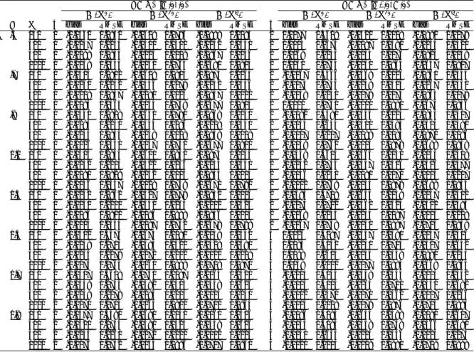
Table 1: Monte Carlo Results of the GPHF Estimation for ARFIMA(0, d, 0) Model with p = 1

d − δ ∈ [−.5, .5) d − δ ∈ [−1.5, −.5)

m = bn.5_{c m = bn}.65_{c m = bn}.8_{c m = bn}.5_{c m = bn}.65_{c m = bn}.8_c

d n τ bias RMSE bias RMSE bias RMSE τ bias RMSE bias RMSE bias RMSE

.5 150 1 -0.0009 0.3897 0.0016 0.2337 0.0006 0.1518 2 0.0767 0.5003 0.0501 0.2997 0.0224 0.1871 300 1 0.0028 0.3067 -0.0025 0.1698 0.0001 0.1055 2 0.0597 0.4359 0.0284 0.2166 0.0132 0.1355 500 1 -0.0038 0.2478 -0.0021 0.1384 -0.0020 0.0842 2 0.0367 0.3270 0.0217 0.1796 0.0120 0.1047 1000 1 -0.0034 0.2083 0.0034 0.1049 0.0002 0.0622 2 0.0347 0.2520 0.0177 0.1338 0.0058 0.0756 .7 150 1 0.0034 0.3842 -0.0048 0.2362 -0.0048 0.1529 2 0.0431 0.4967 0.0333 0.3009 0.0173 0.1885 300 1 -0.0072 0.3123 -0.0022 0.1697 -0.0019 0.1060 2 0.0402 0.4089 0.0198 0.2181 0.0134 0.1314 500 1 -0.0078 0.2512 0.0009 0.1389 -0.0013 0.0840 2 0.0301 0.3273 0.0163 0.1788 0.0076 0.1027 1000 1 -0.0003 0.2005 -0.0015 0.1062 0.0005 0.0612 2 0.0273 0.2544 0.0086 0.1294 0.0059 0.0772 .9 150 1 -0.0076 0.3818 -0.0037 0.2362 -0.0040 0.1518 2 0.0394 0.5090 0.0251 0.3058 0.0138 0.1879 300 1 0.0025 0.3038 -0.0016 0.1697 -0.0010 0.1074 2 0.0215 0.4167 0.0138 0.2135 0.0087 0.1313 500 1 0.0023 0.2476 0.0015 0.1362 0.0006 0.0846 2 0.0273 0.3204 0.0151 0.1747 0.0041 0.1030 1000 1 0.0052 0.2004 -0.0008 0.1060 0.0005 0.0622 2 0.0166 0.2551 0.0038 0.1337 0.0018 0.0746 1.1 150 1 -0.0056 0.3821 0.0076 0.2348 0.0030 0.1484 2 0.0223 0.4945 0.0152 0.3047 0.0079 0.1869 300 1 0.0013 0.3056 0.0024 0.1702 -0.0014 0.1051 2 0.0229 0.4197 0.0096 0.2177 -0.0002 0.1346 500 1 0.0027 0.2450 -0.0006 0.1380 -0.0009 0.0831 2 0.0181 0.3188 0.0066 0.1767 0.0022 0.1035 1000 1 0.0021 0.2011 0.0025 0.1060 0.0012 0.0617 2 0.0088 0.2546 0.0021 0.1330 0.0026 0.0760 1.3 150 1 0.0126 0.3879 0.0107 0.2378 0.0039 0.1499 2 0.0170 0.4961 0.0085 0.2946 0.0027 0.1875 300 1 0.0076 0.3051 0.0037 0.1676 0.0024 0.1082 2 0.0113 0.4166 0.0068 0.2206 0.0011 0.1319 500 1 0.0091 0.2490 0.0025 0.1402 0.0006 0.0820 2 0.0071 0.3312 0.0050 0.1765 -0.0000 0.1030 1000 1 0.0070 0.2018 0.0053 0.1086 0.0004 0.0613 2 0.0062 0.2556 0.0031 0.1363 0.0016 0.0758 1.5 150 2 -0.0130 0.5035 0.0025 0.2970 0.0009 0.1891 3 0.0744 0.6352 0.0454 0.3592 0.0234 0.2266 300 2 0.0003 0.4127 -0.0013 0.2141 -0.0007 0.1332 3 0.0571 0.4847 0.0314 0.2529 0.0193 0.1541 500 2 0.0035 0.3206 0.0010 0.1757 -0.0017 0.1037 3 0.0387 0.4029 0.0202 0.2039 0.0121 0.1213 1000 2 -0.0009 0.2491 -0.0019 0.1342 -0.0004 0.0766 3 0.0412 0.3193 0.0193 0.1543 0.0082 0.0886 1.7 150 2 -0.0115 0.4963 0.0030 0.2975 -0.0092 0.1871 3 0.0378 0.6265 0.0290 0.3592 0.0190 0.2251 300 2 0.0088 0.4109 -0.0086 0.2199 -0.0025 0.1319 3 0.0514 0.4894 0.0258 0.2512 0.0126 0.1577 500 2 0.0041 0.3225 0.0008 0.1752 -0.0022 0.1036 3 0.0316 0.4083 0.0202 0.2082 0.0101 0.1190 1000 2 0.0001 0.2525 -0.0003 0.1320 0.0006 0.0767 3 0.0338 0.3241 0.0140 0.1549 0.0069 0.0882 1.9 150 2 -0.0066 0.5024 -0.0014 0.3025 0.0004 0.1863 3 0.0410 0.6284 0.0203 0.3646 0.0064 0.2280 300 2 -0.0002 0.4218 0.0032 0.2123 0.0014 0.1341 3 0.0325 0.4834 0.0134 0.2534 0.0099 0.1572 500 2 0.0077 0.3217 0.0019 0.1739 0.0019 0.1033 3 0.0238 0.4065 0.0142 0.2025 0.0050 0.1194 1000 2 -0.0053 0.2544 -0.0032 0.1327 -0.0003 0.0758 3 0.0165 0.3212 0.0060 0.1552 0.0047 0.0880

a_{The data generation is (1 − L)}d_X

t= εt, εt∼ N (0, 1);

b_{The p is the pooling order;}

c_{The τ is the tapering order;}

d_{The δ, the difference order, in the expression d − δ ∈ [−.5, .5)/d − δ ∈ [−1.5, −.5) is such that for the true value d, select a δ satisfying −.5 ≤ d − δ <}

.5/−1.5 ≤ d − δ < −.5;

e_{The m is the number of the frequency ordinates involved in the estimation.}

20

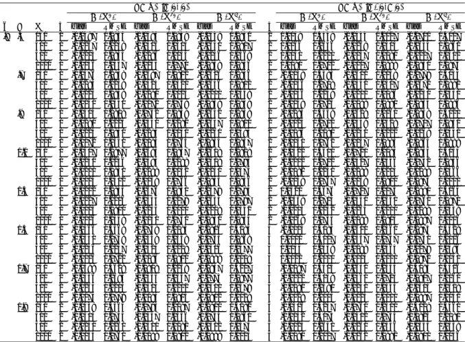
Table 2: Monte Carlo Results of the GPHF Estimation for ARFIMA(0, d, 0) Model with p = 3

d − δ ∈ [−.5, .5) d − δ ∈ [−1.5, −.5)

m = bn.5_{c m = bn}.65_{c m = bn}.8_{c m = bn}.5_{c m = bn}.65_{c m = bn}.8_c

d n τ bias RMSE bias RMSE bias RMSE τ bias RMSE bias RMSE bias RMSE

.5 150 1 -0.0097 0.3511 -0.0010 0.2006 -0.0031 0.1245 2 0.0598 0.2625 0.0582 0.2617 0.0369 0.1659 300 1 -0.0054 0.2733 0.0006 0.1396 -0.0034 0.0869 2 0.0460 0.1874 0.0401 0.1842 0.0227 0.1121 500 1 -0.0079 0.2304 -0.0017 0.1153 0.0007 0.0667 2 0.0325 0.1489 0.0313 0.1495 0.0169 0.0860 1000 1 0.0020 0.1789 -0.0007 0.0851 0.0000 0.0495 2 0.0241 0.1173 0.0215 0.1157 0.0109 0.0624 .7 150 1 -0.0091 0.3499 -0.0011 0.1979 -0.0041 0.1246 2 0.0458 0.2646 0.0400 0.2621 0.0259 0.1614 300 1 -0.0148 0.2668 -0.0027 0.1401 -0.0003 0.0869 2 0.0338 0.1854 0.0203 0.1839 0.0180 0.1096 500 1 -0.0071 0.2249 -0.0020 0.1126 -0.0021 0.0663 2 0.0243 0.1478 0.0240 0.1479 0.0112 0.0871 1000 1 -0.0026 0.1779 -0.0018 0.0828 -0.0016 0.0493 2 0.0145 0.1108 0.0142 0.1114 0.0091 0.0619 .9 150 1 -0.0082 0.3432 0.0012 0.1965 -0.0033 0.1231 2 0.0292 0.2576 0.0257 0.2571 0.0156 0.1546 300 1 -0.0061 0.2674 -0.0012 0.1379 -0.0013 0.0850 2 0.0178 0.1820 0.0205 0.1833 0.0124 0.1094 500 1 -0.0097 0.2249 -0.0027 0.1122 -0.0015 0.0665 2 0.0173 0.1432 0.0122 0.1452 0.0066 0.0852 1000 1 -0.0030 0.1723 -0.0012 0.0851 -0.0006 0.0482 2 0.0095 0.1110 0.0108 0.1106 0.0055 0.0614 1.1 150 1 0.0025 0.3470 0.0043 0.1970 0.0017 0.1253 2 0.0083 0.2504 0.0152 0.2492 0.0091 0.1507 300 1 0.0056 0.2677 0.0054 0.1372 0.0030 0.0857 2 0.0117 0.1763 0.0075 0.1754 0.0040 0.1057 500 1 0.0038 0.2231 0.0024 0.1093 0.0016 0.0647 2 0.0037 0.1451 0.0100 0.1429 0.0037 0.0832 1000 1 0.0042 0.1751 0.0004 0.0852 0.0003 0.0485 2 0.0056 0.1098 0.0045 0.1107 0.0020 0.0599 1.3 150 1 0.0307 0.3389 0.0206 0.1950 0.0141 0.1252 2 -0.0020 0.2510 -0.0012 0.2474 0.0021 0.1532 300 1 0.0259 0.2670 0.0146 0.1388 0.0100 0.0853 2 -0.0014 0.1802 0.0023 0.1749 0.0031 0.1083 500 1 0.0200 0.2244 0.0110 0.1104 0.0065 0.0666 2 0.0004 0.1425 -0.0024 0.1436 0.0009 0.0845 1000 1 0.0171 0.1750 0.0060 0.0844 0.0033 0.0488 2 0.0017 0.1090 0.0027 0.1095 -0.0007 0.0596 1.5 150 2 -0.0039 0.5700 -0.0022 0.2438 -0.0018 0.1500 3 0.0494 0.3245 0.0523 0.3228 0.0322 0.1893 300 2 -0.0071 0.3685 0.0015 0.1771 0.0004 0.1056 3 0.0439 0.2364 0.0395 0.2339 0.0228 0.1318 500 2 -0.0064 0.2925 -0.0029 0.1432 -0.0006 0.0832 3 0.0295 0.1752 0.0299 0.1760 0.0166 0.1004 1000 2 -0.0033 0.2112 -0.0015 0.1083 -0.0013 0.0594 3 0.0232 0.1358 0.0217 0.1327 0.0122 0.0729 1.7 150 2 -0.0157 0.5661 -0.0033 0.2445 -0.0039 0.1490 3 0.0468 0.3174 0.0329 0.3159 0.0186 0.1877 300 2 -0.0070 0.3615 0.0008 0.1736 -0.0012 0.1048 3 0.0277 0.2341 0.0298 0.2329 0.0175 0.1300 500 2 -0.0133 0.2881 0.0005 0.1400 -0.0020 0.0836 3 0.0211 0.1727 0.0231 0.1745 0.0108 0.0993 1000 2 -0.0031 0.2138 -0.0011 0.1058 -0.0024 0.0600 3 0.0160 0.1320 0.0138 0.1334 0.0064 0.0714 1.9 150 2 -0.0111 0.5581 -0.0055 0.2451 -0.0010 0.1530 3 0.0199 0.3174 0.0283 0.3125 0.0176 0.1839 300 2 -0.0063 0.3659 -0.0011 0.1726 -0.0009 0.1041 3 0.0233 0.2296 0.0188 0.2322 0.0099 0.1307 500 2 0.0035 0.2864 0.0017 0.1404 -0.0023 0.0827 3 0.0126 0.1712 0.0116 0.1763 0.0072 0.0973 1000 2 0.0040 0.2062 -0.0036 0.1063 -0.0014 0.0584 3 0.0101 0.1314 0.0108 0.1296 0.0034 0.0717

a_{The data generation is (1 − L)}d_X

t= εt, εt∼ N (0, 1);

b_{The p is the pooling order;}

c_{The τ is the tapering order;}

d_{The δ, the difference order, in the expression d − δ ∈ [−.5, .5)/d − δ ∈ [−1.5, −.5) is such that for the true value d, select a δ satisfying −.5 ≤ d − δ <}

.5/−1.5 ≤ d − δ < −.5;

e_{The m is the number of the frequency ordinates involved in the estimation.}

21