Ecological intuition versus economic "reason"

HAL Id: halshs-00575067

https://halshs.archives-ouvertes.fr/halshs-00575067

Preprint submitted on 9 Mar 2011

HAL is a multi-disciplinary open access

archive for the deposit and dissemination of

sci-entific research documents, whether they are

pub-lished or not. The documents may come from

teaching and research institutions in France or

L’archive ouverte pluridisciplinaire HAL, est

destinée au dépôt et à la diffusion de documents

scientifiques de niveau recherche, publiés ou non,

émanant des établissements d’enseignement et de

recherche français ou étrangers, des laboratoires

Ecological intuition versus economic ”reason”

Roger Guesnerie, Jean-Michel Lasry, Olivier Guéant

To cite this version:

Roger Guesnerie, Jean-Michel Lasry, Olivier Guéant. Ecological intuition versus economic ”reason”.

2009. �halshs-00575067�

WORKING PAPER N° 2009 - 47

Ecological intuition versus economic "reason"

Olivier Guéant

Roger Guesnerie

Jean-Michel Lasry

JEL Codes: D61, H41, H43, O4, Q2

Keywords: Discount rate, ecological discount rate,

environmental goods, relative prices, irreversible damage,

precautionnary principle

P

ARIS

-

JOURDAN

S

CIENCES

E

CONOMIQUES

L

ABORATOIRE D

’E

CONOMIE

A

PPLIQUÉE

-

INRA

48,BD JOURDAN –E.N.S.–75014PARIS TÉL. :33(0)143136300 – FAX :33(0)143136310

www.pse.ens.fr

CENTRE NATIONAL DE LA RECHERCHE SCIENTIFIQUE – ÉCOLE DES HAUTES ÉTUDES EN SCIENCES SOCIALES ÉCOLE NATIONALE DES PONTS ET CHAUSSÉES – ÉCOLE NORMALE SUPÉRIEURE

Ecological intuition versus Economic “reason”.

Olivier Guéant, Roger Guesnerie, Jean-Michel Lasry

October 28th, 2009

Abstract

This article discusses the discount rate to be used in projects that aimed at improving the environment. The model has two di¤erent goods, one is the usual consumption good whose production may increase ex-ponentially, the other is an environmental good whose quality remains limited. The stylized world we describe is fully determined by four pa-rameters, re‡ecting basic preferences "ecological" and intergenerational concerns and feasibility constraints.

We de…ne an ecological discount rate and examine its connections with the usual interest rate and the optimized growth rate. We discuss, in this simple world, a variety of forms of the precautionary principle.

Résumé

Cet article discute des taux d’actualisation à utiliser pour l’évaluation de projets visant à améliorer l’environnement à long terme. Il y a deux biens dans le modèle, un bien privé susceptible d’être multiplié de façon exponentielle, un bien environnemental,disponible en quantités limitées. Nous décrivons un monde stylisé dans lequel quatre paramètres re‡ètent les préférences entre les consommations, les considérations d’équité inter-générationnelle et les contraintes de faisabilité. Nous dé…nissons un taux d’actualisation écologique et le comparons avec les taux d’intérêt habituels et les taux de croissance. Nous discutons, dans ce monde simpli…é toute une série de formes du principe de précaution.

We thank for useful comments on a previous version Ivar Ekeland, Vincent Fardeau, Thomas Piketty, Bertrand Villeneuve and Martin Weitzman. We also acknowledge useful exchange on this sub ject with Gary Becker, Steve Murphy and Joseph Stiglitz.

1

Introduction

Environmentalists have often dismissed the economists’ approach of environ-mental problems, more especially when long term issues are at stake. On the one hand, what may be called “ecological intuition” puts high priority on the long run preservation of the environment. On the other hand, the cost-bene…t analysis promoted from economic reasoning calls for the use of discount rates that apparently lead to dismiss the long run concerns. The climate issue is the most recent avatar of the clash between “ecological intution” and “economic reason”: in sharp contrast with most environmentalists and many climatolo-gists’ sensitivity, the computations based on Nordhaus (1993) suggest lenient climate policies. And although Nordhaus has made cautious warning, some of his less cautious readers (Lomborg (2001)) claim that their …ght against climate policies proceeds from “economic reason”. Although the Stern review (2006) has changed the tone of the debate, it is clear that Stern’s views of “economic reason” and of the subsequent cost-bene…t analysis, is not broadly accepted in the profession.

The present paper attempts to retackle the clear antagonism between the two sides from a simple model, that has been recurrently evoked in the economists’ debate, (see Krautkramer (1987), Heal, (1998)) but the relevance of which in the present debate has been recently more systematically stressed by Guesnerie (2004) and Hoel and Sterner (2007) and Sterner and Persson (2007). The model assumes that there are two goods at each period: the environment, a non-market good available in …nite quantity and standard aggregate consumption, which is allowed to grow for ever. The opposition between a …nite level of environmental good and an increasing level of consumption good echoes a core determinant of the “ecological” sensitivity: sites, lands, seashores, species are …nitely available on the planet. On the contrary, modern optimism, based on the “economics” of past growth performance, leads to believe that consumption of the so-called private goods may be multiplied without limit.

We discuss the long run cost-bene…t analysis issues that arise within a model, that has indeed two goods, the two goods being associated with aggregate con-sumption and aggregate environmental quality. As emphasized in Guesnerie (2004), in such a setting, cost-bene…t analysis has to stress, not only the stan-dard discount rates but also, the “ecological” discount rate, the evolution of which re‡ects the relative price of environment vis à vis the standard private good1_{. The simple in…nite horizon world under scrutiny is entirely described by}

four parameters.

The …rst parameter describes how substitutable are the standard and envi-ronmental good in producing welfare. Opinions on the value of this parameter may di¤er and lead to oppose a “moderate” environmentalist and a “radical” environmentalist. The second parameter is the classical elasticity of marginal utility which allows to assess the extent to which welfare is subject to satiety,

1_{It is well known that in an n-commodity world, there are as many discount rates as there}

and which classically determines the intertemporal "resistance to substitution", or in a risky context, "relative risk-aversion".The third parameter is a pure rate of time preference which, in this setting measures, the degree of intergener-ational altruism of the agents. The last parameter is an interest rate which in the logic of a simple endogenous growth context (of the AK type) indicates to which extent one can transfer consumption between periods and generations. It is here a su¢ cient statistics for describing the intertemporal production possibilities. . Within this model, the research agenda is most clear: we have to under-stand how the various parameters under consideration a¤ect the trade-o¤ be-tween present and future consumption, whether it is standard or "environmen-tal" consumption. In the latter case, the trade-o¤ is re‡ected in the "ecological" discount rates supporting the optimal policy: its values allow to stress in a some-what synthetical way, the di¤erence between the “moderate” and the “radical” ecological viewpoints.

The paper proceeds as follows.

Part 1 of the paper presents the basic model, but abstract from the "feasi-bility" constraints, by putting emphasis on an exogenous growth path of private consumption: it adopts the "reform viewpoint" which provides a good introduc-tion to the optimizaintroduc-tion approach of Part 2.

Part 2 indeed characterizes the optimal growth policy under the assumption that environmental quality remains constant over time. The analysis allows to derive both the time pattern of optimal growth rates of private consumption and of the "ecological discount rates". It leads to put emphasis on di¤erent "yield" curves.

Part 3 attempts to answer a number of questions relating with the so-called precautionary principle: how much should the present generation be willing to pay to avoid an irreversible damage to the environment that will take place soon or on the contrary at some later date ? The question makes sense in a deter-ministic context where the nature and extent of the damage is well ascertained ex-ante. When the scienti…c evidence is lacking, the damage has to be viewed as uncertain: such an uncertainty, that will be ex-post truly revealed, is re‡ected here in di¤erent ex-ante evaluations of the environmental concern made by the moderate and the radical environmentalist. We stress three versions of the extent of "precaution" imbedded into our analysis. The …rst one stresses the maximal willingness to pay of a society for avoiding a deterministic irreversible damage. When damages to-day are truly uncertain, we stress …rst a "weak precaution-ary principle", which is reminiscent when "ecological" discount rates matter of Weitzman’s classical argument (2001) on long run standard discount rates, and, second and …nally, a strong "precautionary" principle, which we view as the most striking result of this paper.

The connections of the paper with the literature are as follows. Models with two-goods include Heal (1998). The model of the paper is the one considered in Guesnerie (2004), and the argument exploits the …ndings of this paper. It also uses some of the insights of Hoel-Sterner (2007) and Persson-Sterner (2007), who have examined the same model and, mainly in Part 2, some further insights of Guéant-Lasry-Zerbib (2007). All these papers refer to the concept of “ecological

discount rates” emphasized in Guesnerie (2004), a concept that has also been stressed in a somewhat more complex setting than ours, and with a di¤erent focus, by Gollier (2008). Note also that the importance of substitutability, which we emphasize here, has been stressed earlier in Neumayer (2002) and Gerlagh-Van der Zwann (2002).

Note that the views presented here on discounting and precaution have a motivation closely connected to the one of Weitzman (2009). However our emphasis is on relative prices e¤ects: even if we put emphasis on the uncertainty that surrounds the long run environmental issues and on the weight to be put on the bad case, we do not stress "fat tails".

Part I

Model and preliminary insights.

1.1

Goods and Preferences.

We are considering a world with two goods. Each of them has to be viewed as an aggregate. The …rst one is the standard aggregate private consumption of growth models. The second one is called the environmental good. Its “quantity” provides an aggregate measure of “environmental quality” at a given time. It may be viewed as an index re‡ecting biodiversity, the quality of landscapes, nature and recreational spaces, the quality of climate, the availability of water2_.

We call xt the quantity of private goods available at period t, and yt the

level of environmental quality at the same period. Generation t, that lives at period t only, has ordinal preferences, represented by a concave, homogenous of degree one utility function:

v(xt; yt) = h x 1 t + y 1 t i 1

However, the measurement of cardinal utility, on which intertemporal judge-ments of welfare will be made, involves an iso-elastic function.

V (xt; yt) =

1

1 0v(xt; yt)

1 0

The above modelling calls for the following comments that concern respec-tively v and V:

Concerning v; we have to stress several points, the …rst two ones concerning the symmetry of the model.

2_{As we shall do in a companion paper later, we may view it, in a broader way, as integrating}

many non-markets dimensions of welfare, for example the non-market costs of migrations, health problems relating to climate change.

The reader has noted that both xtand ytappear with the same coe¢ cient

in the function v. However this is without loss of generality for exam-ple as soon as we keep control of the freedom in the measurement3

of yt.

Giving the same weight to the private good index and to the environ-mental quality index is a matter of notational convenience. However, leaving this weight constant across time, and in fact, what matters non vanishing, is a substantive assumption. It implies in particu-lar that the concern for environmental goods does not shrink, as it would in a world where all private and environmental goods would be symmetric and where the number of private goods would increase inde…nitely. The present assumption on the symmetric role of x and y is intended to re‡ect the fact that we “only have one planet”, the preservation of which is not, and will never be, a point of minor concern for its inhabitants, whatever their ability to produce large quantities of new private goods. Even, if the speci…c modelling is crude, this point seems well taken for our purpose in the sense that we do not deny a priori the soundness of “ecological intuition”. A CES utility function, where is the elasticity of substitution, describes

a speci…c pattern of substitution, which is special but easy to grasp. As the reader will easily check, a key insight into the present formula-tion is the following: the marginal willingness to pay - in terms of the private good - for the environmental good is (@2V )=(@1V ) = (x=y)1= .

This can be viewed as the implicit price of the environmental good. When the ratio environmental quantity (here quality) over private good quantity decreases by one per cent the marginal willingness to pay for the environmental good, or its implicit price, increases by ( 1= ) per cent. Equivalently, looking at compensated choices, i.e. substitution along an indi¤erence curve we see that when the ratio of the (implicit) price of the environmental good over price of the private good decreases by one per cent, then the ratio quantity (here quality) of the environmental good over quantity of the private good increases by per cent. It follows that if, as we often suppose in the following, environmental quality is constant and equals y; and the private good consumption increases at the rate g; then the mar-ginal willingness to pay for the environmental good increases at the rate (g= ); which is greater (resp. smaller) than g; if is smaller (resp. greater) than one. Let us remember also that existing studies

3_{Indeed, as we shall see later, one can de…ne at each period a “green GDP”, (the product}

of the implicit price of the environmental good by its quantity) and the standard GDP, (the product of the quantity of private goods by its price). The ratio of green GDP over the standard GDP is indeed, see below, (yt

xt)

1 1

, and, once we know , we may calibrate the model, i.e. choose the units of measurement of the environmental good by assessing the relative value of green GDP at the …rst period. This analysis would however have to be quali…ed in the limit Cobb-Douglas case ( = 1) where the share of green GDP vis à vis standard GDP does depend on the coe¢ cient of the Cobb-Douglas function.)

on environment often suggest that it is a “luxury” good in the sense that the marginal willingness to pay increases more than wealth or income. Now, the number y x

y

1

may be called the ”green” GDP: note that it grows inde…nitely whenever x grows inde…nitely, if, as we suppose here, y remains …nite. Note also that the ratio of ”green” GDP over standard GDP is = y_x 1

1

and the ratio of green GDP to total GDP is: =₁₊ .

Let us come to V . The marginal utility of a “util”of v, takes the form v 0: when v increases by one per cent, marginal cardinal utility decreases by 0 per cent. This is the standard coe¢ cient linked to intertemporal elasticity of substitution (1

0), relative risk aversion ( 0) or intertemporal resistance

to substitution.

1.2

Social welfare

Social welfare is evaluated as the sum of generational utilities. In line with the argument of Koopmans, we adopt the standard utilitarian criterion:

1 1 0 +1 X t=0 e tv(xt; yt)1 0

Two comments can be made:

The coe¢ cient is a pure rate of time preference. Within the normative viewpoint which we mainly stress here, the fact that this coe¢ cient is pos-itive has been criticized, for example by Ramsey who claims that this is “ethically indefensible and arises merely from the weakness of the imagina-tion”or Harrod (1948) who views that as a “polite expression for rapacity and the conquest of reason by passion”. Reconciling these feelings with Koopmans’argument4 _{leads however to accept a positive and small , the}

smaller, the more “ethical considerations become preponderant”: along the "ethical" line of argument, it has been argued that the number might be viewed as the probability of survival of the planet5_.

We may view the coe¢ cient 0, as a purely descriptive one, re‡ecting intertemporal and risk behavior, or as a partly normative coe¢ cient, re-‡ecting the desirability of income redistribution across generations. This is the more frequent interpretation we stress in the paper: a low (resp. high)

0 _{re‡ects little (resp. a lot of) concern for intergenerational equality.} 4_{“Overtaking” would be another, di¤erent, way to proceed.}

5_{This argument is more satisfactory when we model adequately the uncertainty of the}

problem. Within a deterministic framework, a higher may sometimes be a proxy for the inappropriate treatment of uncertainty.

At this stage, something more can be said on the philosophy of the approach taken here.

We have adopted a stylized description of the trade-o¤ between environmen-tal quality and private consumption. We recognize that the modelling of the trade-o¤, (depending at every period on a single parameter, and more impor-tantly, the same across time), is crude. However if the degree of substitutability between standard consumption good and environment is …xed, we leave its value open. At this stage, we do not decide whether is smaller, a plausible short run hypothesis6_{, or greater than one, and we leave it …xed. We associate a high ,}

(resp. low ) to a moderate, (resp. radical) environmentalist’s viewpoint, the dividing line being obviously = 1.

At this stage, one should give some insights on the qualitative di¤erences between the cases > 1 and < 1, i.e. between the opinions we attribute respectively to the ”moderate” and the ”radical” environmentalists. These dif-ferences echo the views that shape the understanding of the future long run usefulness of environmental quality when compared to private consumption.

We have:

v(xt; yt) = xt[1 + (

yt

xt

)( 1)]( 1)

First, let us consider > 17. Now, v grows as xtwhenever _xyt_t tends to zero

and social marginal utility of consumption will decrease at 0 times the growth rate of v, which is the growth rate of consumption. The asymptotic relative contribution of environment to welfare is vanishing and similarly, the Green GDP becomes small when compared to standard GDP. As we shall see later recurrently, the moderate environmentalist is very moderate in the long run.

On the contrary, in the case where < 18_{, it is useful to write:}

v(xt; yt) = yt[1 + (

yt

xt

)(1 )]( 1)

In that case, (reminding that ₁ < 0), v does not grow any longer indef-initely with xt, but tends to y. Then, social marginal utility of consumption

tends to zero as x 1= _(y1= 0_{) that is at a speed independent of} 0_{. The}

in-crease in the consumption of private goods still contributes to welfare but with an asymptotic limit associated with the level of environmental quality. Stan-dard GDP becomes small with respect to Green GDP.

6_{Since, again, the marginal willingness for environmental amenities seems to grow faster}

than private wealth. (see Krutilla J. Cichetti C. (1972))

7_{For example, with = 2}

v(xt; yt) = xt[1 + (yt xt )(1=2)]2 8_{For = 1=2,} v(xt; yt) = yt[1 + ( yt xt )]( 1)

We will argue later that the problem under scrutiny is dominated by uncertainty, and that such an uncertainty is decisively re‡ected in our framework through what is, in our stylized framework, the summary statistics of the desirability of a good environment, i.e. the parameter . At this stage, we focus attention on the deterministic cases and emphasize the di¤erences. First, it is useful to search for some intuition of the argument, by understanding what goes on at the margin of some economic trajectory. We shall then look at the intertemporal social optimum in a most elementary endogenous growth model.

2

Preliminaries: Investigation around a simple

reference trajectory.

2.1

The reference trajectory, …rst de…nitions and insights.

In order to give some intuition on the question of discount rates, we shall con-sider a reference trajectory of the economy where environmental quality is …xed at the level y and where the sequence of private goods consumption denoted x_t is also given (we often assume that the growth rate g of consumption is itself …xed). Note that our formulation, at least at this stage, does not assume either “limits to growth” due to the …nite ecological resources nor even deterioration of the ecological production due to growth.

The question we examine is: what are the discount rates, standard interest rate for private goods, i.e. the return to private capital rt, and what we call the

ecological rate for environmental goods implicit to the …xed trajectory ? We shall …rst investigate the implicit discount factors at the margin of our reference trajectory, with …xed environmental quality and exponential growth. We sometimes refer to this approach as the “reform” viewpoint. In the next section, we shall then take the optimization viewpoint and stress connections between the present reference trajectory and a socially optimal trajectory.

The reference trajectory has consumption growing at the rate g_t (by de…-nition x_t+1= egtx

t) and the environmental quality equal to y.

We want to compute the implicit discount rates that sustain this trajectory, that is the discount rates that make it locally optimal.

De…nition 1 The implicit discount rate for private good between periods t and t + 1, is r_t such that e rt _{= e} @1V (xt+1; y) @1V (xt; y) where @1V (x; y) = h x 1 + y 1i( 1 0 1 ) x 1:

The discount rate between periods 0 and T is then classically de…ned as : R (T ) = 1

T

T_X1 t=0

The discount rate R (T ) tells us, as is standard, that one unit of consumption at period t, is (socially) equivalent to e T R (T )today.

We introduce the ecological discount rate, which as stressed in Guesnerie (2004), is the discount rate speci…c to the commodity environment9_.

De…nition 2 The ecological implicit discount rate between two consecutive pe-riods is _t de…ned by:

e t _{= e} @2V (xt+1; y)

@2V (xt; y)

The discount rate between periods 0 and T is: B (T ) = 1

T

T_X1 t=0

t

The ecological discount rate tells us that one marginal improvement of en-vironment today is socially equivalent to e T B (T ) _{of the same improvement}

occurring at period T . It implies that the present generation, when viewing an improvement of environment occurring at period T , (improvement supposed, for example, to be triggered by some present spending), should compare the present cost with the discounted value, (discounted with the ecological discount rate), of the present marginal willingness to pay for the same improvement today. (This is what is called “standard”ecological cost-bene…t analysis by Guesnerie (2004)). In other words, the cut-o¤ maximal cost that the society is willing to incur for a unit improvement of the environmental quality at period T , i.e. e T B (T )_{C (0)}

where C (0) is the willingness to pay of the present generation (indeed here, (y(0)=x(0)) 1= _{) for the same unit environmental improvement.}

2.2

Implicit discount rates along the reference trajectory.

We can now provide explicit formulas for our implicit discount rates along the reference trajectory that has been introduced.

Proposition 3 Along our reference trajectory, x0; : : : ; xt+1= egtxt; : : :

the implicit private discount rate for the private good between periods t and t + 1 can be equivalently written as,

either: r_t = + g_t 0₊1 0 1 ln 1+ t 1+ _t+1 or r_t = + g_t= +1 ₁0ln 1+ t 1 1+ _t+1 1 where _t = yt@2V xt@1V = xt yt 1 ₁ is the ratio of Green GDP over standard GDP.

9_{Hoel-Sterner(2006) consider the same model as here or as in Guesnerie (2004), without}

The ecological discount rate between periods t and t + 1 is:

t = rt gt=

The …rst formula shows how the standard logic of discount rates (r_t = + g_t 0_{) is a¤ected by the environmental concern. The correction depends on}

ratios that depend upon _t, a coe¢ cient that may be viewed as the ratio of Green GDP over standard GDP and _t is its value along the trajectory. The second formula looks strikingly di¤erent from the …rst one, although it is equivalent, but it puts emphasis on factors that become dominant in one of the case under scrutiny later.

Indeed, one can get a more informative and balanced view of the two …rst formulas, by taking a …rst order approximation, (justi…ed if the time period is small) of the expression r_t = + g_t 0₊1 0

1 ln 1+ t

1+ _t+1 .

Corollary 4 A …rst order approximation of the preceding formula is: r_{t '} + g_t(₁₊1

t

0₊ t

1+ t

1₎

A similar formula was indeed stressed by Hoel and Sterner (2006) who con-sidered the continuous time version of the model10_.

The third formula stresses the e¤ect of the growth of private consumption on the ecological discount rate: it is qualitatively unsurprising that it is connected to the standard discount rate with a negative correction that increases with the growth rate and decreases when the elasticity of substitution increases. This formula, which captures the relative price e¤ ect that we are stressing here is particularly simple and intuitively appealing. We can think about it as follows: it would be equivalent to give up one unit of environmental quality at the present period t, in order to provide e t of environmental quality tomorrow, but the

suggested move is equivalent, from the view point of both generations, to give up C(t) units of private goods and to provide C(t)ert _{units, as soon as C(t)e}rt

compensate for one unit of environmental quality at time t+1, which is the case, if and only if C(t)ert _{= C(t + 1)e} t _{= C(t)e}gt= _e t_{. The conclusion follows and}

stresses a key ingredient for the understanding of the argument of the present paper.

The dynamics of the implicit discount rates stressed above is related to the dynamics of the growth rates. We will not examine this question comprehen-sively here, but will only focus it on the long run behavior of the discount rates, under the assumption that the average growth rate of consumption converges:

1 T

PT 1

t=0 gt ! g .11

1 0_{Recently Gollier(2008) has derived generalizations of these formulas to general utility}

functions with uncertainties on g and y, in a similar world with two goods.

1 1_{Standard optimization à la Ramsey-Solow, with exogenous technical progress, does not}

necessarily lead to an asymptotic growth rate. (for a review on these issues, see Guesnerie-Woodford (1992)). We reconsider this problem in the special endogenous growth model that will be studied from the next Section.

We focus our attention on the long run discount rate for private good, i.e. the limit of the discount rate between periods 0 and T , R (T ) = _T1 PT_t=01rt,

when T becomes high. Similarly, the long run ecological discount rate is the limit, when T increases inde…nitely of B (T ) = 1

T

PT 1

t=0 t:

The next result, again a corollary of Proposition 3, stresses the spectacu-lar di¤erences in the behavior of long run discount rates, according to whether

> 1 or < 1

Corollary 5 _{At the margin of the reference situation, when T tends to +1,} - When > 1,

R (T ) ! + g 0 _{and B (T ) ! + g (} 0 _{1= )}

- When < 1,

R (T ) ! + g = and B (T ) !

This proposition, stressed in Guesnerie (2004) provides a useful introductory key in the the problem. Here are some comments:

In the …rst case ( > 1), the traditional case in the sense that the two goods are good substitutes, standard considerations matter for the standard long run discount rate, while however, the limit value of the ecological discount rate is signi…cantly below the value of the standard discount rate (the di¤erence is given by g= ).

The second case ( < 1) is characterized by a low substituability between the private good and the environmental good. For the reasons analyzed above, the qualitative logic underlying the standard discount rate is en-tirely changed and the value of the asymptotic ecological discount rate only depends on and not on the growth path.12

The result suggests strong asymptotic discontinuity between the cases < 1 and > 1 when the same rate of growth of consumption is inserted in the formulas. In a sense this is not surprising since it has been known for long that CES modelling involves a discontinuity when the elasticity of substitution goes through 1 (see Arrow-Chenery-Solow (1961)). Indeed, this result does not depend on our assumption of time stability of ;but on its asymptotic limit, as shown by the next proposition.

Proposition 6 If limt!+1 t = 6= 1 then, at the margin of the reference

situation, when T tends to +1, the above asymptotic results on discount rates do depend on > 1 and < 1 in an unmodi…ed way. The case where t! 1 is

undetermined and depends, among other things, on the convergence speed.

1 2_{A long run value of < 1, means that the environmental issues become preponderant in}

the long run: indeed the situation was characterized by “ecological strangling” in Guesnerie (2004)).

We shall come back below, in Section 2-1, on the economic signi…cance of the discontinuity13.

At this stage, it should however be stressed that the exact relevance of the comparative statics analysis of the long run discount rates is unclear. It goes without saying, for example, that there is a priori no reason to refer to the same growth rate of consumption under di¤erent assumptions on , since these assumptions re‡ect di¤erent views, (moderate or radical) of the contribution of the environment to welfare, and then potentially very di¤erent views on desirable growth. In the next section, we will indeed leave these di¤erent views be re‡ected in di¤erent choices of growth rates of consumption.

Part II

Optimized growth: the evolution

of private consumption and of

"ecological" discount rates.

The above results hold at the margin of any trajectory, whether it is non-optimal, or optimal either in a …rst best sense or in a second best sense. However, as just argued the a priori drastic disagreements on the relative contribution of the private consumption and environmental consumption, involved in the choice of , makes unclear how di¤erent the choices of consumption trajectories will be a¤ected by , so that the “reform” assessment of the di¤erences may be misleading.

To go further, we stick to the option of a …xed environmental quality, but put emphasis on the endogeneity of private consumption: we then compare choices in general and ecological discount rates, in particular, not from arbitrary growth trajectories but from optimized trajectories. We choose the simplistic endogenous setting of the AK type, where the interest rate r is exogenous, being then a one-dimensional su¢ cient statistics of the intertemporal production possibilities14_{. Hence, as announced in the introduction, our discussion within}

the model will focus on four parameters only, one associated with the ecological concern, , a second one with a standard dimension of preferences 0_{, the third}

one with "ethical" considerations and the last one r with economic constraints:

1 3_{Now, let us furthermore note that the case = 1is neither the limit of < 1nor of}

> 1. Indeed, one proves that, if = 1, at the margin of the reference situation, when T tends to +1, R (T ) ! +12g ( 0+ 1)and B (T ) ! +

1

2g ( 0 1).

1 4_{Note that such an interest rate r can be extracted from a research arbitrage equation (as}

3

The model and characterization of the social

optimum.

3.1

Characterization results.

Our viewpoint is normative, and we refer to the intertemporal social welfare function introduced above. The “social Planner” maximizes:

1

X

t=0

e tV (xt; yt)

Our modelling choice of the AK type leads to consider the following economic and environmental constraints:

Economic constraints: t+1 = er( t xt) where t stands for the wealth

at date t15_.

Environmental constraints: The environmental quality is limited to y that is: yt y:

We naturally assume that r > : Furthermore, in this model, it is easy to check that optimization would lead to an in…nite postponement of consumption if r(1 0_{) > . We rule this out and assume that} 0 _{> 1 ( =r). This}

means, given the order of magnitude that we have in mind, that we will consider that 0 is essentially greater than 1.

The next proposition gathers all the asymptotic results of social optimiza-tion. The …rst part stresses that optimality requires asymptotically constant growth whatever the parameters under scrutiny. However, both the asymptotic economic growth rates and the long run ecological discount rates crucially de-pends on the value of and 0_:

Proposition 7 - At the optimum, the private goods consumption grows asymp-totically, whatever ; 0_.

- The optimal asymptotic growth rate for the private good x_t depends on and is given by the following formulae:

- If < 1 then g₁= (r ) . - If > 1 then g₁= r 0 16

1 5_{A slightly more sophisticated version allows}

t+1= exp(r)[ t xt+ wt], where tstands

for the wealth at date t and wt is a possible exogenous production ‡ow that introduces no

binding constraint into the analysis.

1 6_{The case = 1is speci…c and then g}

1=

2(r ) 1+ 0 .

- The asymptotic ecological discount rate, associated with the socially optimal trajectory is B₁= limT!+1B (T ) given by the following formulae17:

- If < 1 then B₁= . - If > 1 then B₁= (1 1

0)r + 10 .

The proof is in the appendix: once the regular asymptotic behavior of the growth rates is established, the results can be obtained from the formulas derives in the preceding section. Let us comment on the key insights.

The …rst one refers to the standard intuition as soon as > 1. The as-ymptotic growth rate of consumption is r 0 , …tting the standard formula of the

one-good model: the presence of the environmental good is asymptotically irrel-evant (although it is relirrel-evant on the optimal trajectory). The result for the other case ( < 1) may be surprising for two reasons: …rst, it was, a priori, unclear that the “radical”environmentalist would choose a positive asymptotic growth. The second point is more surprising: under the assumption that 0 _{> 1, even}

if the asymptotic growth rate chosen by the radical environmentalist relates in an expected way with the preference for the environmental good (it decreases when gets lower), it is still greater than the one chosen by the moderate en-vironmentalist. Note however that the conclusion will be easily reversed once we suppose, as it is clearly the case, that growth may a¤ect negatively environ-mental quality. The reader will …nd the intuition of both facts by returning to the above explanation of the long run di¤erences of views between the “radical” and the “moderate” environmentalist.

Nevertheless, the opposition between the “radical”environmentalist and the “moderate” one remains clearly stressed through the behavior of the ecological discount rate. The asymptotic di¤erence is again spectacular, as shown if we plot the asymptotic ecological interest rate as a function of :

1 7_{If = 1then B}

1= 1

0

Figure 1: Dependence on of the variable B₁when 0 = 2

Again the asymptotic results stress a discontinuity in the world around = 1: However, this discontinuity may be seriously quali…ed.

Proposition 8 At each period T, the optimal trajectory, is a continuous func-tion of the parameters ; 0_:

In a sense, the discontinuity associated with = 1 is worrying and might be viewed as an objection18to our (admittedly crude) modelling choice. The above continuity result, which says that at a given period results are continuous func-tions of , weakens the objection: the discontinuity “in the limit”is compatible with continuity “at the limit”: indeed B (T ) is a continuous function of when T is …xed (and …nite), as stated in a Corollary.

Corollary 9 _{8T < 1; 7! B (T ; ) is continuous.}

All these results suggest to put the emphasis on the trajectory and to stress the time paths of discount rates. This will be done later but let’s …rst concentrate on a variant of the model in which the environmental quality decreases instead of being constant.

3.2

The case of environmental good exhaustion

We have stressed the polar case of …xed environmental quality. The opposite po-lar case is the exhaustion of the environmental good at a rate g0 _{(deterioration}

means a positive g0_{, although formally it may be negative if the environment} 1 8_{Or an appropriate modelling option, since it suggests that a possible catastrophic change}

improves). This means that the condition yt = y is replaced by yt = ye g

0_t

.

Proposition 10

- At the optimum, the private goods consumption grows asymptotically, what-ever ; 0_.

- The optimal asymptotic growth rate for the private good x_t depends on and is given by the following formulae:

- If < 1 then g₁= (r ) g0₍₁ 0₎

- If > 1 then g₁=r 0 19

- The asymptotic ecological discount rate, associated with the socially opti-mal trajectory is B₁= limT!+1B (T ) given by the following formulae20:

- If < 1 then B₁= 0_g0_.

- If > 1 then B₁= (1 10)r + 10

g0

.

Note that if one interprets as a rate of survival of the planet, even a small rate of decrease of the environmental quality (let us say smaller than this survival rate if 0 _{> 1) would make the long run ecological discount rate negative, as}

soon as < 1. In the case > 1, the ecological discount rate will be a¤ected without being negative.

3.3

The dynamics of ecological discount rates

Here, we are focusing attention on the evolution of ecological discount rates with time, and what can be called yield curves for ecological discount rates B (T ).

Since B (T ) = r 1 1_T PT_t=01g_t, the dynamics of the ecological discount rate is linked to the dynamics of growth. Indeed, the dynamics of optimal growth can be assessed here.

Proposition 11 g_t converges monotonically toward its limit according to the following rules:

- If 0 _{> 1 (resp.} 0 _{< 1) and < 1 then g}

t is increasing (resp. decreasing)

- If 0_{> 1 (resp.} 0_{< 1) and > 1 then g}

t is decreasing (resp. increasing)..

- If = 1 or 0 _{= 1 the optimal growth rate is constant.}

Now using the formula B (T ) = r 1 1 T

PT 1

t=0 gt, we can deduce the shape

of the yield curve for ecological discount rate:

1 9_{The case = 1is speci…c and then g}

1= 2(r ) 1+ 0 . 2 0_{If = 1then B} 1= 1 0 1+ 0(r ).

Corollary 12 The shape of the yield curve is the following:

- If 0 > 1 (resp. 0 < 1) and _{< 1 then T 7! B (T ) is decreasing (resp.} increasing) and converges towards .

- If 0 _{> 1 (resp.} 0 _{< 1) and > 1 then T 7! B (T ) is increasing (resp.}

decreasing) and converges towards 1 1

0 r + 10 .

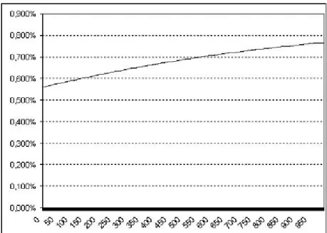
To illustrate our proposition, we drew yield curves using a simulation of the growth path21_{. Two examples, in the case} 0 _{> 1 are given below where the}

x-axis represents years and the y-axis the value of the ecological discount rate. As it comes from the previous statements, in the …rst case ( < 1 and

0_{> 1), the yield curve is decreasing and converges towards .}

In the second case ( > 1 and 0 _{> 1), the yield curve is increasing and}

converges towards r r 0.

Figure 2: Yield curve example ( = 0:8, 0_{= 1:5, r = 2%, = 0:1%)}

Figure 3: Yield curve example ( = 1:2, 0_{= 1:5, r = 2%, = 0:1%)}

The diagrams suggest that ecological discount rates converge slowly to their asymptotic value. Another interesting and related visual insight is that, when is low, the rate is low, but, even when is high, because the curve is in-creasing, the environmental rate is still low in the medium run. Hence, what the diagrams show is that, for a time period between 1 and 3 centuries from now, the disagreement between the moderate environmentalist and the radical environmentalist is not huge: both have an ecological discount rate signi…cantly below 1%; the …rst one is between 0:6% and 0:65% and the second one is be-tween 0:25% and 0:20%. Their willingness to pay, for let us say a generation living at date 150 equals the discounted value, with the ecological discount rate, respectively roughly 1=2 and 3=4, multiplied by their own marginal willingness to pay, which itself depends on their wealth and on their “ecological” views or intuition. We investigate these points below.

3.4

Pro…table “ecological”investment, horizon and wealth

The ecological discount rate, as any commodity discount rate, tells us how to compare the environmental bene…ts to present generation and the environmental bene…ts to future generations. The marginal willingness to pay for one environ-mental improvement, let us say a unit environenviron-mental improvement, at date T is B (T ) (the ecological discount rate) multiplied by the present marginal will-ingness to pay for the improvement, i.e. (x0

y)

pay is correlated with wealth (proportional to wealth when = 1 and convex or concave in wealth otherwise, depending on whether is greater or smaller than 1).

We are going to go further in the understanding of the e¤ect of wealth on the propensity to invest in “ecological” devices.

Let us then de…ne the ecological “return” of a unit cost initial investment that has the unique e¤ect of triggering an improvement of the “ecological” quality at T, as = e (T )T_{: Such an investment is just pro…table socially if}

e B (T )T_e (T )T₍x0

y )1= = 1, so that (T ) = B (T ) ( 1

T)(1= ) ln(x0=y).

Equivalently, using the ratio of green GDP over standard GDP, we may rewrite the formula: (T ) = B (T ) (_T1)(₁1 ) ln( ₀):

If we de…ne ₁ by limT!1 (T ) then:

1= B1

Hence (T ) is the ecological return of a just pro…table unitary initial investment. Equivalently, it allows to express the relative price of the environ-mental good at time T, in terms of the private good price at time 022. With this interpretation in mind, we construct the cut-o¤ “ecological return” curves T 7! (T ). We see that these curves di¤er from the ecological discount rate curves by a term in 1=T , which depends on the wealth of the economy, and the sign of which varies with this initial wealth.

Below, we have visualized several such “yield” curves that follow from the combination of the wealth e¤ect with the e¤ects discussed above (depending on

and 0_).

The required “return”, in terms of environmental quality, of a one-unit in-vestment is, in the long run, the same for a poor country and a rich country, but the …gures provide a striking illustration that, in the short run, a rich coun-try can a¤ord negative such returns, (…gure 4) when a poor councoun-try requires positive and rather high such “returns” (…gure 6).

2 2_{The standard discount rate allows to compare the relative price of the private good at}

times T and 0, whereas the ecological discount rate allows to compare the relative price of the environmental good at times T and 0.

Figure 4: Yield Curve for ( = 0:8, 0_{= 1:5, r = 2%, = 0:1%, y x} 0)

Figure 5: Yield Curve for ( = 0:8, 0_{= 1:5, r = 2%, = 0:1%, y ' x} 0)

Figure 6: Yield Curve for ( = 0:8, 0= 1:5, r = 2%, = 0:1%, y x0)

4

Precaution

The precautionary principle refers to the desirable action to be taken in order to avoid an "irreversible damage to the environment". We can examine the question in our model. We …rst consider the case where the "irreversible dam-age to the environment" is imminent and well ascertained. However one of the most popular statement of the precautionary principle stresses the uncertainty surrounding the so called damage: "Where there are threats of serious or irre-versible damage, lack of full scienti…c certainty shall not be used as a reason for postponing cost-e¤ective measures to prevent environmental degradation." The question of the right intensity of action for implementing "cost-e¤ective mea-sure" seems however to be left open. The present section indeed provides the tools for implementing a cost-bene…t analysis of the desirability of precaution.

4.1

Valuing an irreversible damage to the environment.

The question we raise here is simple: consider a damage to the environment that would take place today. In order to avoid this damage for itself, the present generation is willing to pay x. How much should it be willing to pay if this damage not only occurs now but is irreversible, i.e. if it deteriorates the well-being of all future generations ? Let us call mx the willingness to pay for the fact that the damage is irreversible, instead of x the price paid when the damage

is temporary (one period23) and only concerns the present generation.

Avoiding the damage can then be viewed as providing kind of x ecological perpetuities, the price of which is mx (this would be the price of x …nancial perpetuities, priced with a constant interest rate 1

m)

We provide here lower bounds on m.

Theorem 13 Let’s introduce a = max ; r(1 1

0) + 10 .

In the present deterministic context, if the initial generation is willing to pay x in order to avoid a temporary (here one year) damage, it is willing to pay mx to avoid making it irreversible, where the number m is greater than 1_a

The …rst remarkable feature of the theorem is that the lower bound to m, is valid both for > 1; and for < 1. However, there are still two results depending on 0 7 1. If 0 > 1 then, since < r, a = r(1 10) + 10

whereas if 0< 1 the result is simply that m 1 since a = in this case. It is also remarkable that m does not depend on initial wealth, although, initial wealth determines x, and hence the to-day willingness to pay for avoiding the considered damage.

Let us note that if the planner neglected the relative price e¤ect associated with the increase in relative desirability of the environmental good, the discount rate would be r and m would be approximately 1

r(approximately because we use

an exponential discounting) as for a classical perpetuity. Hence, the introduction of the environmental good can drastically change the willingness to pay of the present generation for an environmental or ecological perpetuity that protects all future generations from an irreversible damage. For instance, if we consider that _{' 0, then m is, in our deterministic study with}24 0 _{> 1, greater}

than the "naive" assessment 1_r, the multiplier being ₁ 11

0. If you consider

the parameters values associated with the above graphs ( 0 _{= 1:5), instead of}

having m ' 20 (resp. m ' 50) for r = 5% (resp. r = 2%), we get when = 0:8;

m 6 20 = 120 (resp. m 300) and with = 1:2, m 2:25 20 = 45 (resp.

m 112:5)

In order to get some idea on the quality of the bounds obtained in the above theorem, we provide the computations of actual m, …xing now the other common parameters at y = 1, r = 3%, = 1% and 0= 1:5, in two cases that correspond to > 1 and < 1.

Case 1 Case 2

h= 1:2 l= 0:8

Theoretic inferior bound for m25 _{52.94 75}

Actual m26 _{61.49 86.68}

2 3_{All these reasonings can easily be adapted to settings in which the life duration of each}

generation is T periods.

2 4_The 0_{< 1case is still much more spectacular since, then, m} 1 2 5_(1=(r(1 1

0) + 10))

This numerical exercise suggests that the theoretical bounds provided by Theorem 13 are fairly good approximations of the actual m.

Let us now consider the case where the irreversible damage will occur later in period , possibly far away from now.

Again, the above question is meaningful, although m is no longer a priori necessarily greater than one.

Proposition 14 m > e a 1 a

The proposition stresses that, as suggested above, a may be viewed as an upper bound for the discount rate to be used for evaluating "ecological perpe-tuities" but also "ecological forward perpeperpe-tuities".

5

Tackling the uncertainty about the elasticity

of substitution

:

The relative long run merits of arti…cial goods vis à vis global environmental quality, that we have stressed in a somewhat caricatural way, can hardly be decided today on an objective basis. We have to accept the fact that there may be an irreducible uncertainty lying behind our today choices, and if we stick to our modelling option, an uncertainty that bears on the value of elasticity of substitution27. Furthermore, if we do not want to dismiss completely the long run the evaluation of changes in environmental quality associated with the radical and the moderate environmentalist, we have to take a support for , going from a value smaller than one to another larger than one.

In the logic of our model, an initial uncertainty on might be resolved, either immediately or with a more realistic procedure, that only allows a noisy assessment of past welfare, progressively through time.

In fact we will somewhat simplify our approach of learning by assuming that the uncertainty remains unresolved until it is completely resolved at some period . In the next subsection, we stress a scenario that makes such an assumption plausible.

5.1

Optimization when the uncertainty is resolved at some

date

> 0.

As suggested above, let us assume that _{2 f} l; hg, where l < 1 < h is

learnt instantaneously at a time > 0. The optimization of growth obtain from the solution of the following program:

1

X

t=0

e t[pV ( l; xt; y) + (1 p)V ( h; xt; y)] + pU( ; l) + (1 p)U( ; h) 2 7_{In particular, in our framework, the uncertainty of the threats associated with climate}

s:t: 0given t+1= er[ t+ wt xt] where U( ; ) = Max(xt;yt)t 1 X t= e tV ( ; xt; yt)

is the Bellman function associated with the non-random problem after we learnt . At this time, the deterministic results provide the required informa-tion, given that the initial condition which is the remaining wealth .

After has been elicited, the two trajectories x l

t and xthwhich are identical

for t < , diverge: if it is equal to l the asymptotic growth rate of xt = xtl is

g₁= l(r ) and if is equal to h the asymptotic growth rate of xt = xth

is g₁=r 0 . Ecological discount rates can then be assessed in the long run.

The next propositions stress that the possibility that < 1 should be weighted signi…cantly in our present decisions, even if it is unlikely: we can view it as a weak form of the precautionary principle

Proposition 15 (Weak Precautionary Principle).Viewed from time zero the asymptotic ecological discount rate B₁does not depend on p > 0 and is equal

to B₁= min ; 1 h 0 + 1 1 h 0 r = ( ; if h 0 > 1 1 h 0 + 1 1 h 0 r; if h 0 _{< 1}

Uncertainty leads to consider asymptotically the smallest possible ecological rate. This is the counterpart for the "ecological discount rate" of the limit behavior of discount rates, stressed by Weitzman (2001). This is however a weak precautionary principle, in the sense that it suggests to put emphasis on the long run bad situations even if uncertain ("lack of full scienti…c certainty"). However, the operational value of the present version of the principle for cost-bene…t analysis is unclear: how long is the long run ? Next Section provides an operational precautionary principle.

6

Precaution when the harmfulness of the

irre-versible damage is uncertain.

In the present framework, we focus attention on an irreversible damage, that will take place in the future, and whose harmfulness is now unclear but will be fully revealed at the date at which the damage will occur. Formally, we still assume that the uncertainty bears on : as above, in the …rst periods, this uncertainty is not resolved: can take two values h; l; h > 1 > l: The two values

re‡ect the a priori viewpoints of what we have called the moderate and the radical environmentalist. At time ; an irreversible damage to the environment will take place (it consists here, of a small decrease of y)28 _{and the social cost}

of the damage will be revealed, i.e. the true value of will be known. In a sense, the occurrence of the environmental "accident" at time ; provides an experiment that allows to assess exactly the value of : The fact that nothing will be learnt between now and , remains extreme, and it would make sense to let at least a small part of the information be discovered before ; but the assumption simpli…es the analysis, without changing it in a basic way.

The question we are raising is similar to the one we have raised in a deter-ministic context: how much is the present generation willing to pay in order to avoid the just described irreversible damage to the environment, that would take place at time ? (so that it would concern all generations after ). However if the nature of the damage associated with the event is well ascertained to-day, its harmfulness is not. Again, the present generation is supposed to be willing to pay x, at date 0, (it is the year willingness to pay) so far as it is concerned, in order to avoid this damage for itself, (a willingness to pay that re‡ects its own uncertainty of ): As above in Proposition 14, we want to provide here a lower bound of the number mx that represents the total willingness to pay under scrutiny (m is no longer necessarily greater than one). Here this number has to depend on the "ecological discount rate" between 0 and , the period at which the "irreversible ecological accident" occurs, the exact value of which is closely related with the characteristics of the optimum considered in Section 4. We limit the analysis to the case where29

h 0 > 1:

Theorem 16 (Strong Precautionary Principle) Let us assume h 0 >

1: Let’s introduce, as in the deterministic case, a(h) = r(1 1

h 0) +

1

h 0

and a(l) = max ; r(1 1

l 0) +

1

l 0 .

In the random case, if p lies in (0; 1), we have:

m > e B ( ) 1 a(l) pN ( ) pN ( ) + (1 p) + 1 a(h) (1 p) pN ( ) + (1 p)

Where N ( ) grows exponentially with .

More precisely, if l 0 > 1, then:

m > e B ( ) 2 6 4 1 r(1 1 l 0)+ 1 l 0 pN ( ) pN ( )+(1 p) + 1 r(1 1 h 0)+ 1 h 0 (1 p) pN ( )+(1 p) 3 7 5

2 8_{This introduces a minor di¤erence with the model analyzed in the previous sub-section.}

As the reader will check, the envelope theorem makes this di¤erence irrelevant for the analysis.

2 9_{Which is true whenever} 0_{> 1. But as mentioned earlier,} 0_{can only be slightly smaller}

and if l 0< 1, then: m > e B ( ) 2 4 1 pN ( ) pN ( )+(1 p) +_r(1 11 h 0)+ 1 h 0 (1 p) pN ( )+(1 p) 3 5

The lower bound we obtain here for m has a simple interpretation: it is the discounted value, with the ecological discount rate, of the expectation of the deterministic lower bounds stressed in Theorem 13, expectation measured with distorted probabilities. Indeed, the probability to attribute to the bad case with respect to the good case has to be severely distorted : the later the date, the more weight we put on the bad case, the weight becoming closer to its limit 1, counteracting the (weak) tendency of the (ecological) discount rate to dismiss precaution for late damages. Scienti…c uncertainty, here on , has a lot of bite on the cost of irreversible damage to the environment. As we shall see later the bounds stressed here depend on some endogenous variables, on which further information may be obtained (for example, one has relevant information on the growth rate g( ) governing the growth of N ( )). We come back to this point after stating a corollary which reassesses the precautionary e¤ect in a di¤erent way.

Corollary 17 (Precautionary Principle, Strong version). There exists a function (p; ) 7! (p; ) verifying: (0; ) = 1 a(h) (1; ) = 1 a(l) and lim !+1 (p; ) = 1 a(l); 8p > 0 such that: m > e B ( ) [ (p; )] Hence, 8p, if is large enough,

m > e B ( ) 1 a(l) If30

l 0> 1 then can be chosen (as in Theorem 16) so that the graph lies

above its chord [(0;_a(l)1 ); (1;_a(h)1 )].

The above formulae provide a lot of information on the bounds on m that do encompass the information obtained in the deterministic case. However the bounds we …nd here do not only depend, as in the deterministic case, on the four basic parameters of the models, but also on the characteristics of the initial

3 0_{In fact this may be true for}

l 0< 1but only if the initial wealth 0is high enough or if

situation, through N ( ).

Although an exact solution of the optimization program is untractable an-alytically, the random case for all p’s can easily be solved numerically. We illustrate our results from a problem in which, before time = 100 ( is re-vealed at this time), the agent hesitates between h= 1:2 and l= 0:8 and we

attribute probabilities 1 p and p to these two cases. In this situation, with r = 3%; = 1%; 0_{= 1; 5) we can …nd numerically the ecological discount rates}

and compute m for any possible p in [0; 1].

This is what we did for chosen p’s and the graphical result is the following:

This diagram illustrates in a spectacular way our qualitative statement about p 7! (p; ) being above its chord: the function p 7! m(p) is concave and quickly increasing. Hence, even for small p strictly greater than 0, m is far from m(p = 0) and close to m(p = 1). This is a clear form of precautionary principle. If we do not know whether or not climate issues will lead to real problems in the future, here at date 100; we need to act nearly as if we were sure that the bad case would happen and additionally, as suggested by the general form of the principle, the discount rate to be used does not crash the future concern.

Conclusion.

The paper proposes a simple model for discussing the long run issues associated with environmental quality. The model describes a four parameter world, that

respectively re‡ect ecological concern, resistance to intertemporal substitution, intergenerational altruism and feasibility constraints. These parameters are sup-posed to remain constant through time, an assumption which makes the model tractable and simple, although it is certainly too extreme31_.

The paper shows that long run environmental policies are crucially a¤ected by the “ecological view”, in particular but not only, if the radical viewpoint is adopted. Also, the paper shows that the radical viewpoint on environment, even when it is unlikely to be true, has however bite on the determination of present policies, a fact that may be viewed as supporting some form of a precautionary principle. In a companion paper, (work in progress) we will provide back of the envelope computations based on an adaptation of the present model to the global warming issue that suggesting an upward re-evaluation of the Stern estimates of the merits of action.

Let us repeat that our simple setting allows to focus both on the relative price e¤ect and on the uncertainty dimension of the economic appraisal of eco-logical intuition. To put it in a nutshell, the paper stresses that the ”economic” argument, along which we should not sacri…ce the present generations’welfare to the welfare of our descendants that will be wealthier than us, is valid here, but has to be strongly quali…ed. There is a most valuable gift that is worth transmitting to our descendants, because it may be very important for them, although this is not sure, it is a good environment.

Appendix: proofs

The implicit discount rate r_t for private goods between periods t and t + 1 is uniquely de…ned by:

e rt _{= e} @1V (xt+1; y) @1V (xt; y) = e xt+1 x_t 1 x_t+1 1 + y 1 x_t 1 + y 1 !1 0 1

Taking logarithms, this gives:

r_t = + g_t= 1 0 1 ln x_t+1 1 + y 1 x_t 1 + y 1 ! r_t = + g_t= 1 0 1 ln 1 + _t+1 1 1 + _t 1 ! r_t = + g_t= +1 0 1 ln 1 + _t 1 1 + _t+1 1 !

3 1_{A forthcoming paper proposes a …ve parameter description of the world that allow to}

This is the second formula of Proposition 3. The …rst formula can be ob-tained by the same reasoning if we go back to:

r_t = + g_t= 1 0 1 ln x_t+1 1 + y 1 x_t 1 + y 1 ! r_t = + g_t= 1 0 1 ln 2 6 6 4 x_t+1 x_t 1 1 + _xy t+1 1 1 + _xy t 1 3 7 7 5 r_t = + g_t= 1 0 1 1 g_t 1 0 1 ln 1 + _t+1 1 + _t r_t = + g_t 0+1 0 1 ln 1 + _t 1 + _t+1

This formulation will be useful when > 1 whereas the other one will be useful for < 1.

For the ecological discount rate, e t _{= e} (@2V )t+1

(@2V )t = e (@1V )t+1 (@1V )t xt+1 xt 1= = e rtegt=

Hence, _t = r_t g_t= and this proves Proposition 3. Proof of Corollary 4:

Let us linearize the …rst formula of Proposition 3.

r_t = + g_t 0+1 0 1 ln 1 + _t 1 + _t+1 r_t = + g_t 0+1 0 1 ln 1 + _t 1 + _texp(g_t1 ) r_{t ' + gt} 0+1 0 1 ln 1 + _t 1 + _t + _tg_t1 ) r_{t ' + gt} 0 1 0 1 t 1 + _tgt 1 r_{t ' + gt}( 0+ (1 0) t 1 + _t) Proof of Corollary 5:

Let’s consider the formula of Proposition 3: r_t = + g_t 0+1 0 1 ln 1 + _t 1 + _t+1

Since, in the case under scrutiny32, i.e. 0> 1, we have that 1 ₁0 has the same sign as 1 _{we basically need to prove that t 7!} 1+ t

1+ _t+1 is decreasing.

This is true if and only if:

1 + _t 1 + _t+1 1 + _t+1 1 + _t+2 () (1 + t)(1 + t+2) (1 + t+1)2 () t+ t+2 2 t+1 () 1 + exp(2(1 )g) 2 exp((1 )g) () exp(( 1 _{)g) + exp( (}1 _)g) 2 1

and this is always true. Proof of Corollary 6:

We have the formula of Proposition 3:

r_t = + g_t 0+1 0

1 ln

1 + _t 1 + _t+1

We note that when is greater than one, as soon as g_t has a lower bound strictly greater than zero, _t tends to zero.In this case, it is straightforward to see that:

r_{t ! + gt} 0

It’s now easy to conclude that R (T ) ! + g 0 _{using Césàro’s theorem.}

For the long run ecological discount rate, we use Proposition 3 to conclude that B (T ) _{R (T ) ! g = and this leads to the result:}

B (T ) ! + g ( 0 1= )

In the < 1 case we come back to the other part of Proposition 3: r_t = + g_t= +1 0 1 ln 1 + _t 1 1 + _t+1 1 !

Here, however, in the long run, t ! +1 so that we have directly:

r_{t ! + g =}

Using Césàro’s theorem we get R (T ) ! + g = and with the help of Proposition 3 we have the result on B that is B (T ) !

Proof of Proposition 7:

This is a clear consequence of the formula _t = r_t g_t= t. We just need to

apply Césàro’s theorem.

Proof of Proposition 8:

We consider the Lagrangian of the problem:

L =

1

X

t=0

exp( t)[V (xt; yt) + t(er[ t+ wt xt] t+1) + t(y yt)]

The …rst order conditions are the following: 8 < : @xtL = 0 () @xV (xt; yt) = er t @ t+1L = 0 () t+1exp(r ) = t @ytL = 0 () @yV (xt; yt) = t

The …rst thing to note is that y_t = y.

Then, since we supposed that r is greater than we have exp(r ) > 1 so that tand @xV (xt; y) are both decreasing and tend to zero. The natural

con-sequence is that the consumption of the private good x_{tgrows and tends to +1.} The growth path xt is then characterized by:

@xV (xt; y) = er t= 0 er exp((r )t) Therefore, x_t 1 hx_t 1 + y 1i 1 0 1 = 0e r exp((r )t)

As we did in the preceding parts we are going to consider two cases depending on being larger or smaller than 1.

The > 1 case: xt 0 1 0 er exp((r )t) ln(xt+1 x_t ) 1 r 0

Hence, the asymptotic growth rate is the same as if there were no consid-eration of the environmental good:

g₁= r 0 The < 1 case: x_t 1 ₁ 0e r y1 0exp((r )t) ln(xt+1 x_t ) 1 (r )

Hence, the growth rate in that case is given by:

g₁= (r )

The results on the ecological discount rate then follow from Corollary 6. As before, it is also possible to consider = 1 by taking a Cobb-Douglas function for V : V (xt; yt) = (xtyt)

1 0 2

1 0 and we eventually obtain g₁ =

2(r ) 1+ 0

and hence the result for the ecological discount rate.

Proofs of Proposition 9 and Corollary 10: (These proofs can be omitted at …rst reading33₎

For the 0 _{part of Proposition 10, there is nothing to do since the}

optimiza-tion problem is continuous.

To prove Corollary 11, the …rst thing to do is to write the result of Propo-sition 3 and to deduce a useful expression for B (T ).

We have:

t= r

gt

3 3_{It’s very important here to consider v(x; y) =}h1 2x

1

+1₂y 1i 1 with the weights

1

2 to extend the function properly and also to remind that V =

v1 0 1

1 0 . Obviously, it

doesn’t change anything to our preceding results since these changes only consist in additive or multiplicative scalar adjustment

) B (T ) = r 1 1_T T_X1 t=0 g_t ) B (T ) = r 1 1_T ln xT x₀

Therefore, the only thing to prove is that 8t; xt is a continuous function of

(this is Proposition 10). But we know that the growth path is de…ned by the …rst order condition @xV (xt; ) = 0e

r

exp((r )t) where we omitted the reference to

y here since we focus on . Then it is easy to see that the only two things we need to prove are:

The Lagrange multiplier 0 is a continuous function of .

The function g( ; ) implicitly de…ned by @1V (g( ; ); ) = is

continu-ous.

The second point is easy. Notice …rst that the function (x; ) 7! V (x; ) can be extended to a C2_{function (the proof is easy). Then, by the implicit function}

theorem, g( ; ) is a C1 _{function (( ; ) 2 (R}+ ₎2_).

Therefore, the only thing to prove is that the …rst Lagrange multiplier 0 is

a continuous function of . Let us recall that 0 is de…ned by the resources

constraint: 1 X t=0 x_te rt= 0+ 1 X t=0 wte rt(:= 134) 1 X t=0 g( 0erexp(( r)t); )e rt= 1

Here, we cannot apply directly the implicit function theorem to the left hand side. However, if we consider the restricted optimization problem with a …xed time horizon T35 _{then the associated Lagrange multiplier (} T

0) is implicitly de…ned by T X t=0 g( T₀ exp(( r)t); )e rt = 0+ T X t=0 wte rt(:= T)

and the implicit function theorem applies: T₀ is a C1 function of . Now, we can approximate 0by T0 and this gives:

j 0( ) 0(~)j j 0( ) T0( )j + j T0( ) T0(~)j + j T0(~) 0(~)j.

Hence, we see that the only thing to prove is a pointwise convergence in the sense that, for …xed, we have a convergence of T₀( ) towards 0( ) as T ! 1.

3 4_{This quantity is supposed …nite for the problem to have a solution.} 3 5_{M ax}PT