HAL Id: hal-03022913
https://hal.archives-ouvertes.fr/hal-03022913
Submitted on 25 Nov 2020
HAL is a multi-disciplinary open access
archive for the deposit and dissemination of
sci-entific research documents, whether they are
pub-lished or not. The documents may come from
teaching and research institutions in France or
abroad, or from public or private research centers.
L’archive ouverte pluridisciplinaire HAL, est
destinée au dépôt et à la diffusion de documents
scientifiques de niveau recherche, publiés ou non,
émanant des établissements d’enseignement et de
recherche français ou étrangers, des laboratoires
publics ou privés.
Sensitivity of paleoclimate simulation results to season
definitions
Sylvie Joussaume, Pascale Braconnot
To cite this version:
Sylvie Joussaume, Pascale Braconnot. Sensitivity of paleoclimate simulation results to season
defini-tions. Journal of Geophysical Research: Atmospheres, American Geophysical Union, 1997, 102 (D2),
pp.1943-1956. �10.1029/96JD01989�. �hal-03022913�
JOURNAL OF GEOPHYSICAL RESEARCH, VOL. 102, NO. D2, PAGES 1943-1956, JANUARY 27, 1997
Sensitivity of paleoclimate simulation results
to season definitions
Sylvie Joussaume
•,2 and Pascale Braconnot
•
Abstract. According to the Milankovitch theory, slow variations of the Earth's orbital
parameters change the amplitude of the seasonal cycle of insolation and are considered to
be the main forcing mechanism of glacial-interglacial cycles. Because of the precession
and changes in eccentricity the length of seasons also varies. No absolute phasing is then
possible between the insolation curves of two different periods. Various solutions to
compare different periods have been given either for astronomical computations [e.g.,
Berger and Loutre, 1991; Laskar et al., 1993] or for model simulations [e.g., Kutzbach and
Otto-Bliesner, 1982; Mitchell et al., 1988], but the sensitivity of model results to the
different possible solutions has never been quantified. Our results, based on simulations of
the last interglacial climate, 126 kyr B.P., where changes in the length of the seasons are
large, clearly show that phase leads or lags between the various solutions used introduce
biases in the analysis of insolation and climate change of the same order of magnitude as
the Milankovitch forcing. Our main conclusions are that (1) when comparing various
model simulations, the date of the vernal equinox (i.e., the phasing of the seasonal cycle
of insolation) as well as the definition of seasons must be the same for all models in order
to avoid artificial differences; (2) seasons based on astronomical positions are preferred to
seasons defined with the same lengths as today, since they better account for the phasing
of insolation curves. However, insolation is not the only forcing in most atmospheric
general circulation model simulations. We also discuss the impact of the calendar hidden
behind the definition of the seasonal cycle of the other boundary conditions, such as sea
ice or sea surface temperatures.
1. Introduction
Slow variations of the Earth's orbital parameters modulate the insolation received at the top of the atmosphere [Berger, 1988]. Over periods of 100,000 and 400,000 years, eccentricity
slowly varies from 0.0 to 0.0607, inducing small changes of the
annual mean total insolation received by the Earth. Obliquity
oscillates from 22 ø to 25 ø over a 41,000-year period and the
position of the equinoxes precess relative to the perihelion with
19,000- and 23,000-year periods. Obliquity and precession do
not lead to any change of the global annual mean energy
received by the Earth but strongly modulate the seasonal pat-
tern of insolation. Following the pioneering work of Milanko- vitch [1920], all these slow variations of insolation are consid-
ered to be the main driving process of the Quaternary glacial-
interglacial cycles, although questions still remain to explain
how this forcing and the observed climate changes are related
limbtie et al., 1992].
To investigate the impact of such changes of insolation on
climate, atmospheric general circulation models (AGCMs) can
be used. For example, sensitivity experiments have emphasized
the impact of northern hemisphere (NH) summer insolation
changes on the monsoon intensity during the mid-Holocene, 6
kyr and 9 kyr before present (B.P.) [Kutzbach and Street-Perrot,
1Laboratoire de Mod61isation du Climat et de l'Environnement,
CEA-DSM, Gif-sur-Yvette Cedex, France.
2Laboratoire d'Oc6anographie Dynamique et de Climatologie,
CNRS, Universit6 Pierre et Marie Curie, Orstom, Paris. Copyright 1997 by the American Geophysical Union. Paper number 96JD01989.
0148-0227/97/96J D-01989509.00
1985; Mitchell et al., 1988] as well as the processes leading to
glacial inception at the end of the last interglacial when a strong decrease in NH summer insolation was experienced around 115 kyr B.P. [Royer e! al., 1984; Rind et al., 1989; Phillipps and HeM, 1994; Gallimore and Kutzbach, 1995]. An international modeling effort is also taking place within the Paleoclimate Modeling Intercomparison Project (PMIP)
[Joussaume and Taylor, 1995] under the endorsement of the
International Geosphere-Biosphere Program (Past Global
Changes Core Project) and the World Climate Research Pro-
gram (Working Group on Numerical Experimentation). About
17 models are being run under the same insolation changes for
6 kyr B.P. and compared, with the aim to study how much the
simulated sensitivity to insolation depends on the parameter-
izations used and to better emphasize model capacities by
comparison with available proxy data.
To perform simulations of past climatic periods, astronom-
ical computations provide values of the orbital parameters
[Berger and Loutre, 1991], and celestial mechanical laws allow
to compute the daily incoming solar radiation [Berger, 1978].
To emphasize climatic changes, we also need to evaluate the
differences of insolation and climatic variables between two
different periods. However, because of the precession of equi-
noxes and the elliptical shape of the Earth's orbit the length of
the seasons evolve through time; the number of days between
equinoxes and solstices is indeed proportional to the area
covered between the corresponding astronomical positions and
can vary from 82.5 to 100 days over the last million years
[Berger and Loutre, 1994].
To account for such a change in the length of the seasons, Berger and Loutre [1991] and Laskar et al. [1993] compare
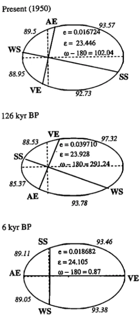
Present (1950) 88.9 S
VE
126 kyr BP VE 88.53 85.37 AE 93.78 6 kyr BP SS 93.46AE
VE
89. WS •93.38Figure 1. Earth's orbital elements for present, 126 kyr B.P., and 6 kyr B.P., where e is the eccentricity, e is the obliquity, and to is the longitude of the perihelion.
insolation values computed for the same astronomical posi- tions, i.e., the same angular position, along the Earth's orbit
relative to equinoxes and solstices. Indeed, comparing insola-
tion curves for the same dates will be misleading. Even if we
assign the same date to the vernal equinoxes of two different
periods, then their autumnal equinox and solstices will auto-
matically occur at a different date due to the change in the length of the seasons.
When considering paleoclimate simulations performed with
an AGCM, different procedures have been followed. For ex-
ample, for simulations of the 9 kyr B.P. climate, Kutzbach and
Otto-Bliesner [1982] have accounted for the change in the
length of the seasons, whereas Mitchell et al. [1988] have kept
seasons similar to present day. These two simulations have also
used a different reference date to define the "calendar" (i.e.,
assignment of a date to each day) at 9 kyr B.P.: Kutzbach and
Otto-Bliesner [1982] have fixed the 9 kyr B.P. vernal equinox at
March 21, and Mitchell et al. [1988] have fixed the 9 kyr B.P. summer solstice at June 22. Thus both the 9 kyr insolation
changes and the 9 kyr B.P. minus present monthly mean dif-
ferences cannot be directly compared between these two sets
of simulations.
To date, no study of the impact of such choices of calendar
and definition of seasons has ever been published. However,
Loutre [1993] has shown significant differences when cornpar-
ing insolation computed for two different periods either using
the same astronomical portion or the same date. In the frame-
work of PMIP, where model-model comparisons for past cli-
mate will be conducted, differences in the procedure used may
not be negligible and need to be quantified.
In the following, we will discuss in details the influence of
calendar and season definitions for paleoclimate simulations.
To better emphasize the sensitivity to a change in the length of
the seasons, we have essentially analyzed results for the 126 kyr
B.P. climate for which the changes are more important than for
the 6 kyr B.P. climate.
We first describe the orbital configuration for the period of
interest. We then define two calendars to analyze the impact of
the choice of a calendar on the solar radiation differences at
the top of the atmosphere. Similar analyses are then conducted
for the climate response, using simulations performed with the
atmospheric general circulation model (AGCM) of the Labo-
ratoire de M6t6orologie Dynamique (LMD).
2. Insolation Changes and Orbital
Configuration
2.1. Defining a "Calendar" for Past Insolation
Today, Earth is at the aphelion during northern hemisphere (NH) summer, and at the perihelion during NH winter,
whereas 126,000 years before present it was the contrary (Fig-
ure 1). The eccentricity was also higher at that time. Conse-
quently, the NH summer season was shorter. Indeed, following
the Kepler's laws, the time elapsed between two positions of the Earth along the ellipse is proportional to the area covered. If h is the true longitude, i.e., the angle used to define the Earth position relative to the vernal equinox, then time and h are related by
2•r r 2 dX
•-dt = 2(
al-e2)•/2,
(1)
where r is the Earth-Sun distance, e is the eccentricity, T is the
1-year period, and a the semimajor axis of the elliptical orbit.
For example, 126 kyr B.P., the precession of the equinoxes,
together with a larger eccentricity, reduced the time between
the vernal equinox (VE) and the summer solstice (SS) by 4
days, the time between SS and the autumnal equinox (AE) by 8 days but increased the time between AE and the winter
solstice (WS) by 4 days and the time between WS and VE by
8 days (Figure 1). The differences were less 6 kyr B.P. but
reached 4 days for the SS-AE and WS-VE intervals.
Equation (1) determines the Earth movement but does not
provide any absolute reference for time along the orbit. To
compare two insolation curves, like 126 kyr B.P. and today, we
then need to phase one curve relative to the other in order to
study the impact of changes in the seasonal variations of inso-
lation. In other words, a reference date must be arbitrarily chosen if we want to define a past calendar, as is done for
climate models.
The usual solution defines the date of the vernal equinox as the reference, i.e., fix March 21 at noon to VE for any period of the past. With this choice, two different insolation patterns are in phase around the vernal equinox but cannot be in phase
around the autumnal equinox and the solstices (Figure 2)
which thus occur at a different date for the two different past periods. However, there is no reason to prefer synchronized VE to any other position along the ellipse. In particular, the
JOUSSAUME AND BRACONNOT: SEASONS FOR PALEOCLIMATE SIMULATION 1945
date of AE (or of one of the solstices) could also be chosen as
a reference. For instance, if we choose to phase the AE date for 126 kyr B.P. and today, we would end up with a curve similar to the previous one but shifted in time (Figure 2).
These two curves describe the same insolation seasonal cycle,
but compared to the present day for a given date, they lead to
different changes in insolation. Around VE and AE, where the
phase shift between the two 126 kyr B.P. curves is maximum
(12 days), the difference represents about 10% of the insola-
tion received and is as large as the difference between 126 kyr B.P. and present.
Differences induced just by different reference dates used for past calendars are, therefore, not negligible. Thus it is
crucial for model-model comparisons to use exactly the same
time reference (calendar) in all model simulations in order to
compare the same daily insolation at the top of the atmo- sphere. For PMIP it was decided to fix the VE at March 21 noon.
2.2. Classical Versus Angular Definition of Seasons
Once a calendar has been defined for past climates, how do we account for the change in the length of the seasons to
analyze model results? Two alternative procedures have been
followed by modelers which are first compared for the insola- tion patterns and then for model results (section 3).
In most cases, once a reference date has been chosen,
months or seasons are defined following the present-day cal-
endar. In this procedure, referred to as "classical" in the fol-
lowing, averages are performed over the same number of days
and for the same dates as today's, for any period of the past.
However, following (1), months or seasons do not then cover
the same portion of the Earth's orbit with respect to equinoxes
and solstices for two different orbital configurations.
As an alternative definition of seasons, it seems appropriate
to compare values of insolation for the same positions of the
Earth along its orbit with respect to the VE [Laskar et al.,
1993]. Midmonths can be defined [Berger, 1978] by dividing the
o 600 _ 500 - _ 400 -
?E
300-
200 - 100- 0 0 60 120 180 240 300 360 I I • I • I • I • I I 600 -500 _ -400 -300 -200 -100 0 120 180 240 300 360 daysFigure 2. The 60øN daily insolation at the top of the atmo- sphere for present with March 21 as the vernal equinox (VE) date (solid line), 126 kyr B.P. with the same VE date as present
(dashed line), and 126 kyr B.P. with the same autumnal equi-
nox (AE) date as present, i.e., September 23 (dotted line).
Solar radiation has been calculated with a solar constant So -
1365 W m -2 as recommended for the Paleoclimate Modeling
Intercomparison Project (PMIP).
Table 1. First Day and Length of Angular Months for 126 kyr B.P. and 6 kyr B.P. (365-day Year) With Vernal Equinox
Fixed to March 21
126 kyr B.P. 6 kyr B.P.
Day/Month Length Day/Month Length
January 25/12 34 February 28/01 31 March 28/02 32 April 01/04 30 May 01/05 29 June 30/05 27 July 26/06 28 August 24/07 28 September 21/08 28 October 18/09 32 November 20/10 32 December 21/11 34 28/12 29/01 28/02 01/04 02/05 02/06 01/07 31/07 29/08 27/09 27/10 26/11 32 3O 32 31 31 29 3O 29 29 3O 3O 32
The dates are referred to the present calendar months.
elliptical orbit in regular 30 ø increments of the true longitude,
starting from the VE. Insolation patterns are then automati- cally phased for any period of the past since equinoxes and
solstices are 90 ø apart from each other. Moreover, these pat-
terns are independent of any time reference [Suarez and Held,
1979]. As a counterpart, these midmonths cannot be assigned
the same calendar dates through time. Following this proce- dure, "angular" seasons can be defined, based on astronomy,
as angular sectors along the orbit.
For today, the two approaches are equivalent. Our present-
day Gregorian calendar, which is a lunisolar calendar, uses a
temporal definition of months and seasons that follows the
astronomical one. Indeed, if we define astronomical seasons as
90 ø sectors in longitude between equinoxes and solstices, mod-
ern NH winter seasons are shorter in time than modern NH
summer seasons, since today the Earth's orbital speed is greater at perihelion than at aphelion. This is reflected in our calendar by 30 + 28 + 30 days in January-February-March against 31 + 31 + 30 in July-August-September.
In the following, we adopt an angular definition of months, similar to that of Kutzbach and Gallimore [1988], where "an- gular" months are defined by matching beginning and ending of celestial longitudes for each period. On the basis of these longitudes the number of days in each month and the dates relative to the present calendar months can be found using (1) and setting March 21 at VE (0 ø celestial longitude). Lengths and dates of "angular" months at 126 kyr B.P. and 6 kyr B.P. are given in Table 1 for a 365-day year.
2.3. Season Definition and Insolation Changes
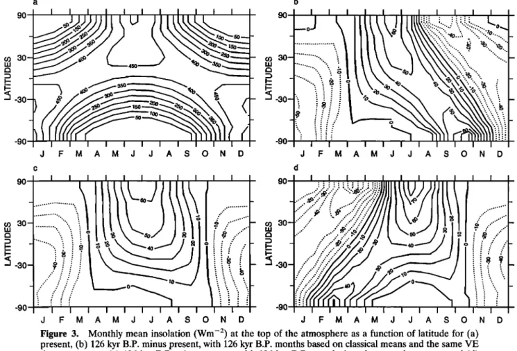
Using the "classical" and the "angular" definitions of months defined above, we can display the insolation changes between 126 kyr B.P. and today as a function of both time and latitude (Figure 3).
Let us consider first Figure 3b where "classical" months are
used and where we assume the same reference date for both
the 126 kyr B.P. and the present VE (Figure 3a). As expected
by the increase of eccentricity and the precession of the equi-
noxes, NH midlatitudes received about 40 to 50 W m -2 more
energy during summer 126 kyr B.P. than today. The patterns of differences exhibit a large structure in autumn with a north- south orientation, indicating a solar radiation reduction of
30
L
-30
-90 I I I I I I I I I I I J F M A M J J A S O N D c 30--:30-
-90 d I I I I I I I I I I I / 90 I ..!.-.[...I ... I I I I I II I' -30 ....'"
-90 I I I J F M A M J J A S O N D J F M A M J J A S O N DFigure 3. Monthly
mean
insolation
(Wm
-2) at the top of the atmosphere
as a function
of latitude
for (a)
present, (b) 126 kyr B.P. minus present, with 126 kyr B.P. months based on classical means and the same VE
date as present, (c) 126 kyr B.P. minus present, with 126 kyr B.P. months based on angular means, and (d)
same as Figure 3b but with the same AE date as present.
September
and an increase
of about
60 W m -2 at high south-
ern latitudes in October.
The "classical" definition of months being dependent on a
reference date, we could have as well chosen to fix the autum-
nal equinox (AE) as a reference date (September 23 as for
today). Although NH summers still receive more energy, the
north-south orientation in autumn totally disappears and is
replaced by a south-north orientation in spring (Figure 3d).
These patterns are strongly dependent on the choice of time
reference and simply reflect that 126 kyr ago the astronomical
summer season was shorter. Indeed, when the date of the VE
is imposed to be the same as today at 126 kyr B.P., the 126 kyr
B.P. AE occurs on September 11. With this choice of reference
date, the 126 kyr B.P. autumn begins earlier than today: inso-
lation is consequently weaker in the NH and stronger in the
SH, inducing a north-south pattern in Figure 3b. What is then
called September at 126 kyr B.P. (September 1-30) is shifted
by 12 days toward winter relative to the present-day orbital
configuration, i.e., represents a mixture of present-day Septem-
ber and October with respect to the Sun declination. Similarly,
the same analysis performed with a calendar reference date
fixed at the AE leads to the conclusion that the 126 kyr B.P.
spring began later (Figure 3d). The contradiction between the
two figures (Figures 3b and 3d) then only results from an arbitrary choice of calendar, but there is no way to decide which one is right.
To avoid the arbitrary choice of reference date, let us con- sider the "angular" definition of months (Figure 3c). With this
definition the large shifts found in autumn (Figure 3b) or
spring (Figure 3d) totally disappear. Insolation values for the
same astronomical positions are directly compared for two different climatic periods. No more phase lags or leads bias the insolation change patterns.
It is noteworthy that the differences between the "classical"
or "angular" approaches, or even between two arbitrary
choices of reference date for the "classical" months, can be as
large as 40 W m -2, i.e., as large as the Milankovitch forcing we
are considering. As seen in the next section, this feature, also
found for 6 kyr B.P. (not shown), just emphasizes that the
Milankovitch forcing remains weak compared to the very
strong seasonal variations of insolation.
2.4. Respective Impact of the Phase and Length of the "Monthly" Averages
However, none of the above ways to estimate monthly
means is entirely satisfactory. With classical means, insolation
patterns are not in phase and experience large differences
according to the arbitrary calendar reference. Angular means
seem more appropriate to analyze seasonal insolation differ-
ences, but the differences are performed between months that
do not incorporate the same number of days. We can then wonder whether the change in the number of days introduced in the "angular" months does not produce a similar bias as the
phase shifts associated with the classical means.
To answer this question and to emphasize which method is
JOUSSAUME AND BRACONNOT: SEASONS FOR PALEOCLIMATE SIMULATION 1947 90 I I I I I I I ! I I I 60- - 30- - i • 0- - J F M A M J J A S O N D
Figure 4. Mean root-mean-square
errors
(in 10
-] W m -2) as defined
in equation
(3) in the estimation
of
monthly mean insolation as a function of time and latitude when (a) a phase shift ranging from -4 to +4 days
is introduced for each month and (b) the length of the month is decreased or increased symmetrically from
-4 to +4 days.
modification of the length of the months. We base our analyses
on monthly average insolation computed for a present 365-day
year.
To estimate the impact of a phase shift, we compute monthly mean insolations shifted by -4 to +4 days relative to the reference but including the same number of days. In that case,
if N represents the number of days in the month, xi the daily
values of insolation, and at the number of days by which the mean is shifted from the reference, the perturbed monthly
mean for a given at is
I dayN+ 8t
•'(
at)
---
•[ • Xi,
(2)
i= dayl +
where day 1 and day N are the first and the last days, respec-
tively, of a "classical" month. For at varying between -4 and
+4 days, the mean root-mean-square error is then
e = sqrt •
(X-(atj)
-5-)
2 ,
j=l
(3)
with X- = X'(0). Computed for each month and each latitude
(Figure 4a), this error reaches 10 W m -2 in spring and autumn.
This result is not surprising: for a phase shift at, the difference
between the perturbed mean and the reference can be approx-
imated by
(x N -- Xl )
at) -- at N
(4)
which is of the order of the derivative of the insolation curve.
The error is thus maximum at high latitudes where the ampli-
tude of the seasonal cycle is the largest and for months near the
equinoxes. The derivative can reach 90 W m -2 over 1 month.
For a 4-day shift in insolation it leads to an error of 12 W m -2.
For 126 kyr B.P., where the shift reaches 12 days, we obtain
about
36 W m -2. The phase
shift alone
can then explain
most
of the features displayed in Figures 3b (3d) in autumn (spring).
Similarly, we can estimate the impact resulting from a
change in the length of months by considering the mean root-
mean-square differences between monthly means computed with more or less days than the reference but in phase with the
reference (days are added or subtracted symmetrically). In that
case, for a given at the perturbed monthly mean is
1 dayN+
and the mean root-mean-square error for/St varying from -4 a0 to +4 days is also given by (3). This error (Figure 4b) is of the
order of 1 to 2 W m -2 at high latitudes and is smaller than the
previous ones by an order of magnitude. In that case, the e0-
difference between the perturbed mean and the reference can
be approximated by
AX-(/St)
= N + 2/St 2
X'
(6)o lO-
-
0•
which is small since (X N q- x•)/2 practically equals X' in most -
cases, except at high latitudes near solstices. Variations of a -10.
few days in the length of a month have nearly no impact on the
monthly mean. 12
The error done on angular means is thus a second-order
effect compared to the error introduced on classical means by 10-
phase shifts. Angular means then seem more appropriate to study insolation differences between two climates, at least
when
looking
at differences
induced
by changes
in orbital
pa-
E 6-rameters. E
3. Implications for Model Results
3.1. Numerical ExperimentsThe way monthly means are defined is very sensitive when
analyzing insolation changes. We may wonder how much it
may influence the analyses of model results. In the following,
we study the impact of monthly mean definitions on the com-
parison between 126 kyr B.P. and modern climates, as simu-
lated by the AGCM developed at the Laboratoire de Met6o-
rologie Dynamique (LMD) [Sadourny and Laval, 1984; Le
Treut and Laval, 1984].
Simulations have been performed with version 4 of the LMD
model [Le Treut and Li, 1991], using the low-resolution version
which includes 48 grid points regularly spaced in longitude, 36
points regularly spaced in sine of latitude, and 11 vertical
levels. The model includes the radiative scheme described by
Fouquart and Bonnel [1980] for solar radiation and the scheme
developed by Morcrette [1991] for infrared radiation. Conden-
sation is produced using three schemes in a sequential mode:
a moist adiabatic adjustment [Manabe and Strickler, 1964], a
Kuo-type scheme [Kuo, 1965], and supersaturation for noncon-
vective precipitation. In this version of the model the land surface scheme is quite simple [Laval et al., 1981] and com- putes soil moisture for a single 1-m-deep soil layer. Surface
albedo is prescribed from climatology [Schutz and Gates, 1972]
but is increased whenever there is snow. The model is used
with full seasonal cycle but no diurnal cycle.
In the two experiments the CO 2 level has been fixed to
preindustrial value (270 ppm), sea surface temperatures (SST)
and both sea ice temperatures and sea ice extent have been
prescribed to their modern values. The experiments only differ
by their orbital parameters, which are given in Figure 1. For both climatic periods we keep March 21 at noon as the VE reference date. The model is run with a 360-day year which
does not change the conclusions obtained in section 2. Each
simulation is a 16-year run. The mean seasonal cycle is esti-
mated by averaging the last 15 years, and the departures from
the mean seasonal cycle for each of the 15 years are used to
estimate the model internal variability and assess the statistical
significance of the results.
A full discussion of the simulations can be found in de Noblet
et al. [1996]. We therefore only recall here the main features 4•
air
temperature
//""•
Europa
a
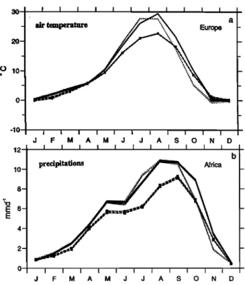
I I I I I I I I i I I F M A M J J A S O N D I I I I I I I I I I I . b precipitations ;;- Africa ...'""' • ß ' • I I I I I I I I I I I J F M A M J J A S O N D
Figure 5. (a) Simulated surface air temperature over Europe
and (b) precipitation over Africa for present (dashed line), 126
kyr B.P. using classical monthly means (dotted line), and 126
kyr B.P. using angular monthly means (solid line). Europe
corresponds to all the continental grid points from 40øN to
70øN and 10øW to 30øE. Central Africa is the region extending from 6øN to 20øN and 13øW to 45øE. Error bars represent the
95% confident interval for the mean accounting for the inter- annual variability.
characterizing the 126 kyr B.P. climate. In response to the
increased northern hemisphere seasonality of insolation at 126
kyr B.P., surface air temperature was 3 ø to 7øC warmer over most of Eurasia. The land/sea contrast was therefore en-
hanced, and the monsoon flow penetrated farther inland. Pre-
cipitation was increased over northern India, southern Tibet,
and western China, exceeding present-day values by 4 to 5 mm
d -•, and was decreased over the southern tips of India, In-
dochina, and in southeastern Asia. A similar intensification
was simulated in equatorial Africa with increased precipitation
over the Sahel and southern Sahara.
3.2. Discussion of Model Results
In this paper, we only focus on the impact of season defini-
tion on the analyses of the differences between the two cli- mates. We have thus performed the monthly means at 126 kyr
B.P. using the classical and the angular definition of months, as
defined in section 2 (for a 360-day year, see appendix). Fol-
lowing these definitions, monthly averages of surface air tem-
perature over Europe (10øW-30øE; 40øN-70øN) and of precip-
itation over central Africa (13øW-45øE; 6øN-20øN) are plotted
as a function of month in Figure 5 for 126 kyr B.P., and are
compared to the present-day results. The error bars represent
the 95% confidence interval accounting for the model interan-
nual variability. Note that when classical monthly means are
used at 126 kyr B.P., the months in Figure 5 have the same
JOUSSAUME AND BRACONNOT: SEASONS FOR PALEOCLIMATE SIMULATION 1949 0.0 M•x: 5.73 MIn: -a.14 -90 i -180 -150 -120 -90 -60 -30 0 30 LONGITUDE I I I 60 90 120 150 180 ..4• .... o • 2. o •.o b
•.o .... •i•!':•i •i•::•!•,•.:. ..-.-.-../ .'•.'"•' •.. ".•. '..'•::•: '•,. •.•., ... ..:... •'
00
••
>..
oo
,
-180 -150 -1• -• -• -30 0 • • • 1• 150 180 LONGITUDE Max ß 12.70 MIn -8 92I(,.,}i!•
-
2.0
C
60 - '0 "::i:!•i i•i•:. i :::!•:i:• i ' ' ,. --
o-_?
-
oo
_
-30 - [0 - •0'0•
•
-•__
.•, ••_ •, ,:
.... • - -.,•.
/
I',
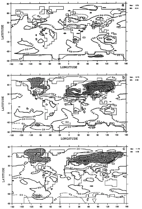
'•/ , • Xr • 'T/I I , -180 -150 -1• -• -60 -30 0 • • • 1• 150 180 Max, 11 78 MInFigure 6. September
air temperature
differences
between
(a) 126 kyr B.P. classical
means
and present,
(b)
126 kyr B.P. angular means and present, and (c) 126 kyr B.P. angular means and 126 kyr B.P. classical means.
Isolines at every 2øC.
Earth's orbit relative to equinoxes and solstices. On the other
hand, when angular monthly means are considered on the
same figure, the 126 kyr B.P. months have the same longitudes
relative to equinoxes and solstices as today but not the same
calendar dates. Thus the two 126 kyr B.P. curves describe the
evolution of surface air temperature and precipitation as a
function of the period in the year rather than as a strict func-
tion of time.
For both definitions of monthly means, similar features are
observed. Changes in the orbital parameters at 126 kyr B.P.
produce large climatic changes, with a temperature increase of
about
5øC
over Europe
in summer
and about
6 mm d-• more
precipitation over Africa. However, as for the insolation pat-
terns (Figure 3), the major differences between the two season
definitions are displayed in autumn. As can be inferred from
the error bars, they are statistically significant and even as large
as the differences between 126 kyr B.P. and present. This is due
-90 -180
==
-
-150 -120 -90 -60 -30 0 30 60 LONGITUDE 90 120 150 180 Max 1520 MIn ß -467 _ ... : .... .% 0 •- •O••
0-
-
.• _ 0.0 '• •.":'• • :'-- -'>;" "'"'"" .i -• +:.:.:.',--., ... '. • '. ß • -1• -150 -1• -• -• -• 0 • • • 1• 1• 1• LONGITUDE1.0
I
I
I
I
I
I
I
I
I
I
I
1.0
C EOF 1 0.5- -0.5 0.0- -0.0 ... ß ... • ... -0.5- --0.5-1.0
I
I
I
I
I
I
I
I
I
I
I
-1.0
J F M A M J J A S O N DFigure 7. First component of the empirical orthogonal function (EOF) analysis of the surface air temper-
ature
difference
between
126 •r B.P. and present.
Principal
component
of the difference
(in relatNe
units)
with (a) 126 •r B.P. classical
monthly
means
and (b) 126 •r B.P. angular
monthly
means.
(c) Basic
vector
of the difference
with 126
•r B.P.
monthly
means
defined
as classical
means
(dotted
line) and 126
•r monthly
means defined as angular means (solid line).
and of a shorter summer season at 126 kyr B.P. With our
definitions, 126 kyr B.P. seasonal curve using classical mean
leads the present one in autumn by about 13 days. Therefore
the climatic variable autumnal averages at 126 kyr B.P. are
biased toward the NH winter season: temperatures are already
colder over Europe (Figure 5a) and precipitation weaker over
Africa (Figure 5b). With any other time reference chosen
along the orbit, the 126 kyr B.P. classical mean curve would just
be shifted relative to the control experiment, and phase leads
or lags would occur somewhere else in the year. On the other
hand, the 126 kyr B.P. angular mean curve and the present one
are in phase relative to insolation, and in autumn the 126 kyr
B.P. temperatures are still warmer than today over Europe,
JOUSSAUME AND BRACONNOT: SEASONS FOR PALEOCLIMATE SIMULATION 1951
-'80 -150 -120 -90 -60 -30 0 30 60 90 120 150 180 LONGITUDE
b
•*•*•:•*•.'.':•i.':i•i•-:.:::•.i•ii::i}ii•!i•i•::?:•iiii•i•';: •'<:• ... '•'•4!!::::!::i:•::•ili•iil ... '•'•' ... ' ":::..<-.'•.-<.•i• •'-'.:.•.•..':*•::.•:.'::;:•.->..•.-•.•;•:•.,'.• •.•'•i•-;.'•.•:;:•.•:.•r,•,•:•
I ß •::.4:;•::.•:::•:::•:::i:i:;.r', .-r• ... ___, •:!•'?•:?:t'":x.• ... -•:•-L---..x• • '""•'-' x
':'_-_-
:_:•_•--'
,
,
,,,-:',_
•_-.' ,
,
,
,
,
,
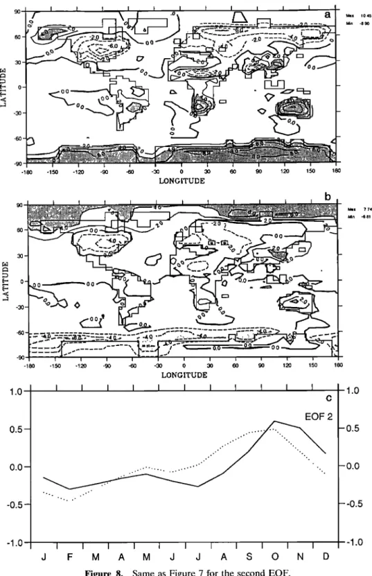
-90 -180 -150 -120 -90 -60 -30 0 30 60 90 120 150 LONGITUDE 1.0 0.5-- 0.0-- -1.0' J EOF 2 F M A M J J A S O N DFigure 8. Same as Figure 7 for the second EOF.
Max 1045 I•n -8 90 _ Max 7 74 Mn -6 81 1.0 -0.5 -0.0 -1.0
means emphasizes changes that occur within seasons defined
by the solar forcing, regardless of any reference date, such as
the VE.
Such differences between the two methods are not just local.
For example, let us consider September (Figure 6) when the
differences between the two ways of analyzing the results are
maximum due to the phasing of the VE. The surface air tem-
perature differences displayed over Europe (Figure 5) extend
over much of the NH continents (Figure 6c). They reach a
maximum over eastern Asia and North America, with more
than 10øC (Figure 6c), largely exceeding the differences be-
tween 126 kyr B.P. and today. Differences in these two areas are larger than the model internal variability and are statisti-
cally significant, as confirmed by a student ! test (not shown).
3.3. Space and Time Patterns Associated
With Each Season Definition
To better emphasize how the seasonal cycle is affected by the
onal functions (EOFs) of the differences of surface air tem- perature between the 126 kyr B.P. seasonal cycle and the
present one. EOFs have been computed for both definition of
months for 126 kyr B.P.: the classical definition of months
(Figures 7a and 8a), or the angular definition of months (Fig-
ures 7b and 8b). Time series are normalized and represent the
basic vectors (Figures 7c and 8c); spatial fields are the empir-
ical functions (in relative units). EOFs obtained with the two
definitions of monthly means for 126 kyr P.B. are superim-
posed over the same figure to better contrast the results.
The first EOF (Figure 7) accounts for nearly the same
amount of total variance for the two methods, with 58% and
60% for the classical and angular means, respectively. Their
spatial fields are roughly similar and both exhibit the same warming pattern over most areas at 126 kyr B.P., except over
Antarctica. Considering the temporal signal (Figure 7c), these
warming patterns mainly correspond to an increased seasonal
contrast in the NH and a decreased one in the SH, as expected
from the precessional effect. Figure 7c also exhibits a strong
phase shift in time. As already seen on Figure 5, the classical and angular means strongly differ in autumn.
The second EOF still accounts for a large amount of the total variance, 23% for 126 kyr B.P. using classical means minus present and 15% for the 126 kyr B.P. angular means minus present. However, both the EOF and the principal com-
ponent differ (Figure 8). For classical means, a positive peak
occurs in autumn when the first EOF reverses sign (Figure 8c).
It corresponds to a cooling over the NH continents and a
warming over Antarctica (Figure 8a). This pattern follows the
strong negative/positive pattern exhibited from north to south
for insolation arising from phase shifts due to a reduced length of the NH summer season and the particular choice of VE
reference date (Figure 3b). Therefore as much as one fourth of
the signal seems to be needed to represent a phase shift re- sulting from an arbitrary choice of calendar reference.
Since angular means do not introduce such a bias, the sec- ond component of the seasonal change, when 126 kyr B.P.
cycle is computed using angular means, exhibits a very different
pattern (Figure 8b). It emphasizes a response of high latitudes
with a positive peak in late autumn (Figure 8c). Such a pattern
corresponds to warmer surface air temperatures over the Arc-
tic sea ice and colder ones over Antarctic sea ice in October-
November. However, most of this feature is attributable to the
calendar hidden under our surface boundary conditions, as is
discussed in section 4.
4. Constraint Associated With Surface
Boundary Conditions
4.1. Surface Boundary Conditions and Calendar
Indeed, an atmospheric model is not only forced by solar
radiation incoming at the top of the atmosphere but also by
prescribed surface boundary conditions such as SST. In our
simulations the seasonal cycle of SST at 126 kyr B.P. has been
fixed following the present-day cycle, keeping track of the
present-day calendar in the 126 kyr B.P. simulations. With
respect to boundary conditions, "classical" months appear then
to be more appropriate than "angular" months. Indeed, when calculating angular means, we introduce an artificial phase shift between 126 kyr B.P. and modern surface boundary con- ditions. However, the seasonal cycle of SST has a relatively weak amplitude, due to the high ocean thermal capacity, and
differences in SST monthly means computed using either the
classical or the angular definition of months do not exceed iøC
(see Figure 9 for June and September).
In the simulations described in section 3, this constraint was
particularly strong. We have performed the simulations with a
version of the LMD AGCM that prescribes not only SST but
also sea ice temperature. The seasonal cycle of sea ice tem-
perature is much stronger than for SST and is therefore more
sensitive to the definition of months. In June, differences reach
4øC in a few places around Antarctica, when the angular mean
is slightly biased toward NH winter (Table 1). The maximum
differences occur in September when the phase shift is largest.
For that month, differences are negative in the southern hemi-
sphere and positive in the northern hemisphere, since angular
means are shifted toward NH summer. Such features are sim-
ilar to the patterns found in high latitudes for the second EOF
of angular means (Figure 8b). Figure 9 clearly shows that the
calendar hidden under our boundary conditions bias the use of
angular means.
4.2. New Set of Experiments
In order to determine which amount of the second EOF
variance is to be attributed to the inconsistency between the
astronomical seasons and the calendar hidden behind our
boundary conditions, we have performed a new set of experi-
ments, a control and a 126 kyr B.P. simulation, using a modi-
fied version of the LMD model. This version differs from the
previous one (section 3) by including a simple model of sea ice.
Sea ice extent is prescribed, but a prognostic equation has been
introduced for the sea ice temperature, accounting for the
surface energy fluxes exchanged with the atmosphere and heat
conduction through a 3-m-thick ice core. Except at high lati-
tudes over sea ice, the main features of the 126 kyr B.P. climate are very similar to the one presented in section 3. This allows
us to conclude that the bias associated with the prescribed
temperature over sea ice remains small. EOFs have also been
applied to the new set of simulations for both definitions of
months.
For the 126 kyr B.P. classical means, similar results to Figure
7a and 8a are obtained (not shown), with respective variances
of 52% and 27% for the first and second components. For the
126 kyr angular means, however, the first EOF remains similar to Figure 7b (not shown), but the large latitudinal structures
previously found at high latitudes for the second EOF (Figure
8b) completely disappear (Figure 10). This result confirms how
much our previous angular mean analyses were biased by the
sea ice temperature calendar (Figure 8b). The first EOF now
represents 69% of the total variance and the second one is
reduced to only 9%, being difficult to distinguish from the third
one (7%). It is now clear that angular means better capture the
main changes of the seasonal cycle due to insolation changes.
By using two versions of the LMD model we were also able to
emphasize the importance of the calendar associated to
boundary conditions.
We may argue that a hidden calendar still remains behind
our fixed daily sea surface temperatures. To account for the
change in the length of the seasons, one possible solution could
be to redo a daily interpolation of SSTs by assigning the
present-day monthly means to the 126 kyr B.P. angular
monthly means, i.e., by performing an interpolation accounting
for the modified lengths of months. However, the remainder
bias on the SST seasonal cycle at 126 kyr B.P. is an order of
JOUSSAUME AND BRACONNOT: SEASONS FOR PALEOCLIMATE SIMULATION 1953 '•) I I I I I I t ' I " I " I -' 80 -150 -120 -9O -60 -30 0 30 60 90 120 150 180
b
9o ....• ... I ... • ... I .... I ... ! ... JL ... [ ... •. ,,•. ... ... ;;:"-::'•"•" ... - ... f 0"•
...
;'"";"
I ' • l'ø
-
• ...
. ....
M,:
.e.•
• .
'
-180 -150 -120 -90 -60 -30 0 30 60 90 120 150 180 LONG[?UDEFigure 9. Differences of the monthly mean prescribed surface temperatures (sea ice and sea surface tem-
perature) between the ]26 kyr B.P. angular months and the present months for (a) June and (b) September.
Isolines at every ]øC.
tures (Figure 9). Moreover, this procedure would never ensure
that the resulting modified seasonal cycle would be entirely
consistent with the simulated period. The only way to avoid
such biases in the boundary conditions is to use a slab ocean,
or a coupled atmosphere-ocean model, which calculates its
own SSTs as a function of the surface energy budget. In this
case, no more hidden calendar remains and angular means
seem even more appropriate to account for insolation changes.
901 2.0 I I I I , I I I I
¬
-..--7.,.o
[ [ [ I Max ß 8 24 Mn' -4 44 30 o 0.0' ø'/"'•
0'
0
. 0
0.0 ! I I I I I -180 -150 -120 -90 -60 -30 0 30 60 90 LONGITUDE 120 150 180Figure 10. Second EOF of the difference of surface air temperature between the 126 kyr B.P. angular
monthly means and the present ones for the second set of simulations using a modified version of the
Laboratoire de Metdorologie Dynamique atmospheric general circulation model, including a simple sea ice
60- -30 - -90 -180
•
o
o
o.
ø
o•
.
_
_
n ,
-150 -120 -9O -6O -30 0 30 60 90 120 150 180 LONGITUDE Max ' 3 52 Min. -3.1560 I
";•:i•:•;•:•.i•i!i:•:
...
'' •.•':.
'"
":'
30 0 0 '::•' "-60
I I I I.••
-180 -150 -1• -• -• -• 0 • • • 1• 150 LONGITUDE Max: a.O• Mn: -3.236o
o0I•)
• 0 -30 -60 -9O -180 i i -150 -120 -9O -6o -30 0 30Max:
2.7g
Min. -1.42. I-! I 120 150 180Figure 11. September surface air temperature differences between (a) 6 kyr B.P. with classical means and
present,
(b) 6 kyr B.P. with angular
means
and present,
and (c) 6 kyr B.P. with angular
means
and 6 kyr B.P.
with classical means. Isolines at every 2øC.
5. Conclusions
When modeling past climates, we need to address the ques-
tion of defining a calendar for past periods. Indeed, because of
precessional effects amplified by eccentricity changes, the
length of seasons evolves through time. At least, when com-
paring two model simulations for past climates, the same ref-
erence date must be used in order to avoid biases in the phase
relationship between the two model simulations.
Such biases may also be introduced artificially when com-
paring model results for two different climatic periods. In that
case, no absolute phasing is possible due to changes in the
length of the seasons. Any choice of calendar, or reference
date to phase the two insolation curves, is arbitrary, and clas-
sical means arbitrarily depend on this reference date. The only
way to avoid biases in the analyses due to phase lags or leads
JOUSSAUME AND BRACONNOT: SEASONS FOR PALEOCLIMATE SIMULATION 1955
astronomical positions or angular positions along the elliptical
orbits. Such a definition of seasons is physically based and
allows to better analyze the response of climate to changes in
insolation forcing. As demonstrated here, the use of one or the
other approach has implications on the quantification of the
changes between two periods. The main changes in the
seasonal cycle appear in both season definitions, "classical" or
"angular," but differences can appear for some seasons that
may bias and even change the interpretation of model
results.
Although already stated by several authors, differences be-
tween the various possible procedures had, until now, not been
quantified. Our analyses show that such differences cannot be
neglected. It also suggests that when reporting paleoclimate
simulation results, it is necessary to specify not only the calen-
dar reference but also which definition of months has been
chosen for model analyses. Similar conclusion were also ob-
tained for 6 kyr B.P. experiments, as illustrated in Figure 11
from changes in September surface air temperatures. How-
ever, the amplitude is weaker because the changes in the
length of the seasons at 6 kyr B.P. lead at most to a shift of 5
days compared with the present.
Using months based on astronomical longitudes may also be
of interest for the present-day orbital configuration when com-
paring models using a 365-day year and models using a 360-day
year. Indeed, the same type of problem arises when we want to
define a calendar for a 360-day year simulation. With the LMD
model used in this paper, the VE date is fixed at March 21 and
30-day-long months are then defined. Such months then can-
not keep the same phase for insolation relative to monthly means based on a 365-day year. Differences between the two
insolation curves (not shown) can reach 5 to 8 W m -2 at high
latitudes, as a result of shifts of a few days. Such biases were
already discussed by Slingo [1982] who shifted the 360-day year
date of the perihelion by 1 day to minimize the differences with
a 365-day year. Using angular means for the 360-day year, i.e., defined on the same longitude values as for the 365-day year, completely erase such differences.
However, using angular or classical seasons does not solve
all the questions addressed by model analyses. Some phenom-
enon may require more detailed analyses through time series,
such as the 30- to 60-day oscillation. Statistical analyses of
temporal series would have to be done separately for the two
climatic periods. Both the impossibility to phase two insolation
curves and the chaotic nature of the atmospheric circulation
would cancel the possibility to produce day-by-day differences.
We have shown a strong sensitivity of the changes of climatic
variables according to the procedure used to define seasonal or
monthly means. We may then wonder which procedure is more
adequate to compare model results to proxy data. The choice
may depend on the type of proxy data. Our feeling is that in most cases, plants or living species will be sensitive to the seasonal cycle of insolation, i.e., astronomical positions, in
agreement with the use of angular months. However, we would
like to leave this question open for discussion among paleocli-
matologists.
Appendix: Angular Means for a 360-day Year
The LMD model uses a 360-day year. Then, angular monthly
means are defined in Table A1 as follows:
Table A1. First Day and Length of Angular Month for 126 kyr B.P. and 6 kyr B.P. for a 360-day Year
126 kyr B.P. 6 kyr B.P.
Day/Month Length Day/Month Length
January 24/12 33 27/12 31 February 27/01 33 28/01 32 March 30/02 31 30/02 31 April 01/04 30 01/04 31 May 01/05 28 02/05 30 June 29/05 27 02/06 29 July 26/06 27 01/07 29 August 23/07 27 30/07 28 September 20/08 29 28/08 29 October 19/09 30 27/09 29 November 19/10 32 26/10 30 December 21/11 33 26/11 31
The dates are referred to the present-day calendar with 30-day
months.
Acknowledgments. We particularly thank K. E. Taylor for many controversial but very stimulating discussions about insolation. We also acknowledge A. Berger and M. F. Loutre for helpful comments on
astronomical seasons. We thank N. de Noblet and G. Ramstein for
their participation in the model simulations as well as J. Y. Peter- schmitt for his useful improvement of the graphic package. We thank the Laboratoire de Mdtdorologie Dynamique for providing us their AGCM. This work was supported by an EEC contract EV5V-CT94- 0457 and computing time provided by the Commissariat h l'Energie Atomique.
References
Berger, A., Long-term variations of daily insolation and Quaternary climatic changes, J. Atmos. Sci., 35, 2362-2367, 1978.
Berger, A., Milankovitch theory and climate, Rev. Geophys., 26, 624-
657, 1988.
Berger, A., and M. F. Loutre, Insolation values for the climate of the
last 10 million years, Quat. Sci. Rev., •0(4), 297-317, 1991.
Berger, A., and M. F. Loutre, Precession, eccentricity, obliquity, inso- lation and paleoclimates, NA TO ASI Set., Long-Term Climatic Vari- ations, •(22), 107-145, 1994.
de Noblet N., P. Braconnot, S. Joussaume, and V. Masson, Sensitivity of summer monsoon regimes to orbitally induced variations in in- solation 126000, 115000 and 6000 years before present, Clim. Dyn.,
12, 598-603, 1996.
Fouquart, Y., and B. Bonnel, Computations of solar heating of the Earth's atmosphere: A new parameterization, Beitr. Phys. Atmos., 53,
35-62, 1980.
Gallimore, R. G., and J. E. Kutzbach, Snow cover and sea ice sensi-
tivity to generic changes in Earth orbital parameters, J. Geophys.
Res., 100, 1103-1130, 1995.
Imbrie, J., et al., On the structure and origin of major glaciation cycles, 1, Linear responses to Milankovitch Forcing, Paleoceanography, 7,
701-738, 1992.
Joussaume, S., and K. Taylor, Status of the paleoclimate modeling
intercomparison project (PMIP), in Proceedings of the First Interna-
tional AMIP Scientific Conference, WCRP-92, WMO/TD-732, pp. 425-430, World Meteorol. Organ., Geneva, 1995.
Kuo, H. L., On the formation and intensification of tropical cyclones through latent heat release by cumulus convection, J. Atmos. Sci., 22,
40-63, 1965.
Kutzbach, J. E., and R. G. Gallimore, Sensitivity of a coupled atmo- sphere/mixed layer ocean model to changes in orbital forcing at 9000 years B.P., J. Geophys. Res., 93, 803-821, 1988.
Kutzbach, J. E., and B. L. Otto-Bliesner, The sensitivity of the African- Asian monsoon climate to orbital parameter changes for 9000 years B.P. in a low-resolution general circulation model, J. Atmos. Sci., 39,
1177-1188, 1982.
Kutzbach, J. E., and F. A. Street-Perrot, Milankovitch forcing of fluc- tuations in the level of tropical lakes from 18 to 0 kyr BP, Nature,
Laskar, J., F. Joutel, and F. Boudin, Orbital, precessional, and insola-
tion quantities for the Earth from -20 Myr to + 10 Myr, Astron. Astrophys., 270, 522-533, 1993.
Laval, K., R. Sadourny, and V. Serafini, Land surface processes in a
simplified GCM, Geophys. Astrophys. Fluid Dyn., 17, 129-150, 1981.
Le Treut, H., and K. Laval, The importance of cloud-radiation inter- action for the simulation of climate, in New Perspectives in Climate Modelling, edited by A. Berger and C. Nicolis, Dev. in Atmos. Sci., 16,
199-221, 1984.
Le Treut, H., and Z. X. Li, Sensitivity of an atmospheric general circulation model to prescribed SST changes: Feedback effect asso-
ciated with the simulation of the cloud optical properties, Clim.
Dyn., 5, 175-187, 1991.
Manabe, S., and R. F. Strickleer, Thermal equilibrium in the atmo-
sphere with a convective adjustment, J. Atmos. Sci., 21, 361-385, 1964.
Milankovitch, M., Thdorie mathdmatique des phdnomenes thermiques produits par la radiation solaire, Gauthier-Villars, Paris, 1920.
Loutre, M. F., Parametres orbitaux et cycles diurnes et saisonniers des
insolations, Ph.D. thesis, Fac. des Sci., Univ. Cath. de Louvain, Louvain-la-Neuve, France, 1993.
Mitchell, J. F. B., N. S. Grahame, and N. K. J., Climate simulations for
9000 years before present: Seasonal variations and effects of the Laurentide ice sheet, J. Geophys. Res., 93, 8283-8303, 1988. Morcrette, J. J., Radiation and cloud radiative properties in the EC-
MWF operational weather forecast model, J. Geophys. Res., 96,
9121-9132, 1991.
Phillipps, P. J., and I. M. Held, The response to orbital perturbations
in an atmospheric model coupled to a slab ocean, J. Clim., 7, 767-
782, 1994.
Rind, D., D. Pettet, and G. Kukla, Can Milankovitch orbital variations
initiate the growth of ice sheets in a general circulation model?, J. Geophys. Res., 94, 12,851-12,871, 1989.
Royer, J. F., M. Ddqud, and P. Pestiaux, A sensitivity experiment to
astronomical forcing with a spectral GCM: Simulation of the annual cycle at 125 000 and 115 000 BP, in Milankovitch and Climate, part 2,
edited by A. L. Berger et al., pp. 733-763, 1984.
Sadourny, R., and K. Laval, January and July performance of the LMD general circulation model, New Perspectives in Climate Modelling,
edited by A. Berger and C. Nicolis, Dev. in Atmos. Sci., 16, 173-198,
1984.
Schutz, C., and W. L. Gates, Global climatic data for surface, 800 mb, 400 mb, Tech. Rep. 1029, Rand Corp., ARPA, Santa Monica, Calif.,
1972.
Slingo, A., Insolation calculation for a 360-day year, Meteorol. 0 20
Tech. Note, Meteorol. Office, Bracknell, England, 1982.
Suarez, M. J., and I. M. Held, The sensitivity of an energy balance climate model to variations in the orbital parameters, J. Geophys.
Res., 84, 4825-4836, 1979.
P. Braconnot and S. Joussaume, LMCE, DSM, Orme des Merisiers,
Bit 709, CE Saclay, 91191 Gif-sur-Yvette, Cedex France. (e-mail:
syljous@lmce.saclay.cea.fr)
(Received September 2, 1995; revised May 10, 1996;
![Figure 4. Mean root-mean-square errors (in 10 -] W m -2) as defined in equation (3) in the estimation of monthly mean insolation as a function of time and latitude when (a) a phase shift ranging from -4 to +4 days is introduced for each month](https://thumb-eu.123doks.com/thumbv2/123doknet/13020591.381299/6.906.225.687.93.618/figure-defined-equation-estimation-insolation-function-latitude-introduced.webp)

![Figure 9. Differences of the monthly mean prescribed surface temperatures (sea ice and sea surface tem- perature) between the ]26 kyr B.P](https://thumb-eu.123doks.com/thumbv2/123doknet/13020591.381299/12.906.181.721.100.621/figure-differences-monthly-prescribed-surface-temperatures-surface-perature.webp)