HAL Id: cea-01818751
https://hal-cea.archives-ouvertes.fr/cea-01818751
Submitted on 14 Jan 2019
HAL is a multi-disciplinary open access
archive for the deposit and dissemination of
sci-entific research documents, whether they are
pub-lished or not. The documents may come from
teaching and research institutions in France or
abroad, or from public or private research centers.
L’archive ouverte pluridisciplinaire HAL, est
destinée au dépôt et à la diffusion de documents
scientifiques de niveau recherche, publiés ou non,
émanant des établissements d’enseignement et de
recherche français ou étrangers, des laboratoires
publics ou privés.
Modelling of the effect of grain boundary diffusion on
the oxidation of Ni-Cr alloys at high temperature
Léa Bataillou, Clara Desgranges, Laure Martinelli, Daniel Monceau
To cite this version:
Léa Bataillou, Clara Desgranges, Laure Martinelli, Daniel Monceau. Modelling of the effect of grain
boundary diffusion on the oxidation of Ni-Cr alloys at high temperature. Corrosion Science, Elsevier,
2018, 136, pp.148-160. �10.1016/j.corsci.2018.03.001�. �cea-01818751�
Modelling
of the effect of grain boundary diffusion on the oxidation of Ni-Cr
alloys
at high temperature
Léa
Bataillou
a,c,⁎,
Clara Desgranges
a,b,
Laure Martinelli
a,
Daniel Monceau
caDen-Service de la Corrosion et du Comportement des Matériaux dans leur Environnement (SCCME), CEA, Université Paris-Saclay, F-91191, Gif-sur-Yvette, France bSafran-Tech, rue des jeunes bois, Châteaufort, CS 80112, 78772 Magny les hameaux, France
cCIRIMAT, Université de Toulouse, CNRS, INPT, UPS, 4 allée Emile Monso, BP 44362, 33103 Toulouse Cedex 4, France
Grain boundaries in oxide scales have a strong effect on oxidation kinetics when they act as diffusion short circuits. This study proposes a quantitative evaluation of the phenomenon by modelling. Various cases of oxide microstructure evolution are treated using both analytical and numerical resolutions. Results showed that the effect of oxide grain growth on the oxidation kinetics can be analysed considering a transitory stage for which the oxidation kinetics is not purely parabolic. Some guidelines for choosing the appropriate post-treatment method for the analysis and extrapolation of experimental oxidation kinetics are given.
1. Introduction
Parabolic constants values reported in literature for chromia forming alloys [1–13] are distributed on several orders of magnitude, these values are gathered onFig. 1. It has been shown that under O2
atmospheres, chromia grow by diffusion of spieces across the oxide scale [13,15,16] and that diffusion short-circuits, such as grain boundaries in oxide scales, have a major effect on oxidation kinetics [10,17,18].
In his review on the influence of grain boundary diffusion on high temperature oxidation, Atkinson [1] showed that the values of the ex-perimental parabolic constant (kp) published for chromia are
dis-tributed over a range of about three orders of magnitude for the same temperature. Atkinson calculated theoretical kpvalues for
polycristal-line chromia using tracer diffusion coefficient from Hagel et al. [14], and kpvalue for single cristal chromia using single cristal tracer di
ffu-sion coefficient for chromia that he determined experimentally [1]. He showed that experimental reported kpvalues were closer to theoretical
values corresponding to polycrystalline chromia than to theoretical value corresponding to single crystal chromia. These experimental and theoretical kpvalues are plotted onFig. 1. Knowing that the calculated
kpfor polycrystalline chromia can be up to six orders of magnitude
higher than the one of single crystal chromia, it was concluded that chromia growth was quantitatively affected by grain boundary diffu-sion [1]. Notice that such a dispersion of reported kpvalues can also be
explained by other phenomena such as a transitory regime caused by formation of NiO [19] or the presence of reactive elements that can slow down diffusion [10,20].
Concerning the influence of grain boundaries, several authors pro-posed oxidation models taking into account accelerated diffusion by short-circuit diffusion paths. Perrow et al. [18] proposed an analytical solution for oxidation kinetics taking into account grain boundary dif-fusion in nickel oxide scales. They used the effective diffusion coeffi-cient proposed by Hart [21], which is a weighted average between lattice and short-circuit diffusion coefficients. Hart’s law was initially established for the modelling of accelerated diffusion by dislocation. However, it can be adapted to diffusion through grain boundaries. Besides the use of Hart’s law, Perrow et al. [18] added the influence of grain size evolution via a parabolic growth law. Hussey et al. [22], who worked on iron oxides growth kinetics, followed the same hypotheses as Perrow et al. [18] and determined an instantaneous parabolic rate constant in the case of a parabolic oxide grain growth. Rhines et al. [23,24] observed cubic oxidation kinetics on NiO scales associated with a cubic grain size growth. Davies and Smeltzer [25,26] proposed an analytical treatment by means of an exponential law for the decay of short-circuit proportion over time. More recently, Hallström et al. [27] proposed a numerical approach based on thermodynamics calculations applied to chromia growth. Nevertheless, this model does not take oxide microstructure evolution into account. Other authors have con-sidered the diffusion through grain boundaries in oxide scales [28–30]
⁎Corresponding author at: Den-Service de la Corrosion et du Comportement des Matériaux dans leur Environnement (SCCME), CEA, Université Paris-Saclay, Gif-sur-Yvette, F-91191,
France.
E-mail addresses:lea.bataillou@cea.fr(L. Bataillou),clara.desgranges@safrangroup.com(C. Desgranges),laure.martinelli@cea.fr(L. Martinelli),
and even the influence of oxide microstructure on oxidation kinetics [31,32], with an experimental approach.
Some different approaches have been developed concerning oxida-tion kinetics modelling by taking into account formaoxida-tion and growth of several phases which are also steps forward the description of complex oxide microstructure. Larsson et al. [33] performed a numerical simu-lation of multiphasic iron oxide growth. Nijdam et al. [34,35] devel-oped coupled thermodynamic-kinetics oxidation model, which is able to predict the phases formed and their impact on oxidation kinetics.
In this framework, this study proposes a new quantitative estima-tion of the influence of grain boundary diffusion on oxidation kinetics. Oxidation models proposed are applied on chromia-forming alloys. The studied cases consider (1) the evolution of grain size over time, (2) a grain size gradient across the oxide scale, and (3) a combination of both. For the simplest cases (1) and (2), some new analytical solutions were found. However, for the complex cases (3), which combine grain size evolution in time and space, a numerical approach is required. The numerical EKINOX model [36–38] has been used and modified for this study in order to take into account grain boundary diffusion and mi-crostructural evolutions in the oxide scale. Chromia growth kinetics were then modelled using input data based on literature experimental data [10].
Thefirst part of this paper presents the existing oxidation kinetics models available in the literature. These models take into account both lattice and grain boundary diffusion in the oxide scale according to A-type diffusion [39] and consider homogeneous oxide grain size or simple grain size growth law. The second part is dedicated to new analytical models proposed, and to the numerical modelling using the EKINOX code. These new models are able to take into account the oxide grain size growth according to a cubic law and a grain size gradient across the oxide scale. Moreover, a numerical model is adapted in order to treat the complex case of grain size growth and grain size gradient combination.
In results section kinetics obtained using the various analytical and numerical models are presented. Firstly, these oxidation kinetics are
discussed, and then, a parametric study is carried out on the effects of the oxide grain size growth kinetics. In the discussion part, the two methods, which are usually performed for the analysis and the extra-polation of experimental oxidation kinetics, are used on calculated ki-netics and they are compared. These are referred in this work as the “parabolic law” method and the “log-log” method. Finally, the two methods are compared for long term extrapolation.
2. Literature models for oxidation kinetics and extrapolation methods
2.1. Wagner’s theory simplified
In the case of continuous oxide scale formation, Wagner proposes a model for oxide scale growth that looks at diffusion across the oxide scale as the rate-limiting step [40]. A simplified expression for the parabolic rate constant can be given assuming that the species con-centrations at metal/oxide and oxide/gas interfaces are time invariant. This assumption supposes that diffusion occurs through lattice only, that the diffusion coefficient is constant and that usual hypotheses of stationarity, electroneutrality and fluxes conservation are assumed [40]: = − + e2 k (t t) e p,L 0 02 (1) = ∼ kp,L 2ΩDLΔC (2)
2.2. Diffusion models taking into account bulk and short-circuit diffusion When the influence of diffusion along short circuits is taken into account within the global diffusion phenomenon, several limiting cases can be described. These different cases depend on the space distribution of grain size and on the values of diffusion coefficients in lattice and in short circuits [41,42]. Hence three different regimes involving grain boundary diffusion are classically considered and called A-type, B-type
Fig. 1. Arrhenius plot of experimental parabolic rate constant for Cr2O3reported in literature [2–13], and calculated by Atkinson [1] using single crystal or polycrystalline chromia
and C-type diffusion. A-type and C-type diffusion represent the two limiting cases of the more general B-type.
In the A-type diffusion model, diffusing atoms are considered to get through lattice and short circuits many times during the studied time period. Therefore, A-type diffusion is often used for long term diffusion, at high temperatures. The diffusion front then corresponds to the mean of paths taken by the diffusing atoms in lattice and short circuits. A schematic illustration of the diffusion front for A-type diffusion is pre-sented inFig. 2. The diffusion front can be addressed by an effective diffusion coefficient expressed according to Hart’s law [21]:
= − +
∼ ∼ ∼
Deff DL(1 f) D fgb (3)
The parameter f can be expressed as the fraction of short-circuit surface in the material, according to Eq.(4). In the literature, there are other expressions that take into account various grain geometries and surfacic or volumic short-circuit fraction. Eq. (4) corresponds to equiaxed grains and was used by Perrow for high temperature oxidation [18].
=
f 2 /δ g (4)
If grain boundaries are considered as diffusion short circuits, δ corresponds to the grain boundary thickness and g corresponds to the grain size.
Using the A-type diffusion model requires a condition [42]. As dif-fusing atoms are considered to go through lattice and short circuits several times during the experiment, the typical observation time for this regime must be much longer than the time needed by the atoms to move from a short circuit to another through a lattice region. In other words, the mean free path must be far superior to the short-circuit spacing:
> > ∼
D t g
2 L (5)
B-type model is effective if the free mean path is the same order of magnitude as the grain size. C-type model is effective for very short times, low temperature, or very high diffusion coefficients in short circuits. The diffusion is assumed to occur almost exclusively through the short-circuit network. The following study looks at A-type diffusion, consequently, B-type and C-type diffusions are not developed. 2.3. Simplified Wagner’s theory and effective diffusion coefficient
The effective diffusion coefficient for A regime, as given by Eq.(3), can be combined with the parabolic kinetics coming from Wagner’s theory in order to take into account the influence of short-circuit dif-fusion on oxidation kinetics. Using Eqs.(1)and(3), the oxidation ki-netics becomes: = − + e2 k (t t) e p,eff 0 02 (6) with = ∼ kp,eff 2ΩD ΔCeff (7)
and using(1),(2),(3),(4)and(7)the effective parabolic constant is expressed as follows: = ⎛ ⎝ ⎜ + ⎛ ⎝ ⎜ − ⎞ ⎠ ⎟ ⎞ ⎠ ⎟ ∼ ∼ k k δ g D D 1 2 1 p,eff p,L gb L (8)
The use of Eq.(6)requires the assumptions involved in Hart’s and Wagner’s laws, but also the hypothesis that the oxide microstructure is immobilized presenting a uniform and constant grain size. Since mi-crostructure evolutions are common, Perrow et al. [18] proposed a model that takes into account the grain growth over time.
2.4. Perrow’s model
Hence, Perrow et al. [18] proposed a more complex oxidation ki-netics model for oxide scale growth with the effective diffusion coeffi-cient calculated with Hart’s relation (3), but also taking into account the evolution of the grain boundary fraction over time, which is re-presented by a parabolic grain growth during scale growth:
= − +
g t2( ) k t( t) g
g 0 0
2
(9) All grains are supposed to be identical in size and follow the same growth kinetics. The oxidation kinetics proposed in Perrow’s work [18] contains a calculation error, the exact expression is given below:
− = + + − ∼ ∼ e e k t k δD k D g k t g 4 ( ) 2 02 p,L p,L gb g L 0 2 g 0 (10) Using the same assumptions as Perrow [18], Hussey et al. [22] proposed an expression of instantaneous growth rate given by Eq.(11). This relation illustrates the fact that the scale growth can be expressed with a parabolic rate constant that evolves over time.
= = ⎛ ⎝ ⎜ + + ⎞ ⎠ ⎟ ∼ ∼ k e e t k δD D k t g 2 d d 1 2 p,I p,L gb L g 0 2 (11) 2.5. Other laws for short-circuit density evolution
2.5.1. Cubic law
Rhines et al. [23,24] proposed a model with a grain volume pro-portional to time. If the grain volume is considered as the cube of grain size, this is equivalent to a cubic growth law applied to grain size, as expressed in Eq.(12). Rhines noticed that his experimental oxidation kinetics of Ni was in good accordance with a cubic law.
= − +
g t3( ) k t( t) g
h 0 0
3
(12) However, by using the cubic grain growth law, Rhines did not dis-play the corresponding analytical expression of oxidation kinetics. This point is developed in part II of this study.
2.5.2. Exponential law
Davies and Smeltzer [25,26] modelled the case of inward oxygen diffusion through oxide scale by assuming that the diffusion of oxygen happened through the lattice and an“array” of low resistance paths (diffusion short circuits). They assumed that the proportion of low re-sistance paths decays according to an exponential law during the oxi-dation experiment. This model is not discussed or used in this study. Since it was developed for the diffusion through a random array of dislocations, it does not seem adequate for the description of diffusion in oxide grain boundaries.
2.6. Analysis of experimental oxidation kinetics and extrapolation methods This paragraph focuses on the different methods available in the literature to interpret and extrapolate the experimental oxidation ki-netics. These methods usually enable to characterize the experimental oxidation kinetics with an analytical law, and then to extrapolate them over longer time periods.
2.6.1. Parabolic law method
One way to interpret and extrapolate experimental oxidation ki-netics curves is to assume that the diffusion phenomenon in the oxide is the main rate limiting step for oxide growth. The oxidation kinetics is thus defined as a parabolic law. However, a purely parabolic law should be applied only in specific cases with the growth of a unique type of oxide, having the same diffusion properties throughout the entire ex-periment. Most of the time, a transitory regime precedes the estab-lishment of a stationary regime. It is thus necessary to adapt the parabolic law so as to correctly describe the system. Two studies by Pieraggi and Monceau [43,44] propose several parabolic laws designed for different experimental hypotheses. The following mass gain equa-tions have been written for thermogravimetric experiments, however they can be adapted to express oxide thickness. The rate Eq.(13)and kinetic law (14) given below adequately describe oxidation kinetics purely controlled by diffusion. In this case, the initial oxide grown during the transient period (t < ti) has the same protective properties
as the oxide growing at t > ti. The apparent growth rate constant can
be determined by plotting e2orΔm2versus t.
= Δm t k Δm d d 2 p (13) − = − Δm2 Δm k t( t) i2 p i (14)
The rate Eq.(15)and kinetic law(16)given below also adequately describe oxidation kinetics purely controlled by diffusion. But in this case, the initial oxide growing during the transient period (t < ti) is
much less protective than the oxide growing at t > ti. The apparent
growth rate constant can be determined by plotting e orΔm versus t1/2.
= − Δm t k Δm Δm d d 2( ) p i (15) − = − Δm Δm k t t ( i)2 p( i) (16)
The rate Eq.(17)and the kinetic law(18)given below adequately describe a general oxidation process controlled by a diffusion step characterized by the “kp” constant and an interfacial reaction step
characterized by the“kl” constant. In this case, the protective properties
of the initial oxide are identical to those of the stable oxide. = + Δm t k Δm k d d 1 (1 l) (2 p) (17) − = − + − t t Δm Δm k Δm Δm k i 2 i2 p i l (18)
The growth rate Eq. (19) and the kinetic law (20) given below adequately describe an overall oxidation process controlled by a dif-fusion step characterized by the“kp” constant and an interfacial
reac-tion step characterized by the “kl” constant. In this case, the initial
oxide that grows during the transient period (t < ti) is much less
pro-tective than the oxide growing at t > ti. This case is the most general
one. = + − Δm t k Δm Δm k d d 1 (1 l) (2( i) p) (19) − = − + − t t Δm Δm k Δm Δm k ( ) i i 2 p i l (20)
If none of the equations above(14),(16),(18)or(20) match the entire experimental curve, it is possible to look at kpas a parameter
evolving over time rather than a constant.
This approach has been proposed by Hussey et al. [22]. They cal-culated the variation of the parabolic rate constant kpover time using
Eq.(21). Later, Atkinson [45] also concluded that the kpvalue could
change over time particularly when oxide grains grow during the ex-periment. The kpvalue determined using Eq.(21)is sometimes called
“instantaneous kp” [22,43]. However, this expression must not be used
in a general way because it corresponds to the specific case described by Eq.(13). = k Δm Δm t 2 d d p,I (21) Monceau and Pieraggi [43] have developed a method to calculate kp
value locally that is better adapted to experimental cases. It is based on the localfit of experimental data within a sliding window using the complete parabolic law. Indeed, what is interesting in Eqs.(13)–(20)is that the four rate laws(13),(15),(17),(19)have a common solution in the form of Eq.(20). This means that when the growth of an oxide scale is controlled by diffusion and reaction, even after a transient regime with different oxidation kinetics, then the complete parabolic law(20) can be used tofit the oxidation kinetics. Nevertheless, in order to obtain a goodfit, both kpand klshould be constant over thefit interval. This
last point can be verified by using the complete parabolic law(22)over a sliding time interval over all the experimental data. By using this method, it is then possible to measure the variation of kpover time and
detect the time interval for which kpis or becomes constant.
= + + t A B Δm( ) C Δm( )2 (22) with = k C 1 p (23)
Contrary to Eq.(21), Eq.(22)is compatible with the growth of a first porous, or non-continuous or fast growing transient oxide layer and a second stable and slowly growing oxide, this corresponds to the most general case. When a transitory oxidation regime occurs, the value of kp
changes at the beginning of the oxidation experiment and then stabi-lizes to a stationary value, corresponding to the stationary regime. The extrapolation procedure consists in identifying of the stationary kp
value and using the kinetic law(22)to extrapolate the mass change kinetics.
This local kpapproach differs from the instantaneous kpapproach
presented previously. Indeed, the instantaneous kpcorresponds to the
derived kinetics for time t, whereas the local kpcorresponds to afit of a
portion of the oxidation kinetics curve. 2.6.2. Log-log method
If oxidation kinetics cannot be identified at first as a parabolic or a complete parabolic kinetic law, there is another method commonly employed to describe the oxidation kinetics: the “log-log” method. Without assuming any oxidation mechanism (linear, parabolic or cubic laws), the oxidation kinetics isfitted by a power law:
− =
Δm Δm k t
( )m
i log (24)
The logarithm of the mass gain (log(Δm)) is then plotted as a function of the logarithm of time according to Eq.(25)in order to ex-tract the values of m and klogfrom a linearfit.
− = +
Δm Δm
m t m k
log( i) 1 log( ) 1 log( log) (25) The extrapolation for a longer duration is done using Eq.(24). These two methods,“parabolic law” and “log-log”, are discussed in section5of this study.
3. Modelling developments for oxidation kinetics
It has been shown here that several analytical models exist to de-scribe oxidation kinetics. Some of them take into account the influence of diffusion by short-circuit paths, and their density evolution over time. The hypotheses made in the oxide microstructure evolution are quite simple. However, complex microstructure have been observed for chromia. For example, Zurek et al. [46] observed various grain sizes
across the oxide scale from nanometric to micrometric scale, and Latu-Romain et al. [16] observed equiaxed grains of hundreds of nanometers size in chromia layer in the inner part of the oxide scale, and columnar grains of hundreds of nanometres length in the layer on the outer part of the oxide scale. In the light of these complex chromia microstructures reported in literature, it seems relevant to take into account more complex grain sizes evolutions in the oxidation kinetics models con-sidering grain size evolution with time and space. Hence, the next part proposes some new original analytical models that take into account different hypotheses on grain size evolution.
3.1. Analytical models
3.1.1. Parabolic oxide grain growth law
First, Perrow’s model [18] can be re-considered without the ap-proximationD∼L(1−f)≈∼DL. Indeed, avoiding this approximation
al-lows extending the use of this model to a wider range of parameter values. The oxidation kinetics given by Perrow(10)can be expressed without the approximation∼DL(1−f)≈∼DLand by taking into account
initial conditions (e0, t0): = ⎡ ⎣ ⎢ − + ⎛ ⎝ ⎜ − ⎞ ⎠ ⎟ + − + ⎤ ⎦ ⎥ + ∼ ∼ e k t t δ k D D k t g k t g e ( ) 4 1 ( ) 2 p,L 0 g gb L g 0 2 g 0 0 2 02 (26) Consequently, the expression of the instantaneous parabolic con-stant(11)becomes: = = ⎛ ⎝ ⎜ + + ⎛ ⎝ ⎜ − ⎞ ⎠ ⎟ ⎞ ⎠ ⎟ ∼ ∼ k e e t k δ k t g D D 2 d d 1 2 1 p,I p,L g 0 2 gb L (27)
3.1.2. Cubic oxide grain growth law
By applying the cubic grain growth law according to Eq.(12), the effective diffusion coefficient defined by Eq. (3)can be expressed as follows: ⎜ ⎟ = ⎛ ⎝ − + ⎞ ⎠ + + ∼ ∼ ∼ D D δ k t g D δ k t g 1 2 ( ) 2 ( ) eff L h 03 1/3 gb h 03 1/3 (28)
The oxidation kinetics model, assuming a cubic oxide grain growth, can thus be written as follows:
= ⎡ ⎣ ⎢ − + − + − + ⎤ ⎦ ⎥ + ∼ ∼ e k t t δ k D D k t g k t g e ( ) 3 ( 1)[( ) ( ) ] 2 p,L 0 h gb L h 03 2/3 h 0 03 2/3 02 (29) 3.1.3. Grain size gradient in the oxide scale
A grain size gradient across the oxide scale is often observed. For example, Zurek et al. [46] studied the chromia scale growth on a Ni-25Cr and observed that the microstructure of the oxide scale presented a variation of grain size across the oxide scale from about 30 nm to 1μm. Kofstad [28] studied oxidation mechanisms of chromium and also described a chromia grain size difference between the outer part and the inner part of the scale.
Facing this problem, Atkinson [50] used the largest grain size in a NiO scale, grown on pure Ni, to explain the scaling kinetics. But this approximation requires quantitative assessment. It is therefore relevant to take into account the influence of heterogeneous grain sizes in the oxide scale on oxidation kinetics.
Naumenko et al. [32] and Young et al. [47] proposed an oxidation kinetics model for alumina considering a grain size gradient that re-mains constant over time i.e. a grain size proportional to the distance to the oxide gas interface. As the distance to the oxide/gas interface in-creases over time because of the oxide growth, the global grain size also increases over time. Therefore, in this model, oxide grain size is a
function of both position in oxide scale and time. According to these works [32,47] such a model is well adapted to alumina growth de-scription. It seems also relevant to be able to uncorrelate grain size evolution over time and across oxide scale for being representative of complex microstructures.
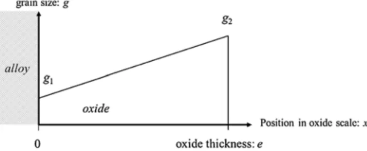
In the present work, a simple case of a uniform grain size gradient with set grain sizes at both alloy/oxide and oxide/gas interfaces is studied. The schematic illustration of the chosen grain size distribution is shown inFig. 3. The larger grain size is located at the oxide/gas interface and the smaller grain size is located at the metal/oxide in-terface, as observed by Zurek on Ni-25Cr-Mn alloys at 1000 °C in Ar-20%O2[46].
Assuming a grain size gradient across the oxide scale, the effective diffusion coefficient is expressed as follows:
= ⎛ ⎝ ⎜ − + − ⎞ ⎠ ⎟ + + − ∼ ∼ ∼ D D δ g g g D δ g g g 1 2 ( ) 2 ( ) x e x e eff L 1 2 1 gb 1 2 1 (30)
The determination of the oxidation kinetics requires the integration of Eq.(31), using Eq.(30)for the effective chemical diffusion coeffi-cient expression. = ∂ ∂ ∼ e t ΩD C x d d eff (31)
The following change of variable is done: =
y x
e (32)
With Eqs.(30)and(32), Eq.(31)becomes:
= ⎡ ⎣ ⎢ ⎛ ⎝ ⎜ − + − ⎞ ⎠ ⎟ + + − ⎤ ⎦ ⎥ ∼ ∼ e t Ω ΔC eΔy D δ g g g D δ g g g d d 1 2 ( ) 2 ( ) x e x e L 1 2 1 gb 1 2 1 (33)
By integrating Eq.(33)the following oxide scaling kinetics is ob-tained for a constant grain size gradient across the oxide scale:
= − + ⎛ ⎝ ⎞ ⎠ + + − + + + + ∼ ∼ ∼ ∼ ∼ ∼ ∼ ∼ ∼ e k (t t) e 1 δ D D log D g g δD δD D g δD δD D g 2 p,L 0 2 ( ) ( ) 2 2 2 2 02 gb L L 1 2 gb L L 2 gb L L 1 (34)
3.1.4. Combination of oxide grain size gradient and grain growth The case of grain growth with a grain size gradient across the oxide scale corresponds to a variation of grain boundary proportion in both time and space. Such a complex description of oxide scale micro-structure and evolution over time is a step further toward a more rea-listic description of chromia microstructure obtained experimentally. Moreover, the comparison of the oxide scale microstructures obtained after 3 min oxidation and 30 min oxidation indicated a growth of chromia grains over time.
This complex case of oxide microstructure evolution cannot be de-scribed with an analytical expression, it is thus treated with the nu-merical oxidation model EKINOX.
3.2. EKINOX model
EKINOX is a 1D numerical oxidation model. It has been developed to calculate chromia growth kinetics and substrate evolution during high temperature oxidation. Explicit calculations of the concentration of Ni, Cr, O, but also of metallic and oxygen vacancies in the metal/ oxide system are carried out by numerical time integration. EKINOX model can thus be useful to understand high temperature oxidation mechanisms. The metal/oxide system is divided into space elements in which fluxes and concentrations are calculated, using Fick’s laws ac-cording to afinite difference algorithm given in Eqs.(35)and(36). The set of equations that is numerically time integrated has been detailed in previous works [36–38]. The Ni-Cr version has been previously used to calculate the concentration profiles of species and vacancies in the substrate [36–38]. The present work focuses on the oxide scale growth kinetics. The oxide scale is described with two sub-lattices, the cationic sub-lattice containing chromium and chromium vacancies exclusively, and the anionic sub-lattice containing oxygen and oxygen vacancies exclusively. The predominant defects taken here into consideration for lattice diffusion in oxide scale are cationic vacancies, in agreement with experiments carried out by Tsai et al. [10]. In the present study, the effective diffusion coefficient according to Hart’s law(3)has been im-plemented instead of the pure lattice diffusion coefficient, so as to take into account the influence of grain boundaries on oxidation kinetics. This effective diffusion coefficient can vary as a function of time and across the oxide scale. Therefore, the EKINOX numerical model enables to calculate the effects of different grain growth laws and of a grain size gradient. It also allows calculating transitory oxidation regimes. Con-sequently, the next part shows how EKINOX calculations are used in order to study cases more complex than the ones previously modelled with analytical solutions. In order to validate the numerical resolution, the comparison between numerical calculations and analytical solu-tions previously mentioned is done (Fig. 4).
+ = + − − C t Δt C t J t J t e Δt ( ) ( ) ( ) ( ) Xn Xn X n 1 Xn n (35) = −∼ − + + + J ( )t D ( )t C ( )t C ( )t e e Xn eff,X n Xn 1 Xn 2 n 1 n (36) 3.3. Input data
The input data used for all EKINOX calculations presented here have been chosen in order to represent realistic physical data related to the Ni-30Cr/Cr2O3 system. Input data have been either extracted from
published literature or calculated with the Thermocalc software, using Kjellqvist model for chromia description [48]. Most oxidation para-meters come from Tsai et al. [10] who performed oxidation and dif-fusion experiments on Ni-30Cr under 1 atm of O2at 1173 K. These data
are gathered inTable 1.
For analytical calculations, input data are also gathered inTable 1 and kp,Lis determined according to the following relation:
= ∼
kp,L 2D ΔXL V (37)
With the parameters chosen for this study, kp,L= 8.10−15cm2s−1.
Relation(37)is identical to relation(2)with: =
ΔX ΔC Ω
V (38)
The input data relative to grain growth rate depend on the case studied. All input parameters used to perform the different calculations are summarized inTable 2. For information, the table also gives the corresponding grain size in the oxide at the end of the simulation (300 h oxidation). Cases #P1, #P2, #C1, #C3 lead to unrealisticfinal grain sizes. These calculations have been performed for a parametric study in order to understand the influence of grain growth on the oxidation kinetics.
For each case, the effective diffusion coefficient is calculated by combining Eqs.(3),(4)and(9)or(12). The effective diffusion coeffi-cients for each case are plotted inFigs. 5–7. When the grain growth is fast, both the proportion of short-circuit diffusion and the effective diffusion coefficient decrease rapidly. As a result, the faster the oxide grain growth the larger slowing effect on the oxidation kinetics. 4. EKINOX results
This section focuses on the results of EKINOX calculations. Thefirst part deals with the validation of the numerical calculations. Oxidation kinetics obtained with EKINOX are compared with the analytical oxi-dation kinetics represented by Eq.(26),(29)and(34). The second part presents the comparison of several EKINOX kinetics obtained for dif-ferent types of grain size evolution: case #P4 corresponds to a parabolic grain growth, case #G1 corresponds to a grain size gradient, and case #G1P4 corresponds to a combination of a parabolic grain growth and a grain size gradient. Finally, a parametric study is carried out regarding the influence of kgand khparameters on the oxidation kinetics of
dif-ferent cases: #P1, #P2, #P3 and #C1, #C2, #C3. 4.1. Comparison between EKINOX and analytical models
The initial grain size chosen for the comparison of these different cases is g0= 32 nm. The growth grain constants kgand khare chosen to
reproduce the order of magnitude of the average oxide/gas grain size observed experimentally by Tsai et al. [10] after 165 h, which is ∼1 μm. kgand khvalues are respectively 1.67 10−14cm2s−1for case
#P4 and 1.69 10−18cm3s−1 for case #C4. For the case assuming a
grain size gradient within the oxide scale #G1, the chosen grain sizes are g1= 32 nm at the metal/oxide interface and g2= 95 nm at the
oxide/gas interface.
These grain sizes were calculated to have a ratio of three between g1
and g2, and so that the sum of g1and g2equals the initial oxide thickness
e0. This corresponds to a bi-layer of grains in the oxide scale.
The comparison between EKINOX results and the analytical models for these three simple cases is presented inFig. 8. EKINOX results and analytical models are in very good agreement. The small difference is due to the numerical space step chosen for numerical integration and can be reduced withfiner space discretization. These results validate the modifications that were made in the EKINOX code. The oxidation kinetics corresponding to the grain size gradient appears very fast and unrealistic compared to chromia growth kinetics usually found in the literature. This is due to the choice of having very small grain sizes at metal/oxide and oxide/gas interfaces which remain unchanged during the calculation process of case #G1. Experimental results from Tsai et al. [10] have been plotted according to a mass gain of 1.5 10−4g cm−2 after 8.0 104s, the conversion has been done with a chromia molar mass equal to 152 g mol−1 and a density equal to
5.22 g cm−3. The oxide thickness obtained by Tsai et al. [10] after 22 h is in the same order of magnitude as both EKINOX results and analytical kinetics.
4.2. Effect of kgand khvalues on oxidation kinetics
Oxidation kinetics obtained with Eqs.(26)and(29), corresponding to the different values of kgand khare presented inFigs. 9 and 10.
Oxidation kinetics corresponding to the cases #P1, #P2 and #C1 are plotted in the samefigure. These cases correspond to a grain size of about 100μm or more after 300 h. Oxidation kinetics of cases #P3, #C2 and #C3 are plotted in the samefigure. These cases correspond to a grain size of about 1μm or less after 300 h. Oxidation kinetics have been plotted for a time period of 30 h only, indeed, the shape of the
Table 1
Common EKINOX input data for all simulations.
Parameter Symbol and unit Value Origin Temperature T (K) 1173 [10] Alloy composition XCr 0.33 [10]
XNi 0.67
Chromium vacancies concentration difference between the oxide/gas and the metal/oxide interface
ΔXV(atomic fraction in cationic
sub-lattice)
4.62 10−3 Thermocalc calculation [48] Chromium chemical diffusion coefficient in chromia lattice ∼
DL(cm2s−1) 5.56 10
−13
Adjusted on kpfrom [10] with =
∼ kp 2DeffΔXVand = ∼ ∼ 10 D D gb L 4
Chromium chemical diffusion coefficient in chromia grain boundaries ∼
Dgb(cm2s−1) 5.56 10
−9
Grain boundary width δ (nm) 1 [49]
Initial oxide thickness numerically divided into three slabs at t0 e0(μm) 0.127 Calculation choice
Table 2
Input parameters used to perform EKINOX calculations.
Calculation cases Initial grain size Type of grain size growth law over time Parameter kg(cm2s−1) Parameter kh(cm3s−1) Final grain size (t = 300 h)
#P1 g0= 32 nm Parabolic Eq.(9) 10−6 – g300= 1.04 104μm #P2 g0= 32 nm 10−10 – g300= 1.04 102μm #P3 g0= 32 nm 10−14 – g300= 1.04μm #P4 g0= 32 nm 1.67 10−14 g300= 1.34μm #C1 g0= 32 nm Cubic Eq.(12) – 10−12 g300= 1.03 102μm #C2 g0= 32 nm – 10−18 g300= 1.03μm #C3 g0= 32 nm – 10−24 g300= 3.23 10−2μm #C4 g0= 32 nm – 1.69 10−18 g300= 1.22μm #G1 g1= 32 nm – – – g1= 32 nm g2= 95 nm g2= 95 nm #G1P4 g1,0= 32 nm Parabolic Eq.(9) 1.67 10−14 – g1,300= 1.34μm g2,0= 95 nm g2,300= 1.35μm
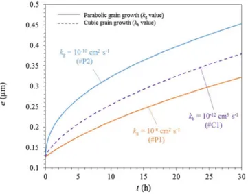
Fig. 5. effective chemical diffusion coefficient as a function of time for Ni-30Cr oxidized at 1173 K calculated by combining Eqs.(3),(4)and(9)or(12)assuming a parabolic oxide grain growth law for cases #P1 (kg= 10−6cm2s−1) and #P2 (kg= 10−10cm2s−1) and a
cubic oxide grain growth for case #C1 (kh= 10−12cm3s−1).
Fig. 6. effective chemical diffusion coefficient as a function of time for Ni-30Cr oxidized at 1173 K calculated by combining Eqs.(3),(4)and(9)or(12)assuming a cubic oxide grain growth for case #C2 (kh= 10−18cm3s−1) and a slow parabolic grain growth for
curves are more visible over short periods of time.
The higher the value of kgor kh, the slower the oxidation kinetics.
This tendency was expected. It seems interesting however to notice that the general shape of the oxidation curves evolves with the chosen value of kgor kh. For cases #P3 and #C3, which have the lowest values of kg
and khrespectively, oxidation kinetics move away from a parabolic law
and appears to be more of a sub-parabolic pattern as shown inFig. 10. For the highest values of kgand kh: 10−6cm2s−1and 10−12cm3s−1
respectively, oxidation kinetics look like a parabolic law as shown in Fig. 9. For the intermediate values of kg and kh: 10−10cm2s−1 and
10−18cm3s−1respectively, oxidation kinetics seem to display
inter-mediate shapes as shown inFigs. 9 and 10respectively.
4.3. Study of the combined effect of grain size gradient within the oxide scale and parabolic grain growth
In this part the three following cases were treated: (1) a parabolic grain growth law for case #P4 according to Eq. (9) with kg= 1.67 10−14cm2s−1, (2) a grain size gradient for case #G1 with
g1= 32 nm and g2= 95 nm; and (3) a combination of parabolic grain
size growth and grain size gradient for case #G1P4. These different oxidation kinetics are presented inFig. 11. They are plotted over short oxidation time periods of up to 20 h: this time window corresponds to the interest zone for the simulation parameters chosen.
During the very early stages of oxidation (up to 2 h), the oxide thickness corresponding to a parabolic growth law for case #P4 is higher than the oxide thickness corresponding to the grain size gradient for case #G1. After two hours, this tendency is reversed and the oxide thickness corresponding to the grain size gradient for case #G1 be-comes higher than the oxide thickness corresponding to the parabolic grain size growth for case #P4. This result shows that the two oxidation kinetics do not follow the same law. According to Eq.(26), the oxida-tion kinetics corresponding to a parabolic grain size growth is sub-parabolic, whereas according to Eq.(34), the oxidation kinetics corre-sponding to a grain size gradient remains purely parabolic.
Concerning case #G1P4, with the combination of parabolic grain size growth and grain size gradient, the oxide thickness is always smaller than that of the two other cases. This result was expected since in this case, the grain size cumulates both growth effects: in time and in space. The proportion of short-circuit diffusion is thus the lowest of the three cases. A similar conclusion can be made for a cubic grain growth law instead of a parabolic grain growth law.
Results from this section can be summarized as follows:
Fig. 7. effective chemical diffusion coefficient as a function of time for Ni-30Cr oxidized at 1173 K calculated by combining Eqs.(3),(4)and(12)assuming a slow cubic grain growth law for case #C3 (kh= 10−24cm3s−1).
Fig. 8. chromia growth kinetics on Ni-30Cr at 1173 K calculated with EKINOX and analytical models with g0= 32 nm, and kp,L= 1.18 10−14cm2s−1 for different
hy-potheses: a parabolic grain size growth for case #P4 according to Eq. (9) with kg= 1.67 10−14cm2s−1, a cubic grain growth law for case #C4 according to Eq.(12)
with kh= 1.69 10−18cm3s−1, and a grain size gradient for case #G1 with g1= 32 nm
and g2= 95 nm. An experimental data [10] is also displayed.
Fig. 9. oxidation kinetics of Ni-30Cr oxidized at 1173 K calculated with Eqs.(26)or(29)
assuming a parabolic oxide grain growth law for cases #P1 (kg= 10−6cm2s−1) and #P2
(kg= 10−10cm2s−1) and cubic oxide grain growth for case #C1 (kh= 10−12cm3s−1).
Fig. 10. oxidation kinetics of Ni-30Cr oxidized at 1173 K, calculated with Eqs.(26)and
(29)assuming a parabolic grain growth for case #P3 (kg= 10−14cm2s−1) and a cubic
- A parametric study with analytical calculations showed that kgand
khparameters, which characterize the grain growth rate, can have a
major influence on the shape of oxidation kinetic curves when considering the grain boundaries as a fast diffusion path.
- EKINOX calculations taking into account the combined effect of grain growth and grain size gradient across the oxide scale for case #G1P4, show that the resulting oxidation kinetics are closer to the oxidation kinetics corresponding to the grain size gradient only for case #P4 for short times, and closer to the oxidation kinetics cor-responding to grain growth only for case #G1 for longer times. Considering these points, it is interesting to discuss post-treatment methods of oxidation kinetics curves as well as derived extrapolations over a longer time range.
5. Discussion
The aim of this discussion is to compare two different methods of interpretation and extrapolation of experimental oxidation kinetics: the “log-log” method and the “parabolic law” method. To do so, the results of the previous calculations are used as if they were experimental data. 5.1. Estimation of the parabolic rate constant values (kp) from calculated
kinetic curves
In this paragraph, oxidation kinetics simulated with EKINOX pre-sented in the previous section are post-treated according to the “para-bolic law” method with the local kp calculation method [43]. This
method is presented in Section2.6.1. The oxidation kinetics considered for the calculation of local kpvalues for cases #P4, #G1 and #G1P4 are
plotted inFig. 11. Corresponding local values of kpare plotted over time
inFig. 12.
The local kpvalue corresponding to case #G1 with grain size
gra-dient across the oxide scale but without grain growth is constant. This result could have been predicted as the corresponding kinetics follows a pure parabolic law as determined in Eq.(34). The local kpvalue
cor-responding to the combination of a parabolic grain growth and a grain size gradient for case #G1P4, is close to the local kp curve
corre-sponding to a parabolic grain growth # P4. These two local kpcurves
corresponding to cases with a grain size evolution over time: cases #P4 and #G1P4, decrease rapidly of about one order of magnitude during thefirst hour of oxidation. It shows that for short time experiments the grain growth can strongly affect the value of the parabolic rate constant determined by a classicalfit on the whole kinetic curve. The fact that
the value of kpchanges over time could explain the discrepancy of kp
values found in the literature for different oxidation times as presented inFig. 1.
5.2. Treatment of oxidation kinetics obtained with EKINOX simulations, using several values for kgand kh
5.2.1. Log-log method
The usual way of using the“log-log” method is to perform a linear fit in a log–log plot on the whole kinetic curve. The “log-log” method is explained more extensively on Section 2.6.2. This method over-estimates the weight of short times on the global interpretation because of the logarithm function. For long term extrapolation, a more accurate description of oxidation kinetics can be obtained by admitting the ex-istence of a transitory regime for short times. Thus, linearfits are per-formed on the final portions of the plots, which better describe the stationary regime. In this part, the extrapolation using the“log-log” method is compared to the extrapolation using the “parabolic law” method that also uses thefinal part of the oxidation kinetic curve. For a fair comparison, this is carried out on the same time interval.
Examples of calculated oxidation kinetics are post-treated with the “log-log” method inFig. 13for the parabolic grain growth cases: #P1, #P2, and #P3. Linearfits are performed on a time range from 25 to 30 h. According to the“log-log” method, the parameters m and klog
from Eqs.(24)and(25)can be obtained. These values for the different oxidation kinetics corresponding to the different values of kgand khare
gathered inTable 3.
The parameter m reflects the shape of the oxidation kinetics as it corresponds to the value of the time exponent parameter according to Eq. (24). For the fastest grain growth conditions: #P1 with kg= 10−6cm2s−1and #C1 with kh= 10−12cm3s−1, the m parameter
equals 1.4 and 1.7 respectively, that means that the shape of the oxi-dation kinetics can be bounded between a linear dependence with time and a square root dependence with time. The global oxidation kinetics could thus be interpreted as an over-parabolic law. For the intermediate rate of grain growth with kg= 10−10cm2s−1 and the case with
kh= 10−18cm3s−1corresponding to cases # P2 and #C2 respectively,
the m value equals 2.15, and 2.8 respectively, that means that the shape of the oxidation kinetics can be bounded between a square root de-pendence with time and a cubic root dede-pendence with time. The oxi-dation kinetic law can be interpreted as parabolic (if m parameter is close to 2) or as an intermediate law between parabolic and cubic. For the slowest grain growth rate: case #P3 with kg= 10−14cm2s−1, the m
parameter equals 3.8, that means that the shape of the oxidation
Fig. 11. chromia growth kinetics of Ni-30Cr at 1173 K calculated with the EKINOX model corresponding to different hypotheses: a parabolic grain size growth for case #P4 (kg= 1.67 10−14cm2s−1), a grain size gradient for case #G1 with g1= 32 nm and
g2= 95 nm, and a combination of the parabolic grain size growth and grain size gradient
for case #G1P4.
Fig. 12. local kpfrom chromia growth kinetics of Ni-30Cr at 1173 K, calculated with the
EKINOX model corresponding to a parabolic grain growth for case #P4 (kg= 1.67 10−14cm2s−1), a grain size gradient for case #G1 with g1= 32 nm and
g2= 95 nm, and a parabolic grain size growth combined with a grain size gradient for
kinetics can be bounded between a cubic root dependence with time and a fourth root dependence with time. In this case, the oxidation kinetics is close to a quadratic law as the m parameter is close to 4. Finally for the slowest cubic growth rate: case #C3 with kh= 10−24cm3s−1, the m parameter equals 3.0, the oxidation kinetic
law can be interpreted as cubic, the shape of the oxidation kinetics can be approximated by a cubic root dependence with time. This last par-ticular case matches Rhines' observations [23,24] with a cubic grain growth law associated with a cubic oxidation kinetics. The grain size is thus proportional to the oxide thickness.
By using the“log-log” method, oxidation kinetics could be plotted with an over-parabolic, cubic or quadratic law despite the fact that growth mechanisms remain identical (only kinetic constants change).
These results can be explained by means of the analytical oxidation models presented in part II of this work: Eq.(26)for a parabolic oxide grain growth and Eq.(29)for a cubic oxide grain growth. The oxidation kinetic law given by Eq. (26) is composed of three terms. One term proportional to time, one term proportional to the square root of time, and one constant term. Depending on the values of the parameters of the law, one term of the kinetic law can become predominant compared to the others for a given time range, and the global oxidation kinetics follows the tendency given by the predominant term. If the pre-dominant term is the one proportional to time, the global oxidation
kinetics has a parabolic pattern, for example #P1 with kg= 10−6cm2s−1. If the predominant term is the one proportional to
the square root of time, the global oxidation kinetics has a quadratic pattern, for example #P3 with kg= 10−14cm2s−1. Transition values of
kgand khfrom one type of law to the other can be determined for a
given duration of the experiment. This calculation is described in Appendix B.
Some oxide thickness extrapolations from 30 h oxidation kinetics can be calculated according to kinetic laws using Eq.(24)with the data gathered inTable 3. The corresponding extrapolated oxide thickness for 1 year and 10 years of oxidation are gathered inTable 3. For compar-ison, real thicknesses from analytical laws(26) and(29) are also re-ported. Relative errors in the extrapolation range from 0.1% to 217%. The gap between extrapolated and analytical values increases with longer extrapolation times and with the values of kgand kh. Indeed, the
relative error is the highest for cases #P1 and #C1, which correspond respectively to the highest values of kgand kh.
5.2.2. Complete parabolic law method
Another post-treatment method applied to kinetic curves has been carried out by using Eq. (22), which corresponds to the complete parabolic law. This law has been adjusted tofit the curves on the same time interval as determined previously (for the“log-log” method): from 25 to 30 h. kp,(25h), values obtained following these adjustments are
listed inTable 3.
kp,(25h)values given inTable 3and obtained in the 25–30 h time
period are higher for cases with the lowest values of kgand kh. As grain
size increases continuously over time, the local kpvalue decreases over
time, and for a long enough time, the second part of Eqs.(26)and(29) become negligible compared to thefirst part of the relations. The kp,stat
value is expected to reach kp,L= 8.10−15cm2s−1for an infinite time. A
similar observation can be made on the values of the effective diffusion coefficient plotted inFigs. 5–7, which decrease over time with the grain growth. The effective diffusion coefficients are obviously expected to reach the lattice diffusion coefficient for an infinite time. In the cases studied here, the time needed to reach this stationary regime depends on grain growth kinetics, and is thus linked to the values of kgand kh. If
the grain growth is fast, the effective diffusion coefficient quickly reaches its stationary value. In contrast, if the grain growth is slow, the effective diffusion coefficient reaches its stationary value after a long time.
The kp,(25h)values obtained by parabolicfit gathered inTable 3for
cases #P1, #P2 and #C1 are of the same order of magnitude as kp,L= 8.10−15cm2s−1. It can thus be assumed that, in these cases, the
stationary regime is reached after 25 h. For cases #P3, #C2 and #C3 however, the local kpvalue is different from the kp,Lvalue, ranging from
one to three orders of magnitude. This is due to the fact that the sta-tionary regime has not been reached after 25 h. The kpvalues obtained
Fig. 13. oxidation kinetics of Ni-30Cr at 1173 K, calculated with Eq.(26), plotted on a log–log scale (e-e0(cm), t(s)) assuming a parabolic growth law according to Eq.(9), and
for kgvalues of 10−14cm2s−1, 10−10cm2s−1and 10−6cm2s−1. Linearfits are done for
the time interval going from 25 to 30 h. Solid lines correspond to calculated kinetics, dotted lines to linearfits.
Table 3
Analytical oxide thickness calculated with Eqs.(26)and(29)respectively for parabolic grain growth #P1, #P2, #P3 and cubic grain growth #C1, #C2, #C3. m, klog, and kp,(25h)
parameters are obtained from extrapolations of analytical oxidation kinetics of Ni-30Cr on 30 h at 1173 K according to“log-log” and “parabolic law” methods. Extrapolated oxide thicknesses corresponding to“log-log” and “parabolic law” extrapolation methods according to Eqs.(24)and(22)and calculated with parameters m, klogand kg,(25h)are given for 1 year
and 10 years. Finally, relative errors on oxide thickness between analytical and extrapolated values are given.
log–log method Parabolic law method Calculation case Oxide grain growth
parameter
Analytical oxide thickness (μm)
m klog elog-log(μm) Relative error on
oxide thickness (%)
kp,(25h)= 1/C
(cm2s−1)
eparablaw(μm) Relative error on
oxide thickness (%) 1 year 10 years 1 year 10 years 1 year 10 years 1 year 10 years 1 year 10 years #P1 kg (cm2s−1) 10−6 5.0 15.9 1.4 2.10−12 10.2 50.4 104 217 8.10−15 4.9 15.8 2 0.6 #P2 10−10 5.2 16.1 2.15 4.10−15 4.8 14.3 8 11 8.10−15 5.1 16.0 2 0.6 #P3 10−14 14.2 28.4 3.8 4.10−19 13.8 25.2 3 11 8.10−14 18.0 51.7 27 82 #C1 kh (cm3s−1) 10 −12 5.2 16.2 1.7 2.10−13 7.6 29.6 46 83 9.10−15 5.3 16.5 2 2 #C2 10−18 14.4 33.1 2.8 4.10−16 14.8 33.7 3 2 9.10−14 18.2 54.6 21 67 #C3 10−24 135.1 291.3 3.0 9.10−14 135.0 292.2 0.1 0.3 8.10−12 177.4 529.6 31 82
by parabolic fit for these three cases thus do not correspond to the stationary kp value. Consequently the parabolic extrapolation is not
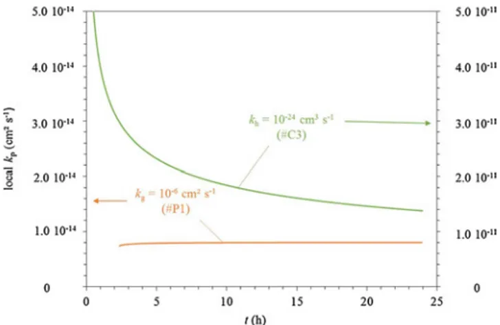
correct and should not be employed in these cases. The evolution of local kpvalues of cases #P1 and #C3 are plotted inFig. 14. In case #P1,
local kpis stationary throughout the entire time range chosen, whereas
in case #C3, the value of kpdecreases dramatically at early oxidation
times and is still decreasing at the end of the experiment. This illustrates that the stationary value of kphas not been reached at the end of the
oxidation time chosen here.
The oxide thickness can be extrapolated using complete parabolic laws with Eq.(22)and parameters given inTable 3. This same table displays the values of these extrapolated oxide thicknesses for 1 year and 10 years, and the corresponding analytical values calculated with Eqs.(26)and(29). The relative errors between extrapolated and ana-lytical values range from 0.6% and 82%. Contrary to the extrapolations obtained with the“log-log” method, discrepancies increase as values of kgor khdecrease. Indeed, the most important relative errors are found
for cases #P3, #C2 and #C3, those with the slowest grain growth rate, and therefore having the longest transient stage of oxidation. For the slowest grain growth rates, the oxidation kinetics is far from the para-bolic regime, even over a long time range. As shown inFig. 14with case #C3, local kphad still not reached its stationary value after 25 h.
To conclude this part, the best way tofit the experimental data is to use the local kp methodfirst, in order to determine if the parabolic
stationary regime is reached. If so, the best extrapolation is given by the complete parabolic law using the value of kpobtained for the stationary
regime, i.e. kp,stat. This method is more accurate than the one that uses a
power law, even if this latter has been obtained by a fit over longer oxidation times. If no parabolic stationary regime can be determined for the local kpcurve, as is the case for very slow grain growth rates, it can
be then more appropriate to use the“log-log” method for extrapolation.
However, when possible, the best method is to perform a longer ex-periment until the stationary regime is reached, and to extrapolate with the“parabolic law” method using the stationary kpand the complete
law. The alternative method consists in using an analytical or numerical model that includes grain growth kinetics, if the evolution of local kpis
assumed to be due to the oxide grain size evolution. 6. Conclusion
The conclusions that can be drawn from this work are the following: 1) Grain boundary diffusion and oxide scale microstructure evolution over time should be considered to interpret oxidation kinetics which are not purely parabolic.
2) Analytical models are presented considering a cubic grain growth law and a grain size gradient across the oxide scale. A numerical resolution, using for example the EKINOX model, can be used to simulate more complex cases of combination of grain size growth and grain size gradient but also other grain size growth laws. 3) Calculation results show that even when using the same oxide
growth mechanism, i.e. control by faster diffusion in the oxide due to grain boundaries diffusion, the evolution rate of diffusion short-circuit proportion over time modifies the oxide growth kinetics, and even their global shapes.
4) Depending on grain growth kinetics, the experimental oxidation kinetics that derive from a mixed diffusion phenomenon in bulk and in grain boundaries can be globally interpreted with various laws from over-parabolic to parabolic, sub-parabolic, cubic and even quadratic.
5) Extrapolation of oxidation kinetics can be strongly affected by the choice of the method, and also by the duration of the oxidation experiment. The use of the“local kp” helps identifying if the
para-bolic stationary regime is reached and thus helps performing accu-rate extrapolations of oxidation kinetics. If the stationary regime is not reached during the oxidation time of the experiment, no extra-polation should be done. If longer experiment cannot be performed, extrapolation using the“log-log” method might be a better choice. However, experimenters have to keep in mind that this extrapola-tion is not based on clearly identified rate controlling phenomena and then should be used with caution.
This study focuses on the growth of chromia, however, similar conclusions can be drawn on the growth of other oxides.
Acknowledgments
S. Gossé, C. Gueneau, P. Zeller and A. Chartier (CEA), for Thermocalc calculations and constructive discussions are gratefully acknowledged.
Appendix A. Symbols used
A, B, C: coefficients used for the “complete parabolic law fit” (respectively in s, s cm−1, s cm−2)
XAn: atomic site fraction of A in the slab n in the EKINOX model
XA: atomic site fraction of A (A = Cr or Ni) in alloy
CXn: site fraction for specie X calculated on EKINOX model in slab n (dimensionless)
∼
Deff: effective chemical diffusion coefficient (cm2s−1)
∼
Dgb: grain boundary chemical diffusion coefficient (cm2s−1)
∼
DL: chemical diffusion coefficient in oxide lattice (cm2s−1)
JXn:flux of specie X calculated on EKINOX model in slab n (site m−2s−1)
e: oxide scale thickness, e0corresponds to oxide thickness at initial time t0(cm)
f: atomic site fraction on short-circuits path per unit area (dimensionless)
g: grain size, g0grain size at initial time t0, g1corresponds to oxide grain size at metal/oxide interface, g2corresponds to oxide grain size at oxide/
gas interface (cm)
Fig. 14. local kpvalue corresponding to the oxidation kinetics of Ni-30Cr at 1173 K,
calculated with Eqs.(26)and(29), corresponding respectively to kg= 10−6cm2s−1for
kg: parabolic coefficient for the grain growth law (cm2s−1)
kh: cubic coefficient for the grain growth law (cm3s−1)
kl: linear constant of the oxide scale growth (cm s−1) or (g cm−2s−1)
klog: kinetic parameter used for the power law kinetics of oxide scale growth (“log-log” method) (units depend on exponent of the power law: m)
kp: parabolic constant of the oxide scale growth, kp,effcorresponds to effective parabolic constant in case of diffusion through lattice and grain
boundaries, kp,Icorresponds to instantaneous parabolic constant of the oxide scale growth, kp,Lcorresponds to parabolic constant of the oxide scale
growth in case of diffusion through lattice only, kp,statcorresponds to local parabolic constant corresponding to the stationary regime of the oxide
scale growth (cm2s−1) or (g2cm−4s−1)
m: exponent used for the power law kinetics of oxide scale growth (“log-log” method) (dimensionless) t: time, t0corresponds to initial time (s) or (h)
x: position in the oxide scale (cm)
δ: short-circuit thickness, or grain boundary thickness (cm)
ΔC: difference in defect concentration between the oxide/gas interface and the metal/oxide interface (atom cm−3)
Δm: mass gain per unit area, Δmicorresponds to initial mass gain per unit area (g cm−2)
ΔXV: difference between vacancy site fraction at oxide/gas and metal/oxide interfaces (dimensionless)
Δy: difference of relative position in oxide scale (dimensionless) Ω: volume of oxide per oxide site (cm3atom−1)
Appendix B. Calculation of transition kgand khvalues
With an oxidation time of 30 h, a transition kgvalue, so calledkgtrcan be determined for transition between predominance of the square root part
of time. Right side of Eq.(26)and predominance of the linear part of time i.e. left side of Eq.(26).
+ = − ∼ ∼ k t e δk ( 1) t k D D p,L 02 4 p,L gtr gb L (39) leading to: = ⎛ ⎝ ⎜ ⎜ + − ⎞ ⎠ ⎟ ⎟ ∼ ∼ k δk k t D D 4 ( 1) e t gtr p,L p,L gb L 2 02 (40) Following the same approach, the transition value of the cubic growth rate of grain sizekhtrleading to different regimes of oxidation kinetics can
be determined: = ⎛ ⎝ ⎜ ⎜ + − ⎞ ⎠ ⎟ ⎟ ∼ ∼ k δk k t D D 3 ( 1) e t tr p,L p,L 1/3 gb L 3 h 02 2/3 (41)
By using the parameters chosen in this study for case #P2, with kg= 10−10cm2s−1, global oxidation kinetics have a mixed parabolic and
quadratic tendency. For parameters corresponding to case #C2, with kh= 10−18cm3s−1, oxidation kinetics have a mixed parabolic and cubic
tendency.
In order to have the time proportionate term predominant in Eq. (26), the value of kgvalue must respect the condition: kg> >kgtr, this
corresponds to case #P1, with kg= 10−6cm2s−1. By using a similar approach for a cubic oxide grain growth law, the condition kh> >khtr
corresponds to case #C1, with kh= 10−12cm3s−1. These cases lead to oxidation kinetics following a parabolic law.
In order to have the term proportional to the square root of time predominant in Eq.(26), the value of kgmust respect the condition: kg< <kgtr,
this corresponds to case #P3, with kg= 10−14cm2s−1. By using a similar approach for a cubic oxide grain growth law, the condition kh> >khtr
corresponds to case #C3, with kh= 10−24cm3s−1. These cases lead to oxidation kinetics following a quadratic and a cubic law respectively.
Data availability
The processed data (output of EKINOX code) required to reproduce thesefindings, which are oxide thicknesses over time, and effective diffusion coefficient, are already shared in graphs inFigs. 8 and 11.
References
[1] A. Atkinson, R.I. Taylor, G. Simkovich, V.S. Stubican (Eds.), Transport in Nonstoichiometric Compounds, vol. 129, 1985, pp. 285–295. [2] K.P. Lillerud, P. Kofstad, J. Electrochem. Soc. 127 (1980) 2410–2419. [3] D.J. Young, M. Cohen, J. Electrochem. Soc. 124 (1977) 769–774.
[4] L. Cadiou, J. Paidassi, Mem. Scient. De La Revue De Metall. 66 (3) (1969) 217–225. [5] D. Caplan, G.I. Sproule, Oxid. Met. 9 (5) (1975) 459–472.
[6] C.A. Phalnikar, E.B. Evans, W.M. Baldwin, J. Electrochem. Soc. 103 (1956) 429–438.
[7] E.A. Gulbransen, K.F. Andrew, J. Electrochem. Soc. 99 (10) (1952) 402–406. [8] K. Taneichi, T. Narushima, Y. Iguchi, C. Ouchi, Materi. Trans. 47 (10) (2006)
2540–2546.
[9] A.C.S. Sabioni, J.N.V. Souza, V. Ji, F. Jomard, V.B. Trindade, J.F. Carneiro, Solid State Ionics 276 (2015) 1–8.
[10] S.C. Tsai, A.M. Huntz, C. Dolin, Mater. Sci. Eng. A 212 (1996) 6–13. [11] A.M. Huntz, A. Reckmann, C. Haut, C. Sévérac, M. Herbst, F.C.T. Resende,
A.C.S. Sabioni, Mater. Sci. Eng. A 447 (1–2) (2007) 266–276.
[12] M. Kemdehoundja, J.F. Dinhut, J.L. Grosseau-Poussard, M. Jeannin, Mater. Sci. Eng. A435 (2006) 666–671.
[13] E. Schmucker, C. Petitjean, L. Martinelli, P.J. Panteix, S. Ben Lagha, M. Vilasi, Corros. Sci. 111 (2016) 474–485.
[14] W.C. Hagel, A.U. Seybolt, J. Electrochem. Soc. 108 (12) (1961) 1146–1152. [15] G.M. Ecer, G.M. Meier, Oxid. Met. 13 (2) (1979) 119–158.
[16] L. Latu-Romain, Y. Parsa, S. Mathieu, M. Vilasi, A. Galerie, Y. Wouters, Corros. Sci. 126 (2017) 238–246.
[17] R.E. Lobnig, H.P. Schmidt, K. Hennesen, H.J. Grabke, Oxid. Met. 37 (1/2) (1992) 81–93.
[18] J.M. Perrow, W.W. Smeltzer, J.D. Embury, Acta Metall. 16 (1968) 1209–1218. [19] E. Essuman, G.H. Meier, J. Zurek, M. Hansel, T. Norby, L. Singheiser,
[20] K. Przybylski, G.J. Yurek, J. Electrochem. Soc. 135 (2) (1988) 517–523. [21] E.W. Hart, Acta Metall. 5 (1957) 595.
[22] R.J. Hussey, G.I. Sproule, D. Caplan, M.J. Graham, Oxid. Met. 11 (2) (1977) 65–79. [23] F.N. Rhines, R.G. Connell Jr., J. Electrochem. Soc. 124 (1977) 93–105. [24] F.N. Rhines, R.G. Connell Jr., M.S. Choi, J. Electrochem. Soc. 126 (6) (1979)
1061–1066.
[25] D.E. Davies, U.R. Evans, J.N. Agar, Proc. Roy. Soc. A225 (1954) 443–462. [26] W.W. Smeltzer, R.R. Haering, J.S. Kirkaldy, Acta Metall. 9 (1961) 880–885. [27] S. Hallström, M. Halvarsson, L. Höglund, T. Jonsson, J. Agren, Solid State Ionics 240
(2013) 41–50.
[28] P. Kofstad, K.P. Lillerud, J. Electrochem. Soc. 127 (11) (1980) 2410–2419. [29] M.W. Barsoum, J. Electrochem. Soc. 148 (2001) C544–C550.
[30] J.L. Smialek, Corros. Sci. 91 (2015) 281–286.
[31] R. Peraldi, D. Monceau, B. Pieraggi, Oxid. Met. 58 (2002) 249–273.
[32] D. Naumenko, B. Gleeson, E. Wessel, L. Singheiser, W.J. Quadakkers, Metall. Mater. Trans. A 38A (2007) 2974–2983.
[33] H. Larsson, T. Jonsson, R. Naraghi, Y. Gong, R.C. Reed, J. Agren, Mater. Corros. 68 (2) (2017) 133–142.
[34] T.J. Nijdam, W.G. Sloof, Acta Mater. 55 (2007) 5980–5987.
[35] T.J. Nijdam, L.P.H. Jeurgens, W.G. Sloof, Acta Mater. 51 (2007) 5295–5307. [36] C. Desgranges, N. Bertrand, K. Abbas, D. Monceau, D. Poquillon, et al., P. Steinmetz
(Ed.), High Temperature Corrosion and Protection of Materials 6, Prt 1 and 2, Proceedings, Trans Tech Publications Ltd, 2004, pp. 481–488 461–464. [37] N. Bertrand, C. Desgranges, M. Nastar, G. Girardin, D. Poquillon, D. Monceau,
P. Steinmetz, I.G. Wright, A. Galerie, D. Monceau, S. Mathieu (Eds.), High Temperature Corrosion and Protection of Materials 7, Pts 1 and 2, Trans Tech Publications Ltd, 2008, pp. 463–472 595–598.
[38] C. Desgranges, F. Lequien, E. Aublant, M. Nastar, D. Monceau, Oxid. Met. 79 (2013) 93–105.
[39] Y. Adda, J. Philibert, La Diffusion dans les solides Bibliothèque Des Sciences Et Techniques Nucléaires, Institut National Des Sciences Et Techniques Nucléaires & Presses Universitaires De France, Paris, 1966.
[40] C. Wagner, Zeitshrift für Physik B21 (25) (1933).
[41] I. Kaur, Y. Mishin, W. Gust, Fundamentals of Grain and Interphase Boundary Diffusion, John Wiley, 1995.
[42] L.G. Harrison, Trans. Faraday Soc. 57 (1961) 1191–1199. [43] D. Monceau, B. Pieraggi, Oxid. Met. 50 (1998) 477–493. [44] B. Pieraggi, Oxid. Met. 27 (1987) 177–185.
[45] A. Atkinson, R.I. Taylor, A.E. Hugues, Philos. Mag. A 45 (5) (1982) 823–833. [46] J. Zurek, D.J. Young, E. Essuman, M. Hänsel, H.J. Penkalla, L. Niewolak,
W.J. Quadakkers, Mater. Sci. Eng. A 477 (2008) 259–270.
[47] D.J. Young, D. Naumenko, L. Niewolak, E. Wessel, L. Singheiser, W.J. Quadakkers, Mater. Corros. 61 (10) (2010) 838–844.
[48] L. Kjellqvist, M. Selleby, CALPHAD 33 (2009) 393–397.
[49] A.C.S. Sabioni, R.P.B. Ramos, V. Ji, F. Jomard, W.A.A. Macedo, P.L. Gastelois, V.B. Trindade, Oxid. Met. 78 (2012) 211–220.