Using X-ray Computed Tomography to Describe the Dynamics of Nitrous Oxide Emissions during Soil Drying

HAL Id: insu-01241590

https://hal-insu.archives-ouvertes.fr/insu-01241590

HAL is a multi-disciplinary open access archive for the deposit and dissemination of sci-entific research documents, whether they are pub-lished or not. The documents may come from teaching and research institutions in France or abroad, or from public or private research centers.

L’archive ouverte pluridisciplinaire HAL, est destinée au dépôt et à la diffusion de documents scientifiques de niveau recherche, publiés ou non, émanant des établissements d’enseignement et de recherche français ou étrangers, des laboratoires publics ou privés.

Eva Rabot, Marine Lacoste, Catherine Hénault, Isabelle Cousin

To cite this version:

Eva Rabot, Marine Lacoste, Catherine Hénault, Isabelle Cousin. Using X-ray Computed Tomog-raphy to Describe the Dynamics of Nitrous Oxide Emissions during Soil Drying. Vadose Zone Journal, Soil science society of America - Geological society of America., 2015, 14 (8), 10 p. �10.2136/vzj2014.12.0177�. �insu-01241590�

For Review Only

Using X-ray computed tomography to describe the dynamics of nitrous oxide emissions during soil drying

Journal: Vadose Zone Journal Manuscript ID: VZJ-2014-12-0177-ORA.R1 Manuscript Type: Original Research Articles Date Submitted by the Author: 10-Apr-2015

Complete List of Authors: RABOT, Eva LACOSTE, Marine Henault, Catherine Cousin, Isabelle

Keywords: soil, nitrous oxide, X-ray computed tomography, gas diffusivity, pore connectivity

For Review Only

Using X-ray computed tomography to describe the dynamics of nitrous oxide emissions 1

during soil drying 2

E. Rabot1,2, M. Lacoste2, C. Hénault2, I. Cousin2,* 3

1

Laboratoire Léon Brillouin, UMR12, CEA Saclay, 91191 Gif-sur-Yvette Cedex, France 4

2

INRA, UR0272, UR Science du Sol, F-45075 Orléans, France 5

* Corresponding author: isabelle.cousin@orleans.inra.fr 6

Impact statement 7

We proposed a methodology to image the water dynamics and the soil structure of a soil 8

sample with X-ray computed tomography, while controlling the hydric state and monitoring 9

N2O fluxes. Relevant information about N2O transport could be extracted from the images.

10

Abstract 11

Water in soil is known to be a key factor for controlling nitrous oxide (N2O) emissions, 12

because N2O is mainly produced by denitrification in anoxic environments. In this study, we 13

proposed a methodology to image the water and soil structure of a soil sample with X-ray 14

computed tomography, while controlling the hydric state and monitoring N2O fluxes. We

15

used a multistep outflow system to apply two wetting-drying cycles to an undisturbed soil. 16

The soil core was scanned with coarse-resolution X-ray computed tomography, one time 17

during wetting and several times during drying, to measure quantitative and qualitative 18

indicators of the pore network. Nitrous oxide emissions were higher during the first (C1) than 19

during the second (C2) wetting-drying cycle, both for the wetting and the drying phases. 20

Fluxes increased quickly after the beginning of the drying phase to reach a peak after 5 h. 21

Differences in the intensity of N2O emissions between the two cycles were attributed to

22

differences in the water saturation, air-phase connectivity, and relative gas diffusion 23

coefficient, which led to more or less N2O production, consumption, and entrapment in soil.

24

The speed of the N2O emissions at the beginning of the drying phase depended on the rate of

25

increase of the air-filled pore volume and connectivity, and was especially well described by 26

the estimated relative gas diffusion coefficient. Parameters of the soil structure were not able 27

to explain completely the intensity of N2O emissions during drying: N2O production and

28

consumption factors were also involved. 29

For Review Only

Abbreviations: C1: first wetting-drying cycle; C2: second wetting-drying cycle; WFPS: 30

water filled pore space. 31

1 Introduction 32

Nitrous oxide (N2O) concentration in the atmosphere is constantly increasing (Khalil et al., 33

2002). With a global warming potential 300 times higher than that of carbon dioxide over a 34

100-year time scale (World Meteorological Organization, 2007), N2O is the gas with the third 35

largest contribution to global warming (Ciais et al., 2013). Nitrous oxide plays also an 36

important role in the stratospheric ozone depletion (Ravishankara et al., 2009). Soils are a 37

major source of N2O, accounting for 60% of natural sources (soils under natural vegetation) 38

and 60% of anthropogenic sources (soils used for agriculture; Ciais et al., 2013). Nitrous 39

oxide is produced during the natural microbial reactions of nitrification and denitrification, 40

two reactions which are controlled by the status of aerobiosis in soils. Since the water 41

saturation of soils modifies the ratio between filled and air-filled pore space, the water-42

filled pore space (WFPS) is often used as an indicator of N2O emissions (Butterbach-Bahl et

43

al., 2013; Robertson, 1989). In particular, wetting and drying cycles are known to affect N2O

44

emissions (Guo et al., 2014; Muhr et al., 2008). Peaks of N2O emissions have often been 45

observed both in the field and in laboratory experiments after the rewetting of a soil 46

(Groffman and Tiedje, 1988; Sanchez-Martin et al., 2010; Sexstone et al., 1985). 47

Following the model proposed by Smith (1980), N2O production can occur inside anoxic

48

aggregates and then diffuse to the soil surface through inter-aggregate pores. Thus, delays 49

between microbial production and the moment when N2O can be measured at the soil surface

50

have been demonstrated (Clough et al., 1998; McCarty et al., 1999; Rabot et al., 2014; Weier 51

et al., 1993; Wollersheim et al., 1987). Delays in N2O emissions are partly linked to gas

52

entrapment and the associated dissolution of N2O in the water phase (Clough et al., 2005). We

53

hypothesize here that introducing dynamic indicators of the soil structure could enhance our 54

For Review Only

understanding of the dynamic nature of N2O emissions during wetting and drying cycles, by a

55

better description of N2O transport. Indeed, since soil structure controls the water and gas

56

dynamics in soils, and thus the aerobic microbial activity, soil structure is supposed to be of 57

great importance for N2O emissions (Ball, 2013). 58

Both the soil water and soil structure can be studied by X-ray computed tomography. X-ray 59

computed tomography is rapid, non-destructive, and allows successive scans over time while 60

measuring other dynamic parameters, such as N2O fluxes. It provides 3-D images, used to 61

perform spatial analysis of the soil sample. In soil science, X-ray computed tomography is a 62

common tool, used for example to study the effect of agricultural practices (Deurer et al., 63

2009; Schjønning et al., 2013; Schlüter et al., 2011), the water dynamics (Kasteel et al., 2000; 64

Sammartino et al., 2012; Wildenschild et al., 2005), or the gas dynamics (Deurer et al., 2009; 65

Katuwal et al., 2014; Naveed et al., 2013). Katuwal et al. (2014) demonstrated the interest of 66

coarse-resolution X-ray scanners to study gas transport functioning in macropores. This 67

methodology can be applied to N2O emissions. Only few studies used imaging techniques to

68

study greenhouse gas emissions (e.g., Mangalassery et al., 2014; Mangalassery et al., 2013), 69

and to our knowledge, none of them monitored greenhouse gases while acquiring images of 70

the soil structure. 71

In this study, we proposed a methodology to image the water and soil structure of a soil 72

sample with coarse-resolution X-ray computed tomography, while controlling the hydric state 73

and monitoring N2O fluxes. We aimed at demonstrating which relevant information can be 74

extracted from the images to allow a better understanding of N2O emissions. We illustrated

75

this methodology by subjecting a soil sample to two wetting and drying cycles. 76

For Review Only

77

2.1 Soil sampling, physical and chemical characterization

78

The study site was chosen for the high N2O emissions previously recorded in the field (Gu et 79

al., 2011), at the same location as the study of Rabot et al. (2014). The site is an agricultural 80

field cultivated with rape (Brassica napus L.), located near Chartres, in the northwest of 81

France (48.376° N lat, 1.196° E long). The soil is classified as Glossic Retisol (WRB, 2014), 82

with a clay content of 13.7%, a silt content of 82.0%, and a sand content of 4.3% (Rabot et al., 83

2014). A soil core was collected in June 2013 in a PVC cylinder (13.2-cm inner diameter by

84

7-cm height) from the surface horizon (1–8 cm). Bulk soil was also sampled in the surface 85

horizon for physical and chemical analyses. Soil organic carbon was measured by 86

sulfochromic oxidation, and total nitrogen was measured by the Dumas method. The soil 87

nitrate content was determined by colorimetric analysis after the extraction from an 8-g soil 88

sample using 0.5 M K2SO4. Soil pH was determined in a 1:2.5 soil/water volume ratio on

89

samples sieved at < 2 mm. At the sampling time, the soil organic carbon was 9.5 g kg–1, the

90

total nitrogen content was 0.91 g kg–1, the nitrate content was 51.3 mg NO3−–N kg–1, and the 91

soil pH was 5.6. The porosity of the soil sample was 0.46 cm3 cm−3 and the volumetric water

92

content was 37.7% (equivalent to 81.9% WFPS). The sample was conditioned in a plastic bag 93

and stored field moist during two weeks at 5°C to minimize microbial activity. Before the 94

start of the experiment, the soil core was trimmed on each end and maintained at 20°C for 24 95

h. 96

2.2 Experimental setup 97

The experiment consisted in controlling the hydric status of the soil sample with a multistep 98

outflow system (Weihermüller et al., 2009): the soil cylinder was connected to a water-tank to 99

control its wetting according to the Mariotte bottle principle, and connected to a vacuum 100

For Review Only

pump and a sampling bottle to control its drying (Fig. 1). Hydraulic continuity was ensured 101

with a porous ceramic plate (1-bar air-entry value, 8.6 × 10–8 m s–1 saturated hydraulic 102

conductivity, Soilmoisture Equipment Corp.) placed at the bottom of the soil cylinder and 103

previously saturated with water. The soil cylinder-ceramic plate system was sealed with 104

silicon to avoid water or gas leaks. Both the water content and water potential were 105

continuously monitored during the experiment, with a balance (0.1 g precision) and two 106

microtensiometers (porous ceramic cup, 20-mm length, 2.2-mm diam., 150-kPa air-entry 107

value) inserted at 2 and 4 cm from the cylinder surface at the end of the wetting phase. Data 108

were recorded every 10 min with a datalogger (CR1000, Campbell Scientific). 109

Two wetting-drying cycles (hereafter referred to as the C1 and C2 cycles) were applied to the 110

soil cylinder. The initial water content for C1 was the water content at sampling. The sample 111

was first saturated for 3 d by raising the water level to the soil surface in one step, and then a 112

–100 hPa pressure was applied at the bottom of the soil core in one step, and maintained for 113

about 7 h (C1 cycle). A zero hPa pressure was then applied for 3 d, followed by a –100 hPa 114

pressure for about 7 h (C2 cycle). Indeed, Rabot et al. (2014) demonstrated that N2O peaks

115

can be created during the drying phase, at a matric potential of approximately −50 hPa. We 116

chose thus to apply a pressure lower than this value of −50 hPa. The speed of the matric 117

potential decrease was much higher that under natural conditions, and could affect the water 118

transport and hydraulic continuity. We used a KNO3 solution as the wetting fluid, to ensure

119

that nitrate was not a limiting factor for N2O emissions during the wetting phase, and to

120

isolate the effects of nitrate concentration and soil moisture on the N2O emissions. Hénault

121

and Germon (2000) showed that the response of N2O emissions to the nitrate concentration

122

could be described by a Michaelis-Menten function. We used a nitrate concentration at the 123

plateau of this function (4.1 mM N). The nitrate solution was prepared with de-aired water to

124

prevent air bubble formation during the experiment. 125

For Review Only

Nitrous oxide emissions were monitored by infrared correlation spectroscopy (N2O Analyzer 126

model 46i, Thermo Scientific) using a 4-L volume closed-chamber. The emissions were 127

measured for 20-min periods, and the concentration value was recorded every minute. Given 128

the linear increase of the N2O concentration in the closed-chamber, N2O fluxes were 129

calculated linearly from the observed change in concentration during the first 10 min after the 130

chamber was closed. Only one N2O flux measurement was done during wetting, at the end of 131

each wetting phase for each cycle, and seven (respectively eight) flux measurements were 132

recorded during the drying phase for the C1 (respectively C2) cycle. Moreover, gases inside 133

the chamber were sampled in evacuated vials at the end of the wetting phase and at the middle 134

of the drying phase (3.5 h after the beginning of the drying phase), and CO2 concentration was 135

determined by gas chromatography (µGC Gas Analyzer T-3000, SRA Instruments). For a 136

single CO2 flux measurement, the atmosphere of the closed-chamber was sampled three times

137

during 20-min periods. Given the linear increase of the CO2 concentration, the flux was then

138

calculated linearly. The chamber was removed before each measurement to restore the

139

atmosphere to ambient concentrations of gases. The sample was kept inside the scanner 140

during the two wetting-drying cycles. The temperature inside the scanner room was monitored 141

and ranged between 22.5 and 25.5°C throughout the experiment.

142

2.3 Computed tomography and image analyses 143

The soil sample was placed in the scanner in its sampling direction. The soil sample was 144

scanned one time at the end of the wetting phase, and the vacuum pump was then activated to 145

begin the soil drying. We then scanned the sample seven times for C1, and nine times for C2 146

during the drying phase, alternating with N2O flux measurements. Two scans have been added 147

at C2 compared to C1 to refine the results just after the beginning of the drying phase. We 148

used a medical X-ray tomograph (Siemens Somatom Definition AS) operating at an energy 149

For Review Only

level of 200 kV and a current of 140 mA. The voxel size was 316×316×100 µm. The scanning 150

duration was 15 seconds. In the following, intensities are expressed in Hounsfield units (HU). 151

Most of the image processing was realized with the ImageJ software (Rasband, 1997-2014). 152

Due to the chamber manipulation during the experiment and displacement of the sample 153

between scans, image registration was first done to ensure spatial consistency between the 154

different images with the Align3 TP plugin (Parker, 2012). We cropped the images to exclude 155

non-soil areas, and we rescaled the images to get isotropic voxels of 316 µm. The noise was

156

reduced by using a bilateral filter, and edges were enhanced with an unsharp mask (Schlüter 157

et al., 2014). The air phase and the water phase were both separated from the soil matrix and 158

gravels by using the watershed segmentation method. This method has previously been 159

successfully used to segment images of soils (Schlüter et al., 2014). A majority filter with a 160

3×3×3 kernel was applied to remove very small air-filled and water-filled pores which can be 161

seen as noise. We finally removed manually the signal of the two tensiometers. The procedure 162

used to segment the air phase and the water phase gave satisfactory results (Fig. 2). 163

Visualization of the air-filled and water-filled pore network was done with the ImageJ plugin 164

3-D Viewer (Schmid et al., 2010). 165

The volume of air-filled and water-filled macropores was estimated with the BoneJ plugin 166

(Doube et al., 2010), and the Euler number was calculated considering 26-connectivity with 167

the C library QuantIm v.4 (Vogel, 2008), on the segmented images. The Euler number 168

characterizes the connectivity of the air-filled pore space (Vogel et al., 2010). When the Euler 169

number is positive, the pore network is classified as unconnected, whereas it is connected 170

when the Euler number is negative. The volume of air-filled macropores and Euler number 171

were calculated on the total air-filled pores identified, and the air-filled pores connected to the 172

soil surface only, to evaluate the pore network contributing to N2O emissions. We estimated 173

the relative gas diffusion coefficients DS/D0 from the segmented air-filled pore space with

For Review Only

QuantIm v.4 (Vogel, 2008), as already done by Deurer et al. (2009) and Vogel et al. (2002). 175

The gas diffusion was modeled by using the Fick’s law of diffusion in 3-D, solved by explicit 176

finite differences. Throughout the simulation, the gas concentration at the bottom of the soil 177

sample was fixed at a constant value, and the gas concentration at the top was set to zero. We 178

calculated DS/D0 on subsamples of increasing thickness from the soil surface (adding 10

179

pixels at the bottom of the given subsample). 180

3 Results 181

3.1 Soil water content and soil water potential evolution 182

During the drying phase, the WFPS measured with the MSO system ranged between 85% and 183

79% at C1, and between 83% and 79% at C2. The soil matric potential was above 0 cm for 184

the two wetting cycles for the –4 cm depth tensiometer, whereas it was slightly under 0 cm for 185

the –2 cm depth tensiometer at C2 (Fig. 3). Saturation was thus slightly lower during C2. The 186

matric potential showed a plateau at the C2 wetting phase, reached in approximately 4.5 h 187

after the beginning of the C2 wetting phase. During the drying phase, the matric potential 188

decreased linearly, immediately after activating the vacuum pump, to reach –56 cm water 189

column at C1 and –67 cm water column at C2. The decrease of the matric potential was 190

slightly faster at C2 than at C1 (mean decrease of –8.8 cm h–1 at C1, and –9.5 cm h–1 at C2). 191

3.2 Dynamics of the N2O and CO2 fluxes

192

Emissions were lower during C2 than during C1, both for the wetting and the drying phases, 193

with the maximum N2O flux being 55.1 mg N m–2 d–1 at C1, and 19.1 mg N m–2 d–1 at C2 194

(Fig. 3). Nitrous oxide fluxes were measured to be 9.4 and 0.1 mg N m–2 d–1 at the end of the 195

C1 and C2 wetting phase, respectively. In comparison, they ranged between 0 and 2.6 mg N 196

m‒2 d‒1 in the field measurements of Gu et al. (2011) on the same study site. Nitrous oxide 197

For Review Only

fluxes increased quickly during the drying phase to reach a peak approximately 5.5 h after the

198

beginning of the soil drying at C1, and 4.5 h at C2. Peaks occurred at a mean matric potential 199

of –41.1 cm water column at C1, and –44.7 cm at C2, and at a WFPS of 80.2% at C1 and 200

80.5% at C2. The increase in the N2O fluxes was faster for C1 than for C2. The first flux

201

measurement of C1 was especially high (38.2 mg N m–2 d–1) compared to the following 202

measurements. At C2, the fluxes measured at the beginning of the drying phase increased 203

more slowly, with fluxes between 3.3 and 3.9 mg N m–2 d–1 for the three first measurements. 204

Carbon dioxide fluxes were higher at C2 than at C1 at the end of the wetting phase (50.4 mg 205

CO2 m–2 d–1 at C1, and 164.1 mg CO2 m–2 d–1 at C2). An opposite trend was observed during 206

the drying phase: CO2 fluxes were higher at C1 than at C2 (108.3 mg CO2 m–2 d–1 at C1, and 207

76.1 mg CO2 m–2 d–1 at C2). Soil pH at the end of the two wetting-drying cycles was 5.9. 208

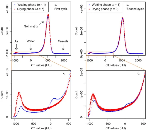
3.3 Characterization of the pore network 209

Four components could be identified, both visually and in the histograms of each image: air 210

phase, water phase, soil matrix, and gravels (Fig. 4 and 5). We define the soil matrix as the 211

solid phase and pores with a size lower than the image resolution. Histograms appeared to be 212

unimodal, with the mode corresponding to the soil matrix, because the air-filled and water-213

filled porosities represented only a small fraction of the soil sample volume (Fig. 4a and 4b). 214

A small peak near the pure air intensity value (–1024 HU) could be identified for the drying 215

phase, and a small peak near the pure water intensity value (0 HU) could be identified for the 216

wetting phase (Fig. 4c and 4d). Less water voxels and more air voxels were identified at C2 217

than at C1 during the wetting phase, showing that the water saturation was lower at C2 (Fig. 218

4c and 4d). 219

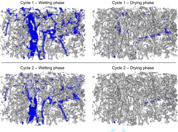
A 3-D rendering of the air phase and water phase distributions at the end of the wetting phase 220

and at the end of the drying phase for C1 and C2 is given in Fig. 5. Cylindrical pores, 221

For Review Only

probably earthworm burrows and root channels (of which one major root channel of 222

approximately 9 mm diameter), as well as smaller pores attributed to inter-aggregate voids are 223

visible. As expected, air-filled pores appeared to be more numerous at the end of the drying 224

phase than at the end of the wetting phase. A high volume of pore remained not saturated 225

during the experiment. 226

Most of the indicators calculated from the segmented images were highly correlated, except 227

the Euler number and DS/D0 (Table 1). Indeed, largest pores highly contributed to the

228

porosity, but relatively little to Euler number (Vogel et al., 2002), and DS/D0 includes

229

additional information about the tortuosity. The air-filled porosity identified ranged between

230

0.029 and 0.035 cm3 cm−3 at C1, and between 0.023 and 0.035 cm3 cm−3 at C2. In the driest

231

scan of C2, where the maximum air-filled pore volume has been identified, this air-filled 232

porosity is equivalent to 16% of the real air-filled porosity at a pressure of ‒100 hPa, or 7.5%

233

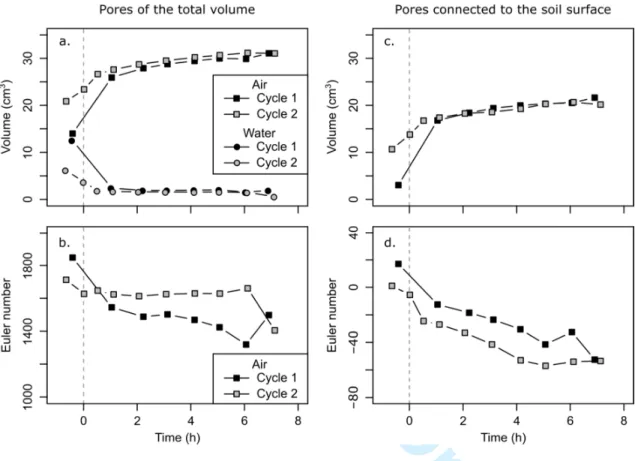
of the total porosity (0.46 cm3 cm−3). For the total core volume, time-evolution of the air-234

filled pore volume showed a rapid rise from the beginning to 1 h after the soil drying, and 235

then the system entered a state of equilibrium (Fig. 6a). C1 and C2 followed the same trend, 236

but the air-filled pore volume was significantly higher at C2 than at C1 at the end of the 237

wetting phase, and slightly higher at C2 than at C1 during the drying phase. The volume of 238

water-filled pores decreased quickly in the first hour of soil drying, and remained lower at C2 239

than at C1 during the whole experiment (Fig. 6a). The evolution of the air-filled pores 240

connected to the soil surface showed the same trend as for the total core volume, except that

241

no more difference can be seen between C1 and C2 after 2 h of soil drying (Fig. 6c). 242

For the total air-filled pore volume identified, the Euler number ranged between 1319 and 243

1849 at C1, and between 1405 and 1713 at C2 (Fig. 6b). Thus, the Euler number was positive 244

during the whole experiment, meaning that the air-filled pore network was unconnected at the 245

resolution of the images. The Euler number was lower at C2 than at C1 during the wetting 246

For Review Only

phase, and higher at C2 than at C1 during the drying phase. The air-filled pore connectivity 247

was thus better at C1 during the drying phase. The value of the Euler number tended to 248

decrease with soil drying. For the air-filled pores connected to the soil surface only, the Euler

249

number ranged between −52.5 and 17 at C1, and between −57 and 1 at C2 (Fig. 6d). A 250

transition between an unconnected and a connected pore network occurred in the first hour of 251

soil drying: the Euler number was positive at the end of the wetting phase, and negative 252

during the drying phase. The inherent connectivity improved then as the soil dried. The Euler 253

number was higher at C1 than at C2 during the whole experiment. One major pore cluster, 254

representing 98% of the air-filled pore volume connected to the soil surface at the end of the 255

two drying phases, was responsible for the negative value of the Euler number. The other 256

pores were smaller and had a less complicated morphology. 257

Simulated relative gas diffusion coefficients were null for subsamples thicker than 258

approximately 3 cm at C1, and 4 cm at C2, because deepest pores were poorly connected to 259

the soil surface. Thus, only the upper part of the soil sample could participate to the fast N2O

260

transport to the soil surface in the gaseous phase. The evolution with time of the gas diffusion 261

coefficient of a 3-cm-thick subsample is given in Fig. 7. Absolute values of DS/D0 ranged

262

between 0.000 and 0.009 at C1, and between 0.003 and 0.005 at C2. They were higher at C2 263

than at C1, except for the first measurement of the C1 drying phase. Relative gas diffusion 264

coefficients increased quickly after the beginning of the soil drying at C1, and then showed 265

lower values. This peak at C1 was concomitant with a fast increase of the N2O flux. The

266

increase with soil drying was slower at C2 than at C1. Trends were similar for the estimation 267

of DS/D0 on thinner subsamples (data not shown).

For Review Only

269

4.1 The use of X-ray computed tomography for greenhouse gas emission studies 270

The experiment of the present study appeared as the first report of coupling between soil 271

imaging, greenhouse gas flux measurements, and hydric control measured on the same 272

sample. The use of X-ray computed tomography allowed identifying spatially the water and

273

gas phases in the macropores, and thus determining the air-filled pore volume of these

274

macropores at successive moments during the soil drying. At the scanner resolution, only 16%

275

of the real air-filled porosity was identified, and the rest remained unresolved. Indeed, we 276

used a large sample, with a size typical of that used to determine soil hydraulic properties, to 277

approach the representative elementary volume of the soil. The pixel size was thus coarse, 278

approximately 300 µm. With such a resolution, only macropores are unequivocally 279

recognized, i.e., pores > 300 µm with the nomenclature of Jarvis (2007). According to Young-280

Laplace law (assuming 0° degree contact angle, interfacial tension for air-water and spherical 281

interfaces), these macropores are expected to drain at a water potential of ‒10 cm. 282

Identifying a higher range of pore sizes would have been informative since macropores

283

participate to N2O transport, whereas N2O production rather occurs in fine pores of the matrix 284

domain (Heincke and Kaupenjohann, 1999). However, such a coarse resolution has

285

successfully been used in previous studies to link soil structure and gas diffusion. By using X-286

ray computed tomography at a resolution of approximately 500 µm, Katuwal et al. (2014) 287

observed a high positive correlation between air permeability and the air-filled macroporosity 288

identified in their images. Deurer et al. (2009) explained a major part of the variability of the 289

gas diffusion coefficients by the air-filled porosity and connectivity of pores > 300 µm 290

identified with imaging. In the present study, despite the significant fraction of the unresolved 291

pores which were air-filled at the end of the two drying cycles, coarse-resolution X-ray 292

computed tomography can be used to infer N2O transport functioning. We also succeeded in

For Review Only

identifying differences in the soil moisture between the two wetting-drying cycles. This 294

difference was consistent with the other parameters recorded, i.e., matric potential and WFPS, 295

and allowed inferring differences in anoxia level in the soil profile between C1 and C2. 296

Relative, instead of absolute, comparisons between the two wetting-drying cycles could thus 297

be performed. 298

4.2 Nitrous oxide emissions and pore connectivity 299

After 3 days of water saturation, soil drying down to –45 cm water column induced maximum 300

N2O fluxes. This result has been previously observed by Rabot et al. (2014). They 301

hypothesized that the gas diffusion coefficient increased as the soil dried and allowed the 302

release of the N2O previously entrapped during the wetting phase in the pore space or in the 303

soil solution. Nitrous oxide entrapment in soils at high WFPS has already been highlighted in 304

laboratory experiments (Clough et al., 1998; McCarty et al., 1999; Weier et al., 1993). In this 305

new study, supplementary information about the soil structure was obtained and we were able 306

to measure an increase of the air-filled macropores connected to the soil surface as the soil 307

dried. The air-filled pore network connected to the soil surface was described as well 308

interconnected during the drying phase. Fast N2O transport in the gaseous phase could occur

309

from the soil upper part connected to the atmosphere during the drying phase, where some 310

biological hotspots could be active (Ball et al., 2008; van der Weerden et al., 2012). The 311

porous network was probably also connected by pores of a size lower than the one recorded 312

by the X-ray scanner, which represent approximately 85% of the air-filled pore space at a 313

pressure of ‒100 hPa. The observed increase of the air-filled pore volume connected to the 314

soil surface, pore connectivity, and relative coefficient of gas diffusion with soil drying favors 315

the hypothesis of Rabot et al. (2014), stating that entrapped N2O was released during the

316

drying phase. 317

For Review Only

By considering the whole pore volume, the pore network was classified as unconnected 318

during the experiment. Firstly, given that the value of the Euler number depends on the size of 319

the lower pore which can be resolved (Vogel et al., 2010), the soil sample may have been 320

connected by unresolved air-filled pores. With a coarse-resolution scanner, we underestimate 321

the connectivity of the soil sample. Secondly, the Euler number is a metrics highly affected by 322

isolated voxels (Renard and Allard, 2013), like unconnected structural pores or thresholding 323

artifacts, leading to highly positive values. Katuwal et al. (2014) observed that the Euler 324

number was not a good measure of macropore connectivity to compare soil samples. 325

Evolution of the Euler number for the whole identified pore volume is thus difficult to 326

interpret, especially as a large fraction of the pore space remained unresolved. We favor the 327

use of the Euler number for the pores connected to the soil surface, which, by construction, 328

includes less isolated pores. Despite a high computational cost, the estimation of DS/D0 from

329

the segmented pore network appeared to better describe N2O transport, by showing an

330

evolution similar to that of N2O fluxes: a fast increase at C1 and a slow increase at C2. The

331

relative gas diffusion coefficient provided comprehensive information, by taking into account 332

the pore network connectivity and tortuosity, and was less affected by isolated voxels. 333

4.3 Intensity of nitrous oxide emissions 334

By comparing the two wetting and drying cycles, differences in the amount of N2O emitted 335

were observed. Emissions were lower at C2 than at C1 both during the wetting and the drying 336

phases. A lower water content at C2 may have been responsible for the lower N2O production 337

during the C2 wetting phase. Moreover, the higher connectivity and relative gas diffusion 338

coefficient at C2 during the wetting phase caused lower N2O entrapment in soil, and could

339

also explain the lower N2O release during the C2 drying phase. Balaine et al. (2013)

340

suggested that N2O emissions were low for DS/D0 < 0.006 in their experiment on repacked

341

soil samples at a hydric steady-state, becauseN2O was entrapped in the soil and because the

For Review Only

reduction of N2O into N2 was high. The observations in our present study support these

343

findings, as we estimated values of DS/D0 < 0.006 during the wetting phase, and we observed

344

N2O entrapment. Nitrous oxide reduction into N2 is expected to occur two or three days after

345

the water saturation of a soil sample (Letey et al., 1980). Nitrous oxide consumption probably 346

occurred in the present study during the wetting phase, as WFPS > 90% favors this reaction 347

(Ruser et al., 2006). Small differences in WFPS between the wetting phases of C1 and C2 348

could have caused differences in N2O consumption. In the literature, reduced N2O production

349

after a second wetting and drying cycle has also been explained by the C and N dynamics in 350

relation to the microbial dynamics activity (Fierer and Schimel, 2002; Mikha et al., 2005; 351

Muhr et al., 2008). In our study, nitrate was supplied in excess during the wetting phase of 352

each wetting-drying cycle, so nitrate was supposed not to be limiting at the beginning of each 353

wetting-drying phase. On the contrary, the carbon dynamics can be implicated in the lower 354

emissions at C2. A shortage of C after a first wetting-drying cycle may have consumed easily

355

available C substrates (Fierer and Schimel, 2002), and/or less C substrates may have been 356

exposed to microbial consumption at C2, by the physical disruption of soil aggregates during 357

the wetting-drying cycles (Denef et al., 2001). 358

4.4 Timing of nitrous oxide emissions 359

In addition to the differences in terms of intensities of N2O emissions between the two wetting 360

and drying cycles, differences in the timing of the N2O peaks were also observed. The matric 361

potential appeared to be a good indicator of the timing of N2O emissions, as already shown by

362

Castellano et al. (2010), because the matric potential defines the diameter of the water-filled 363

pores. We found that maximum N2O fluxes were reached at approximately –45 cm water 364

column, that is to say when pores with diameter > 66 µm were drained. This is consistent with 365

the experiment of Castellano et al. (2010), who observed in their free drainage experiment 366

that N2O peaks occurred when pores with diameter > 80 µm were drained. In the experiment 367

For Review Only

of Balaine et al. (2013), N2O peaks were observed when pores with diameter > 197 and > 57 368

µm were drained, in soils repacked at bulk densities 1.1 and 1.5 g cm–3, respectively. 369

The timing can also be compared between the two wetting-drying cycles. In our study, N2O

370

fluxes were very high soon after the beginning of the C1 drying phase contrary to C2. Indeed, 371

less N2O may have been produced during the C2 wetting phase, leading to a lower gas 372

concentration gradient between the soil surface and the atmosphere, and thus to a slower gas 373

diffusion. Moreover, the lower rate of increase at C2 than at C1 of the air-filled pore volume, 374

connectivity, and relative gas diffusion coefficient, at the beginning of the drying phase, could 375

also explain the slower N2O emissions at the beginning of the C2 drying phase. These

376

variables were highly correlated, so only one of them could have been computed. The volume 377

of air-filled pores and the Euler number of pores connected to the soil surface were easily 378

calculated, but the relative gas diffusion coefficient appeared to be more efficient to describe 379

the timing of N2O emissions.

380

Conclusion 381

We hypothesized that introducing dynamic indicators of the soil structure could enhance our 382

understanding of the dynamic nature of N2O emissions by soils. The experiment performed in

383

this study was intended to demonstrate the ability of a coupling between coarse-resolution X-384

ray computed tomography, hydric control and N2O flux measurements, to better describe N2O

385

transport in soils. X-ray computed tomography is a rapid and non-destructive method, which 386

allowed measuring an evolution of the air phase volume, pore connectivity, and estimating the 387

relative gas diffusion coefficient during successive wetting-drying cycles on the same soil 388

sample. Contrary to the use of other characterization techniques (e.g., measurements of the 389

gas diffusion coefficient with the one-chamber method), the hydric status of the soil has not 390

For Review Only

been modified by supplementary wetting-drying cycles, and N2O entrapment has not been

391

disrupted. 392

We were able to measure an increase of the volume of the air phase connected to the soil 393

surface, and an increase of the pore connectivity and gas diffusion coefficient as the soil dried. 394

We used the Euler number as an indicator of the connectivity of the gas phase. Because this 395

metrics is highly affected by isolated pores, we based our interpretations on the Euler number 396

calculated for the pore space connected to the soil surface, rather than for the whole pore 397

space identified with imaging. Nitrous oxide emissions were lower in terms of intensity and

398

speed during the second drying cycle. Differences in the intensity of N2O emissions were

399

attributed to differences in the water saturation, air-phase connectivity, and relative gas 400

diffusion coefficient, which led to more or less N2O production, consumption, and entrapment

401

in soil. The speed of the N2O release at the beginning of the drying phase depended on the

402

rate of increase of the air-filled pore volume, connectivity, and was especially well described 403

by the relative gas diffusion coefficient. Parameters of the soil structure were not able to 404

explain completely the intensity of N2O emissions during drying, as N2O production and

405

consumption factors modified the N2O concentration gradient between the soil and the

406

atmosphere. 407

The soil structure can be seen as a factor of the N2O flux intensity because the pore size 408

controls N2O production by providing a favorable microbial habitat (i.e., aerobic status, 409

substrate availability, water potential), and because the pore tortuosity and connectivity to the 410

soil surface controls N2O emission. This study highlighted the need to find and measure 411

dynamic indicators of the soil structure, to enhance our understanding of the dynamic nature 412

of N2O emissions by soils. The results presented here are an illustration based on one soil 413

sample, but the methodology is widely applicable. Even if imaging with a coarse scanner 414

For Review Only

resolution provided valuable data, imaging techniques at a finer spatial resolution, able to 415

identify pores with diameter of approximately 50 µm, would allow refining these results. 416

Acknowledgements 417

We are grateful to D. Colosse, P. Courtemanche, and G. Giot for their technical help in the 418

experimental design and/or field sampling. We also thank S. Sammartino (INRA, UMR 419

EMMAH) for help with the image analysis. CT-scan imaging was graciously performed by 420

the CIRE platform (INRA Val de Loire, site de Tours, UMR PRC), and carbon and nitrogen 421

analyses were graciously performed by the SAS Laboratoire. This work was supported by a 422

Conseil Général du Loiret grant, by the Spatioflux program funded by the Région Centre, 423

FEDER, INRA and BRGM, and by the Labex VOLTAIRE (ANR-10-LABX-100-01). 424

For Review Only

425

Balaine, N., T.J. Clough, M.H. Beare, S.M. Thomas, E.D. Meenken, and J.G. Ross. 2013. 426

Changes in relative gas diffusivity explain soil nitrous oxide flux dynamics. Soil Sci. 427

Soc. Am. J. 77:1496–1505. 428

Ball, B.C. 2013. Soil structure and greenhouse gas emissions: A synthesis of 20 years of 429

experimentation. Eur. J. Soil Sci. 64:357–373. 430

Ball, B.C., I. Crichton, and G.W. Horgan. 2008. Dynamics of upward and downward N2O and 431

CO2 fluxes in ploughed or no-tilled soils in relation to water-filled pore space, 432

compaction and crop presence. Soil Tillage Res. 101:20–30. 433

Butterbach-Bahl, K., E.M. Baggs, M. Dannenmann, R. Kiese, and S. Zechmeister-434

Boltenstern. 2013. Nitrous oxide emissions from soils: How well do we understand the 435

processes and their controls? Philos. Trans. R. Soc. B 368. 436

Castellano, M.J., J.P. Schmidt, J.P. Kaye, C. Walker, C.B. Graham, H. Lin, et al. 2010. 437

Hydrological and biogeochemical controls on the timing and magnitude of nitrous 438

oxide flux across an agricultural landscape. Glob. Change Biol. 16:2711–2720. 439

Ciais, P., C. Sabine, G. Bala, L. Bopp, V. Brovkin, J. Canadell, et al. 2013. Carbon and other 440

biogeochemical cycles. In: Stocker, T.F., D. Qin, G.K. Plattner, M. Tignor, S.K. Allen, 441

J. Boschung, et al., editors, Climate change 2013: The physical science basis. 442

Contribution of working group I to the fifth assessment report of the 443

intergovernmental panel on climate change. Cambridge University Press, Cambridge, 444

United Kingdom and New York, NY, USA. p. 465–570. 445

Clough, T.J., S.C. Jarvis, E.R. Dixon, R.J. Stevens, R.J. Laughlin, and D.J. Hatch. 1998. 446

Carbon induced subsoil denitrification of 15N-labelled nitrate in 1 m deep soil 447

columns. Soil Biol. Biochem. 31:31–41. 448

For Review Only

Clough, T.J., R.R. Sherlock, and D.E. Rolston. 2005. A review of the movement and fate of 449

N2O in the subsoil. Nutr. Cycl. Agroecosyst. 72:3‒11.

450

Denef, K., J. Six, H. Bossuyt, S.D. Frey, E.T. Elliott, R. Merckx, et al. 2001. Influence of dry-451

wet cycles on the interrelationship between aggregate, particulate organic matter, and 452

microbial community dynamics. Soil Biol. Biochem. 33:1599–1611. 453

Deurer, M., D. Grinev, I. Young, B.E. Clothier, and K. Müller. 2009. The impact of soil 454

carbon management on soil macropore structure: A comparison of two apple orchard 455

systems in New Zealand. Eur. J. Soil Sci. 60:945–955. 456

Doube, M., M.M. Klosowski, I. Arganda-Carreras, F.P. Cordelières, R.P. Dougherty, J.S. 457

Jackson, et al. 2010. BoneJ: Free and extensible bone image analysis in ImageJ. Bone 458

47:1076–1079. 459

Fierer, N., and J.P. Schimel. 2002. Effects of drying-rewetting frequency on soil carbon and 460

nitrogen transformations. Soil Biol. Biochem. 34:777–787. 461

Groffman, P.M., and J.M. Tiedje. 1988. Denitrification hysteresis during wetting and drying 462

cycles in soil. Soil Sci. Soc. Am. J. 52:1626–1629. 463

Gu, J.X., B. Nicoullaud, P. Rochette, D.J. Pennock, C. Hénault, P. Cellier, et al. 2011. Effect 464

of topography on nitrous oxide emissions from winter wheat fields in Central France. 465

Environ. Pollut. 159:3149–3155. 466

Guo, X.B., C.F. Drury, X.M. Yang, W.D. Reynolds, and R.Q. Fan. 2014. The extent of soil 467

drying and rewetting affects nitrous oxide emissions, denitrification, and nitrogen 468

mineralization. Soil Sci. Soc. Am. J. 78:194–204. 469

Heincke, M., and M. Kaupenjohann. 1999. Effects of soil solution on the dynamics of N2O 470

emissions: A review. Nutr. Cycl. Agroecosyst. 55:133–157. 471

For Review Only

Hénault, C., and J.C. Germon. 2000. NEMIS, a predictive model of denitrification on the field 472

scale. Eur. J. Soil Sci. 51:257–270. 473

Jarvis, N.J. 2007. A review of non-equilibrium water flow and solute transport in soil 474

macropores: Principles, controlling factors and consequences for water quality. Eur. J. 475

Soil Sci. 58:523–546. 476

Kasteel, R., H.J. Vogel, and K. Roth. 2000. From local hydraulic properties to effective 477

transport in soil. Eur. J. Soil Sci. 51:81–91. 478

Katuwal, S., T. Norgaard, P. Moldrup, M. Lamandé, D. Wildenschild, and L.W. de Jonge. 479

2015. Linking air and water transport in intact soils to macropore characteristics 480

inferred from X-ray computed tomography. Geoderma 237‒238:9‒20. 481

Khalil, M.A.K., R.A. Rasmussen, and M.J. Shearer. 2002. Atmospheric nitrous oxide: 482

Patterns of global change during recent decades and centuries. Chemosphere 47:807– 483

821. 484

Letey, J., N. Valoras, A. Hadas, and D.D. Focht. 1980. Effect of air-filled porosity, nitrate 485

concentration, and time on the ratio of N2O/N2 evolution during denitrification. J.

486

Environ. Qual. 9:227‒231. 487

Mangalassery, S., S. Sjögersten, D.L. Sparkes, C.J. Sturrock, J. Craigon, and S.J. Mooney. 488

2014. To what extent can zero tillage lead to a reduction in greenhouse gas emissions 489

from temperate soils? Sci. Rep. 4, 4586. 490

Mangalassery, S., S. Sjögersten, D.L. Sparkes, C.J. Sturrock, and S.J. Mooney. 2013. The 491

effect of soil aggregate size on pore structure and its consequence on emission of 492

greenhouse gases. Soil Tillage Res. 132:39–46. 493

For Review Only

McCarty, G.W., D.R. Shelton, and A.M. Sadeghi. 1999. Influence of air porosity on 494

distribution of gases in soil under assay for denitrification. Biol. Fert. Soils 30:173– 495

178. 496

Mikha, M.M., C.W. Rice, and G.A. Milliken. 2005. Carbon and nitrogen mineralization as 497

affected by drying and wetting cycles. Soil Biol. Biochem. 37:339–347. 498

Muhr, J., S.D. Goldberg, W. Borken, and G. Gebauer. 2008. Repeated drying-rewetting cycles 499

and their effects on the emission of CO2, N2O, NO, and CH4 in a forest soil. J. Plant 500

Nutr. Soil Sci. 171:719–728. 501

Naveed, M., S. Hamamoto, K. Kawamoto, T. Sakaki., M. Takahashi, T. Komatsu, et al. 2013. 502

Correlating gas transport parameters and X-ray computed tomography measurements 503

in porous media. Soil Sci. 178:60‒68. 504

Parker, J.A. 2012. Stack Alignment (Align3_TP).

505

http://www.med.harvard.edu/jpnm/ij/plugins/Align3TP.html. 506

Rabot, E., C. Hénault, and I. Cousin. 2014. Temporal variability of nitrous oxide emissions by 507

soils as affected by hydric history. Soil Sci. Soc. Am. J. 78:434–444. 508

Rasband, W.S. 1997-2014. ImageJ. U.S. National Institutes of Health, Bethesda, Maryland, 509

USA, http://imagej.nih.gov/ij. 510

Ravishankara, A.R., J.S. Daniel, and R.W. Portmann. 2009. Nitrous oxide (N2O): The 511

dominant ozone-depleting substance emitted in the 21st century. Science 326:123–125. 512

Renard, P., and D. Allard. 2013. Connectivity metrics for subsurface flow and transport. Adv. 513

Water Resour. 51:168–196. 514

For Review Only

Ruser, R., H. Flessa, R. Russow, G. Schmidt, F. Buegger, and J.C. Munch. 2006. Emission of 515

N2O, N2 and CO2 from soil fertilized with nitrate: Effect of compaction, soil moisture

516

and rewetting. Soil Biol. Biochem. 38:263–274. 517

Robertson, G.P. 1989. Nitrification and denitrification in humid tropical ecosystems: Potential 518

controls on nitrogen retention. In: J. Proctor, editor, Mineral nutrients in tropical forest 519

and savanna ecosystems. Blackwell Science, Oxford, U.K. p. 55–69. 520

Sammartino, S., E. Michel, and Y. Capowiez. 2012. A novel method to visualize and 521

characterize preferential flow in undisturbed soil cores by using multislice helical CT. 522

Vadose Zone J. 11:86–98. 523

Sanchez-Martin, L., A. Sanz-Cobena, A. Meijide, M. Quemada, and A. Vallejo. 2010. The 524

importance of the fallow period for N2O and CH4 fluxes and nitrate leaching in a 525

Mediterranean irrigated agroecosystem. Eur. J. Soil Sci. 61:710–720. 526

Schjønning, P., M. Lamandé, F.E. Berisso, A. Simojoki, L. Alakukku, and R.R. Andreasen. 527

2013. Gas diffusion, non-darcy air permeability, and computed tomography images of 528

a clay subsoil affected by compaction. Soil Sci. Soc. Am. J. 77:1977–1990. 529

Schlüter, S., A. Sheppard, K. Brown, and D. Wildenschild. 2014. Image processing of 530

multiphase images obtained via X-ray microtomography: A review. Water Resour. 531

Res. 50:3615–3639. 532

Schlüter, S., U. Weller, and H.J. Vogel. 2011. Soil-structure development including seasonal 533

dynamics in a long-term fertilization experiment. J. Plant Nutr. Soil Sci. 174:395–403. 534

Schmid, B., J. Schindelin, A. Cardona, M. Longair, and M. Heisenberg. 2010. A high-level 535

3D visualization API for Java and ImageJ. BMC Bioinformatics 11. 536

Sexstone, A.J., T.B. Parkin, and J.M. Tiedje. 1985. Temporal response of soil denitrification 537

rates to rainfall and irrigation. Soil Sci. Soc. Am. J. 49:99–103. 538

For Review Only

Smith, K.A. 1980. A model of the extent of anaerobic zones in aggregated soils, and its 539

potential application to estimates of denitrification. J. Soil Sci. 31:263–277. 540

van der Weerden, T.J., F.M. Kelliher, and C.A.M. de Klein. 2012. Influence of pore size 541

distribution and soil water content on nitrous oxide emissions. Soil Res. 50:125–135. 542

Vogel, H.J. 2008. QuantIm: C/C++ library for scientific image processing. Helmholtz Center 543

for Environmental Research, Halle, Germany. 544

Vogel, H.J, I. Cousin, and K. Roth. 2002. Quantification of pore structure and gas diffusion as 545

function of scale. Eur. J. Soil Sci. 53:465‒473. 546

Vogel, H.J., U. Weller, and S. Schlüter. 2010. Quantification of soil structure based on 547

Minkowski functions. Comput. Geosci. 36:1236‒1245. 548

Weier, K.L., J.W. Doran, J.F. Power, and D.T. Walters. 1993. Denitrification and the 549

dinitrogen/nitrous oxide ratio as affected by soil water, available carbon, and nitrate. 550

Soil Sci. Soc. Am. J. 57:66–72. 551

Weihermüller, L., J.A. Huisman, A. Graf, M. Herbst, and J.M. Sequaris. 2009. Multistep 552

outflow experiments to determine soil physical and carbon dioxide production 553

parameters. Vadose Zone J. 8:772–782. 554

Wildenschild, D., J.W. Hopmans, M.L. Rivers, and A.J.R. Kent. 2005. Quantitative analysis 555

of flow processes in a sand using synchrotron-based X-ray microtomography. Vadose 556

Zone J. 4:112–126. 557

Wollersheim, R., G. Trolldenier, and H. Beringer. 1987. Effect of bulk density and soil water 558

tension on denitrification in the rhizosphere of spring wheat (Triticum vulgare). Biol. 559

Fert. Soils 5:181‒187. 560

For Review Only

World Meteorological Organization. 2007. Scientific assessment of ozone depletion: 2006, 561

global ozone research and monitoring project. Global Ozone Res. Monit. Project Rep. 562

50. World Meteorol. Organ., Geneva 563

For Review Only

564

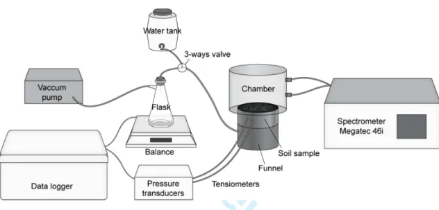
Fig. 1. Schematic overview of the multistep outflow system for hydric control and nitrous 565

oxide measurements. Intensity values corresponding to air and water are zoomed in (c) and 566

(d). 567

Fig. 2. Example of a gray scale slice with the segmented water and air, at the end of the

568

wetting phase and at the end of the drying phase. 569

Fig. 3. Evolution with time of the nitrous oxide fluxes and the matric potential measured by

570

the two tensiometers. Gray areas represent the drying phases, and white areas the wetting 571

phases. C1 is the first wetting-drying cycle, and C2 is the second wetting-drying cycle. 572

Fig. 4. Histograms of intensity values (16-bit), for (a) the first wetting-drying cycle, and (b)

573

the second wetting-drying cycle. Intensity values corresponding to air and water are zoomed 574

in (c) and (d). 575

Fig. 5. Three-dimensional distribution of the air phase (grey) and the water phase (blue) at the

576

end of the wetting phase and at the end of the drying phase for the two wetting-drying cycles. 577

Fig. 6. Evolution with time of (a) the air-filled and water-filled pore volume, and (b) the Euler

578

number of the total pore volume, (c) the air-filled pore volume, and (d) the Euler number of 579

the pores connected to the soil surface, for the first and second wetting-drying cycles. The 580

zero reference time is the beginning of the drying phase. 581

Fig. 7. Evolution with time of the relative gas diffusion coefficient of a 3-cm-thick subsample,

582

for the first and second wetting-drying cycles. The zero reference time is the beginning of the 583

drying phase. 584

For Review Only

585

Table 1. Pearson correlation matrix of the indicators extracted from the segmented X-ray images. 586 Variables Euler number (T) Euler number (S) Air volume (T) Air volume (S) Water volume (T) Gas diffusion coefficient (T) Euler number (T) 1.00 Euler number (S) 0.44 1.00 Air volume (T) ‒0.67 ‒0.91 1.00 Air volume (S) ‒0.72 ‒0.86 0.99 1.00 Water volume (T) 0.65 0.77 ‒0.94 ‒0.95 1.00 Gas diffusion coefficient (T) 0.01 ‒0.12 0.23 0.24 ‒0.41 1.00

T, calculated on the total air-filled pores identified; S, calculated on the air-filled pores connected to the soil surface.

For Review Only

Fig. 1. Schematic overview of the multistep outflow system for hydric control and nitrous oxide measurements.

For Review Only

Fig. 2. Example of a gray scale slice with the segmented water and air, at the end of the wetting phase and at the end of the drying phase.

For Review Only

Fig. 3. Evolution with time of the nitrous oxide fluxes and the matric potential measured by the two tensiometers. Gray areas represent the drying phases, and white areas the wetting phases. C1 is the first wetting-drying cycle, and C2 is the second wetting-drying cycle.

For Review Only

Fig. 4. Histograms of intensity values (16-bit), for (a) the first wetting-drying cycle, and (b) the second wetting-drying cycle. Intensity values corresponding to air and water are zoomed in (c) and (d).

For Review Only

Fig. 5. Three-dimensional distribution of the air phase (grey) and the water phase (blue) at the end of the wetting phase and at the end of the drying phase for the two wetting-drying cycles.

For Review Only

Fig. 6. Evolution with time of (a) the air-filled and water-filled pore volume, and (b) the Euler number of the total pore volume, (c) the air-filled pore volume, and (d) the Euler number of the pores connected to the soil surface, for the first and second wetting-drying cycles. The zero reference time is the beginning of the drying phase.

For Review Only

Fig. 7. Evolution with time of the relative gas diffusion coefficient of a 3-cm-thick subsample, for the first and second wetting-drying cycles. The zero reference time is the beginning of the drying phase.