HAL Id: halshs-00389690
https://halshs.archives-ouvertes.fr/halshs-00389690
Submitted on 29 May 2009
HAL is a multi-disciplinary open access
archive for the deposit and dissemination of
sci-entific research documents, whether they are
pub-lished or not. The documents may come from
teaching and research institutions in France or
abroad, or from public or private research centers.
L’archive ouverte pluridisciplinaire HAL, est
destinée au dépôt et à la diffusion de documents
scientifiques de niveau recherche, publiés ou non,
émanant des établissements d’enseignement et de
recherche français ou étrangers, des laboratoires
publics ou privés.
Imperfections
Nicolas Dromel
To cite this version:
Nicolas Dromel.
Stabilizing Fiscal Policies with Capital Market Imperfections.
2009.
�halshs-00389690�
Centre d’Economie de la Sorbonne
Stabilizing Fiscal Policies with Capital
Market Imperfections
Nicolas D
ROMELwith Capital Market Imperfections
∗
Nicolas L. Dromel
†May 12, 2009
∗ The author thanks Jean-Michel Grandmont and Patrick Pintus for insightful comments. Special thanks are also due to, without
implicating, Philippe Aghion, Stefano Bosi, Raouf Boucekkine, Pierre Cahuc, David de la Croix, Gabriel Desgranges, Rodolphe Dos Santos Ferreira, Fr´ed´eric Dufourt, Cecilia Garc´ıa-Pe˜nalosa, Guy Laroque, Etienne Lehmann, Francesco Magris, Franck Portier, Jos´e-V´ıctor R´ıos-Rull, Thomas Seegmuller; seminar and conference participants at various places for helpful discussions. The usual disclaimer applies.
† CNRS, Paris School of Economics, Centre d’Economie de la Sorbonne. Address correspondence to: Universit´e Paris 1 - MSE, 106-112
Abstract
We analyze how investment subsidies can affect aggregate volatility and growth in economies subject to capital market imper-fections. Within a model featuring both frictions on the credit market and unequal access to investment opportunities among individuals, we provide specific fiscal parameters able to reduce the probability of recessions, fuel the economy long-run growth rate and place it on a permanent-boom dynamic path. We analyze how conditions on the stabilizing fiscal parameters are modified when frictions in the economy evolve. Eventually, we show how this tax and transfer system can moderate persistence in the economy’s response to temporary and permanent productivity shocks.
Keywords: Endogenous Business Cycles; Capital Market Imperfections; Access to Productive Investment; Fiscal Policy;
Macroeconomic Stabilization.
R´esum´e
Ce papier analyse la fa¸con dont les subventions aux investissements peuvent affecter la volatilit´e et la croissance dans une ´economie sujette `a des imperfections sur le march´e du capital. Dans un mod`ele pr´esentant `a la fois des frictions sur le march´e du cr´edit et une in´egalit´e d’acc`es aux opportunit´es d’investissement, nous proposons des valeurs particuli`eres de param`etres fiscaux pouvant diminuer la probabilit´e d’occurrence de r´ecessions, renforcer la croissance `a long-terme et placer l’´economie sur un chemin d’expansion permanente. Nous analysons comment les param`etres de la politique fiscale stabilisatrice sont affect´es lorsque le niveau des frictions dans l’´economie varie. Enfin, nous montrons comment ce syst`eme fiscal peut mod´erer la persistance dans la r´eponse de l’´economie `a des chocs de productivit´e permanents et transitoires.
Mots-cl´es: Cycles d’Affaires Endog`enes ; Imperfections sur le March´e du Capital ; Acc`es `a l’Investissement Productif ; Politique
Fiscale ; Stabilisation Macro´economique.
1
Introduction
The growth and amplification effects of capital market frictions have been the subject of a large literature. At the aggregate level, a number of studies have highlighted the importance of credit constraints in explaining fluctuations in activity (see, in particular, Bernanke [11], Eckstein and Sinai [19], and Friedman [26]). Bernanke and Gertler [12] develop a business cycle model in which output dynamics are influenced by the situation of borrowers’ balance sheets. When the borrower net worth improves, agency costs of financing real capital investments are lowered. Net worth increases during booms, which entails smaller agency costs, rises investment, and amplifies the upturn (vice versa, during slumps). Fluctuations can therefore be initiated through shocks affecting net worth. In a dynamic economy where lenders cannot force borrowers to repay their debts unless the debts are secured, Kiyotaki and Moore [39] show that the interplay between credit limits and asset prices turns out to be a powerful transmission mechanism by which the effects of shocks persist, amplify, and spill over to other sectors. In their framework, small and non-permanent shocks to technology or income distribution can trigger large, persistent fluctuations in output and asset prices. In a dynamic general equilibrium model intended to further clarify the role of credit market frictions in business fluctuations, both from a qualitative and a quantitative standpoint, Bernanke, Gertler and Gilchrist [14] analyze the existence of a ”financial accelerator”. Typically, endogenous developments in credit markets would work to amplify and propagate shocks to the aggregate economy. Lags in investment can generate both hump-shaped output dynamics and a lead-lag relation between investment and asset prices, consistently with the empirical evidence. Also, firm heterogeneity can characterize a situation in which borrowers have differential access to capital markets.
The purpose of this paper is to analyze how investment subsidies can affect aggregate volatility and growth in economies subject to capital market imperfections. The model is based upon Aghion, Banerjee and Piketty [3] in which we introduce fiscal policy. In this setup, the coexistence of frictions on the capital market and inequality in the access to productive-investment opportunities can generate endogenous and permanent fluctuations in aggregate output, interest rates and investment. Savers and investors are separated along two dimensions. The first degree of separation is purely and simply physical: many agents who save are not able to invest directly in physical capital. As a matter of fact, skills, ideas and connections are necessary to invest in production. Furthermore, distances (geographic or social) may constitute an important barrier to investment. Indeed, public regulations may also restrict the access to investment. The second aspect of separation is characterized by a market failure: there exists a limit on the amounts investors
can borrow from savers. When the credit market development is high enough, and the separation between savers and investors is low enough, the economy can stay in a permanent-boom regime. In contrast, a high degree of such separation leads the economy to fluctuate around its steady-state growth path. When the credit market frictions are extremely tough, the economy falls into a permanent-slump regime. In a nutshell, economies displaying poorly developed financial markets and a strong physical separation between savers and investors will experience more volatility, and grow at a slower pace.
The contribution of the paper is to show that, under credit constraints, appropriate fiscal policy parameters are able to rule out the occurrence of slump regimes, and immunize the economy against endogenous cycles. For given levels of the credit market development, we provide specific fiscal parameters able to insulate the economy from recessions, fuel its long-run growth rate and place it on a permanent-boom dynamic path. The main mechanism driving our result is the following. The fiscal policy we analyze, introducing a tax on agents’ labor income and transferring the proceeds into investors’ wealth, is tantamount in dynamic terms to an increase in the fraction of the labor force having direct access to capital investment opportunities. More precisely, a structural policy that would remove institutional obstacles and rigidities separating savers and investors to promote growth, stability and equity at the same time, would presumably have a similar effect on the economy’s dynamics. We analyze how the conditions on the stabilizing fiscal parameters are modified when frictions in the economy evolve. Eventually, we study how the tax and transfer system impacts the response of the economy to temporary and permanent productivity shocks. Typically, aside from its direct growth-enhancing effects, it is shown that this type of fiscal policy moderates the persistence in the economy’s response to a shock (wealth distribution effects following a productivity shock in a slump episode are dampened).
Our findings complement the conclusions of Aghion et al. [3], who suggest that a government could absorb idle savings in the economy by public debt issuance. In many actual economies, the public debt option is often a constrained policy tool, and raises long-run issues regarding public finance sustainability and debt service credibility. In contrast, labor income taxation is a feature shared by all modern economies. Another dimension in which our paper departs from Aghion et al. [3] is that we provide an exhaustive analytic characterization of dynamic regimes possibilities, depending both on the fiscal parameters and friction levels.
The remainder of this paper proceeds as follows. Section 2 lays out the model, while section 3 analyzes dynamics and regime change conditions, showing how fiscal policy may help getting out of slumps, cycles, and fuel the growth rate.
Section 4 discusses the comparative statics properties of the suggested stabilizing and growth-enhancing fiscal policy. Section 5 investigates how this policy changes the response of the economy to productivity shocks. Some concluding remarks and directions for further research are gathered in section 6.
2
The Economy
This paper introduces fiscal policy, through labor income taxation and lump-sum transfers, into the positive long-run growth AK model with capital market imperfections studied in Aghion et al. [3]. For ease of comparison with this benchmark model, we keep the same notations and dynamic analysis methods.
2.1
Production
An homogeneous good is produced and serves both as capital and as a consumption commodity. In each period t ∈ N, agents are endowed with one unit of labor.
The good is produced according to the technology: F (K, L) = AKβL1−β = Y . We assume the growth rate of the
workforce to be at least equal to the one of the capital stock. Then, all agents are willing to work at a wage greater than or equal to one, so that the equilibrium labor price can be set to unity.
Assumption 2.1. ∂F
∂L = 1 ⇒ L = ¡
(1 − β)A¢1/βK ⇒ Y = σK with σ = A¡(1 − β)A)(1−β)/β
Positive long-run growth can be generated from this AK type setting. The parameter β stands for the capital share in final output, whereas (1 − β) denotes the labor share.
2.2
Dualism
The economy is physically split into two categories of agents. Only a fraction 0 ≤ µ ≤ 1 of the workforce (called the productive investors) can directly invest in physical capital. The other individuals (called the savers), can either
lend their savings to the productive investors at current interest rate r, or invest in a low-yield asset with a return
σ2< σ1= βσ. When µ increases from 0 to 1, the separation between savers and investors becomes thinner.
Due to asymmetric information issues (moral hazard) and incentive compatibility consideration, capital market is subject to a borrowing constraint. There is a constant 0 ≤ ν ≤ 1 such that anyone who wants to invest an amount I must have assets of at least νI. In other words, 1/ν is nothing else than a credit multiplier. Indeed, when ν decreases from 1 to 0, credit market development improves.
2.3
Interest rate setting
The AK type technology used in this framework implies that the equilibrium interest rate will take two possible values. When investment exceeds savings (i.e., demand for savings is (very) large), the gross interest rate will take its ”high” value σ1= βσ. In contrast, when savings are in excess supply, the gross equilibrium interest rate will drop to σ2< σ1.
2.4
Government
The government chooses tax policy and balances the budget at each point in time. The public authority is assumed to care about the level of productive investment in the economy. To this end, linear taxes are applied on agents’ labor income, to finance a transfer than can be thought of as an investment subsidy.
2.5
Timing
In the beginning of a period (say, in the morning), the respective amounts of planned investment and available savings in the economy are compared. Depending on their relative magnitude, the interest rate is set. If investment runs ahead of savings, the higher interest rate prevails, and the non-investors are willing to lend all their savings to the productive investors. Thus, during these boom episodes, all available savings in the economy will be invested in the high-yield activity. In contrast, if investment plans are not large enough to absorb all available savings, the interest rate will be set at its low value σ2. Then savers will be indifferent between issuing low-return loans, or investing in the low-yield
paid. Taxes are also levied and income transfers occur. Consumption finally takes place, from the net resources of the day. For sake of simplicity, and to ease comparisons with the Aghion et al. [3] benchmark model, a linear savings rate is assumed, as in the case of a standard logarithmic utility function. Both types of agents save a share (1 − α) of their wealth at the end of the day.1 The non-consumed part of the day’s net resources constitutes the amount of available
savings in the next morning.
2.6
Wealth Accumulation
Let Wt
B and WLt respectively represent the wealth levels of the borrowers (productive investors) and of the lenders (savers) in the morning of period (t + 1). We denote by St the total amount of savings: St = Wt
B + WLt, and
Id
t+1= WBt/ν the total planned investment in the morning of period (t + 1).
In a boom, the investment capacity of investors is higher than the available amount of savings ((Id
t+1 ≥ St). The prevailing interest rate is σ1 = βσ, such that all aggregate savings (WBt + WLt) are invested in the high-yield activity. The wealth accumulation of borrowers and lenders can be summarized as follows:
BOOM WBt+1= (1 − α)£(1 − τ )µ(1 − β)σ(WBt + WLt) + βσ(WBt + WLt) − βσWLt+ Tt ¤ (1) Wt+1 L = (1 − α) £ (1 − τ )(1 − µ)(1 − β)σ(Wt B+ WLt) + βσWLt ¤ (2)
The total return of the high-yield activity σ(Wt
B+ WLt), is shared between labor income with a fraction (1 − β), and capital income. Productive investors (resp. savers) represent a fraction µ (resp. 1 − µ) of the total labor share in output. Only borrowers take advantage of the return βσ on physical capital investment, but have to refund and pay the high level interest rate on the amount they borrowed (the whole Wt
L, since at the high interest rate σ1= βσ,
investing in the low-yield asset is a dominated strategy for lenders). To support productive investment, the government operates a transfer of resources by taxing labor income at rate 0 < τ < 1 and reallocating the proceeds Ttin the form of an investment subsidy.
1Introducing different propensities to consume for savers and investors would complicate the model without losing the basic results (cf.
As public budget is balanced in each period:
Tt= [τ µ + τ (1 − µ)](1 − β)σ(Wt
B+ WLt) (3)
Hence, we can re-write the borrowers’ wealth motion equation in a boom as:
WBt+1= (1 − α)©[µ + τ (1 − µ)](1 − β)σ(WBt + WLt) + βσWBt ª
(4)
In a slump, the investment capacity of productive investors is lower than the level of aggregate savings (Id
t+1< St). The prevailing interest rate is then σ2 < βσ, such that only W
t B
ν can be invested in the high-yield activity, generating a total revenue equal to σWBt
ν . SLUMP WBt+1= (1 − α)£(1 − τ )µ(1 − β)σ1 νW t B+ βσ 1 νW t B− σ2(1 ν − 1)W t B+ Tt ¤ (5) Wt+1 L = (1 − α) £ (1 − τ )(1 − µ)(1 − β)σ1 νW t B+ σ2(1 ν − 1)W t B+ σ2(WLt− ( 1 ν − 1)W t B) ¤ (6)
The total revenue σWBt
ν remunerates labor up to a fraction (1 − β), with borrowers (resp. lenders) getting a share µ (resp. 1 − µ) of that wage income. Only the borrowers get the fraction β of the total revenue, remunerating physical capital investment. As productive investors have actually borrowed Wt
B/ν − WBt, they repay this amount to the lenders
with the interest σ2 prevailing in a slump period. Aside from this repayment, lenders get also the return σ2 from
investing the rest of their savings in the low-yield activity. Once again, the government operates a transfer of resources by taxing labor income and reallocating the proceeds in the form of an investment subsidy.
As the public budget is balanced, we can re-write the borrowers’ wealth motion equation in a slump as:
Wt+1 B = (1 − α) © [µ + τ (1 − µ)](1 − β)σ1 νW t B+ βσ 1 νW t B− σ2( 1 ν − 1)W t B ª (7)
Let us notice that, both during booms or slumps, borrower’s physical capital income could also be taxed (say, at rate τk). As a matter of fact, there would be no difference in eq. (4) or (7) because of the balanced budget assumption (cf. Appendix A). However, taxing lender’s financial capital income (say, at rate τf) would make little sense since it would completely discourage loans to productive investors. As mentioned earlier, during slumps, the interest rate is at its low value σ2. After-tax rates of return on loans would then be equal to (1 − τf)σ2< σ2, and lending to borrowers
Besides, an interesting feature is that a proportional investment subsidy would have the same effect on dynamics as the lump-sum transfer to the borrowers we consider here (cf. Appendix A).
3
Analysis of the Dynamics
Defining qt= St Id t+1 = Wt B+WLt Wt
B ν as the ratio of aggregate savings over investment plans in the high-yield activity in the
morning of period (t + 1), we can obtain from the previous wealth motion laws the two following difference equations, allowing the global dynamics analysis of this economy.
When at the beginning of period t + 1 planned investment runs ahead of savings (qt≤ 1), the economy is in a boom:
1 qt+1 = [µ + τ (1 − µ)](1 − β) ν + β qt (BB)
In contrast, when qt> 1 the economy is experiencing a slump:
qt+1= £ (σ − σ2) + σ2qt ¤ [µ + τ (1 − µ)](1 − β)(σ/ν) + βσ/ν −¡(1/ν) − 1)σ2 (SS)
It is worth noticing that if we set τ to zero, we recover the benchmark model of Aghion et al. [3].
These two difference equations behavior can be studied graphically in the (qt, qt+1) plane. It is straightforward to show (cf. Appendix B) that (BB) is monotonic, increasing and concave while (SS) is linearly increasing. There are only three dynamic regimes the economy can actually experience, corresponding to the three possible rankings between 1,
b and s, where s and b are steady-state values of the savings to planned investment ratio, respectively determined by
the intersections between (SS) and (BB) with the 450 line. When qt≤ 1 (i.e., when the planned investment volume is higher than the aggregate savings amount), only the (BB) curve is relevant, while if qt> 1, only the (SS) locus prevails.
The steady-state savings to planned investment ratio in a boom writes as b = ν
µ+τ (1−µ). As soon as b ≤ 1, the economy is in a permanent boom.
From any initial qt < 1, the economy will converge to b, and the long-run growth rate is nothing else than the Harrod-Domar one, that is the product of the savings rate by the average productivity of capital g∗ = (1 − α)σ (cf. Appendix C). The condition for a permanent boom can also be written in terms of the fiscal parameter τ : the economy will experience a permanent boom regime if and only if
τ ≥ν − µ
1 − µ = τb
Increasing τ lowers the level of (BB) in the plane and the savings to planned investment steady-state level b. The ordinate to origin of (BB) qt+1|
qt=0= 0 remains equal to zero, whatever the tax rate.
The steady-state savings to planned investment ratio in a slump writes as s = (σ−σ2)ν
[µ+τ (1−µ)](1−β)σ+βσ−σ2. As soon as
s > 1, the economy will go through a permanent slump.
— Figure 2 about here —
The condition for the permanent slump can be also stated as function of the fiscal parameter τ :
τ < ν(σ − σ2) + σ2− βσ − µ(1 − β)σ
(1 − β)σ(1 − µ) = τs
Increasing τ lowers the level of (SS) in the plane and the steady-state savings to planned investment ratio s. The ordinate to origin of (SS) drops when the tax rate is increased since ∂
∂τ(qt+1|qt=0) < 0. The long-run growth rate in a slump can be written as gs= (1−α)ν {[µ + τ (1 − µ)](1 − β)σ + βσ − σ2(1 − ν)} = (1 − α){σs + (1 −1s)σ2}, and clearly
depends positively on the fiscal parameter τ . Since, b − s = ν(βσ−σ2)(1−τ )(1−µ)
[µ+τ (1−µ)]{[µ+τ (1−µ)](1−β)σ+βσ−σ2} > 0, we know that b is
always greater than s. However, the distance between the two steady-state savings to planned investment ratios shrinks as soon as τ increases from 0 to 1.
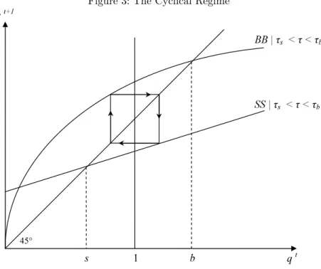
The remaining case corresponds to the intermediary situation where τs< τ < τb. In that situation, a cyclical regime prevails.
— Figure 3 about here —
cycle, which periodicity depends upon some deep parameters of the model. The intuition behind the cyclical motion is the following. During episodes of slow growth, savings are abundant with respect to the limited debt capacity of potential investors, which generates a low demand for savings and low equilibrium interest rates. Hence, investors can keep a large fraction of their profits (since the the debt burden is low), which allows them to rebuild reserves, debt capacity and increase investment. This in turn, entails more profits and investment until, eventually, planned investment exceeds savings and interest rates go up. The debt burden will then be larger, retained profit smaller, investment will drop, and growth will be slower.2
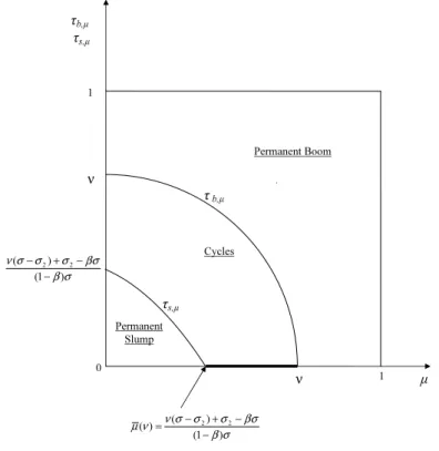
We can summarize the different dynamic regimes by the following proposition: Proposition 3.1 (Stabilizing and Growth-Enhancing Fiscal Policy).
1. When ν < µ, the economy is in a permanent boom whatever τ . This case is covered in Aghion et al. [3]
2. When µ < ν, the economy
1. is in a permanent boom if τ > ν−µ1−µ = τb ⇔ b < 1
2. is in a permanent slump if τ < ν(σ−σ2)+σ2−βσ−µ(1−β)σ
(1−β)σ(1−µ) = τs⇔ s > 1.
3. cycles if τs< τ < τb⇔ s < 1 < b.
Let ν = ¯ν(µ) = µ(1−β)σ+βσ−σ2
σ−σ2 ⇔ τs= 0. We will have τb> 0 ⇔ ν > µ and τs> 0 ⇔ ν > ¯ν(µ).
• For any µ < ν < ¯ν(µ) : if 0 < τ < τb then the economy experiences a cyclical regime, alternating between phases
of expansion and downturns; if τb < τ , the economy is in a permanent boom, which long-run growth rate is the
Harrod-Domar one.
• For any ¯ν(ν) < ν < 1 : if 0 < τ < τs, the economy is trapped into a permanent-slump regime; if τs< τ < τb then
the economy experiences a cyclical regime alternating between phases of expansion and downturns; if τb< τ , the
economy is in a permanent boom, which long-run growth rate is the Harrod-Domar one.
2Allowing instead the productive investors to choose among a continuum of technologies would give a continuum of equilibrium interest
rates values. Let us stress that in such a situation, as discussed in Aghion et al. [3], aggregate cycles could still be obtained. Therefore, the assumption of an equilibrium interest rate moving discontinuously from a high to a low value (and vice versa) does not seem responsible for the emergence of endogenous fluctuations.
Similarly, one can get related results by analyzing the dynamics regimes for fixed values of µ (cf. Appendix D)
If the tax rate initially set to τ < τs is raised to a value τs < τ0 < τb, the dynamic regime goes from a permanent slump to a cyclical motion (cf. Fig. 4). Starting from the previous permanent slump steady-state level of the savings to planned investment ratio, the economy hits the new (SS’) locus, and enters a cycle, alternating between temporary booms and slumps.
— Figure 4 about here —
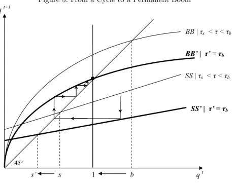
If the tax rate initially set to τs< τ < τb is raised to a value τ0 = τb, the dynamic regime goes from a cycle to a permanent boom (cf. Fig. 5). In that case, b is set equal to 1, so that the economy can not go back to the slump zone, since when q ≤ 1, only (BB) is relevant.
— Figure 5 about here —
Eventually, if the tax rate initially set to τ < τs is raised to a value τ0 = τb, the dynamic regime goes from a permanent slump to a permanent boom (cf. Fig. 6). In that case, b is set equal to 1, so that the economy can not go back to the slump zone, since when q ≤ 1, only (BB) is relevant.
— Figure 6 about here —
3.1
Intuition
To gain insight into the mechanism that drives our result, it is useful to analyze how the introduction of this fiscal scheme affects the fractions of the labor share going respectively to investors and to savers. Actually, introducing a tax on savers’ labor income and transferring the proceeds into the investors’ wealth is tantamount to an increase in the fraction of the labor force having direct access to capital investment opportunities. As a matter of fact, the original
setup studied in Aghion et al. [3] is modified up to the following parameter changes : µ becomes µ + (1 − µ)τ , which is increasing in τ , and (1 − µ) becomes (1 − µ)(1 − τ ), which is decreasing in τ .
In other words fiscal policy, usually mobilized as a conventional countercyclical tool, affects here the economy in the same way as a structural reform would do. More precisely, a structural policy that would eliminate institutional barriers and rigidities separating savers and investors to foster growth, stability and equity, would presumably have a similar effect on the economy dynamics. In general, such structural policies may be difficult to implement, and are in some cases just not attainable: authorities cannot simply choose that access to credit and investment opportunities should be enhanced. Interestingly, with a very basic setup, the fiscal policy we feature can impact the dynamics as if a structural policy had managed to improve the access to productive investment opportunities.
4
Comparative Statics
In the following section, we assess how τb and τsbehave when one of the friction parameters ν and µ is made to vary (cf. Appendix E for detailed expressions).
4.1
Comparative Statics Properties of τ
band τ
swith respect to ν
Let τb,ν and τs,ν be the geometrical loci respectively depicting the sensitivity of τb and τs with respect to ν, caeteris
paribus.
— Figure 7 about here —
τb,ν and τs,ν are linear. Since 0 < ∂τ∂νb < ∂τ∂νs, both are upward sloping, but τs,ν is steeper than τb,ν. It can be easily shown that 0 < µ = ν|τb=0 < ν|τs=0 = ¯ν(µ) < 1, so that τs,ν hits the abscissa axis for a higher value of ν than τb,ν
does. As τb− τs> 0, τb,ν is always ”higher” than τs,ν in the plane, for any value of ν > µ . The intersection of τb,ν and
Let us now turn to the effect of a variation in µ (i.e., a change in the access to productive investment opportunities) on the respective properties of τb,ν and τs,ν. We suppose µ goes from µ1to µ2> µ1, i.e. the separation between savers
and productive investors is smaller.
— Figure 8 about here —
Since 0 < ∂2τb
∂µ∂ν < ∂2τ
s
∂µ∂ν, when µ increases, both τb,ν and τs,ν become steeper, but the steepness rise is higher for
τs,ν. Moreover, as 0 < ∂µ∂ ¯ν(µ) < ∂µ∂ (ν|τb=0) = 1, both abscissa to origin values of τb,ν and τs,ν increase following a
rise in µ, but the abscissa to origin value of τb,ν reacts more. Hence, when the degree of separation between savers and investors decreases (µ goes up from µ1 to µ2), the permanent-boom likelihood is increased for any ν ≥ µ1(permanent
boom can be achieved with a lower τ ) and the permanent-slump likelihood reduces for any ν ≥ ¯ν(µ1) (we can get
out of slumps with a lower τ ). The cycles likelihood reduces for any µ1< ν < ¯ν(µ1) and expands for any ν > ¯ν(µ1).
We also notice that ∂
∂µ(τb− τs) > 0. Very intuitively, improving the access to investment opportunities facilitates the conditions needed to reach a permanent boom, or to get out from a permanent-slump trap.
Besides, τb,ν and τs,ν can also be affected by a productivity shock (namely, a rise in σ, from σ1 to σ2> σ1). Since
0 = ∂2τ b ∂σ∂ν < ∂ 2τ s ∂σ∂ν and 0 = ∂σ∂ (ν|τb=0) < ∂
∂σν(µ), both the slope and the abscissa to origin value of τ¯ s,ν will go up,
whereas τb,ν will remain unchanged. Hence, if a productivity shock occurs, the likelihood of permanent booms will remain unchanged for any 0 < ν < 1, while the permanent-slump likelihood will reduce and the cycles likelihood will increase for any ν > ¯ν(µ)|σ=σ1.
4.2
Comparative Statics Properties of τ
band τ
swith respect to µ
Let τb,µ and τs,µ be the geometrical loci respectively depicting the sensitivity of τb and τs with respect to µ, caeteris
paribus.
Since ∂τs ∂µ < ∂τb ∂µ < 0 and ∂2τ s ∂µ2 < ∂ 2τ b
∂µ2 < 0, both τb,µ and τs,µ are decreasing and concave, but τs,µ is more concave.
The ordinate and abscissa to origin values of τb,µ are the same. The locus τs,µ shares the same property, such that: 0 < τs|µ=0 = µ|τs=0= ¯µ(ν) < µ|τb=0= τb|µ=0= ν < 1.
Let us now turn to the effect of a variation in ν, (i.e. a change in the credit market development), on the properties of τb,µ and τs,µ. We suppose ν goes from ν1 to ν2> ν1, i.e. the credit market development gets poorer.
— Figure 10 about here —
Since 0 < ∂2τ b ∂ν∂µ < ∂ 2τ s ∂ν∂µ, and 0 < ∂ν∂ (µ|τb=0) = ∂
∂ν(τb|µ=0) < ∂ν∂ (τs|µ=0) = ∂ν∂ µ(ν), the upward shift and the¯ concavity reduction of τs,µ following a rise in ν is stronger than the reaction of τb,µ. Hence, when conditions on the credit market deteriorate (ν increases from ν1 to ν2), the permanent-slump likelihood increases for any 0 < µ < ¯µ(ν2)
(we need a higher τ to get out from the permanent slump) and the permanent-boom likelihood decreases for any 0 < µ < ν2. The cycles likelihood reduces for any 0 < µ < ¯µ(ν2), but increases for any ¯µ(ν2) < µ < ν2. We also notice
that ∂
∂ν(τb− τs) < 0. Very intuitively, a deterioration in the credit market development makes stronger the conditions needed to reach a permanent boom, or to get out from a permanent slump.
Besides, τb,µ and τs,µ can also be affected following a productivity shock (namely, a rise in σ from σ1 to σ2> σ1).
Since ∂2τs ∂σ∂µ < ∂2τ b ∂σ∂µ = 0 and ∂σ∂ µ(ν) =¯ ∂σ∂ (τs|µ=0) < ∂σ∂ (µ|τb=0) = ∂
∂σ(τb|µ=0) = 0, we know that both the slope, the abscissa to origin and the ordinate to origin values of τs,µ will decrease following a productivity shock, whereas τb,µwill remain unchanged. Hence, for any µ < ¯µ(ν)|σ=σ1 the likelihood of permanent slumps will reduce and the likelihood of
cycles will increase. However, the likelihood of permanent boom will remain unchanged for any 0 < µ < 1.
5
Response to Shocks
Is the fiscal structure featured in this economy able to affect its reaction to productivity shocks (such as shocks on σ)? As in the benchmark case of Aghion et al. [3], σ does not appear in the expression of (BB). It can be easily shown in a boom that, following a shock on σ (may it be permanent or temporary), loans repayments and investment returns
vary in the exact same proportion, so that the distribution of wealth between savers and investors remains unchanged (indeed, q provides a direct measure of any evolution in this repartition). A productivity shock during a boom does affect the Harrod-Domar growth rate g∗. But as q is not affected by any variation in the productivity level, all the shock will be registered instantly in g∗ (there will be no indirect effects due to a change in wealth distribution). Put differently, the tax schedule has no effect whatsoever on the way g∗ reacts to σ.
In contrast, during slumps, (SS) does react to any variation in σ (Cf. Appendix C and Appendix F). Since∂∂σ∂q2qt+1t < 0
a positive productivity shock on σ decreases the slope of the (SS) curve. We can see from ∂τ ∂σ∂q∂3qt+1t > 0 that increasing
τ makes ∂∂σ∂q2qt+1t less negative. In other words, the reduction in the slope of (SS) due to a productivity shock is lower
when the tax rate is high. Moreover, following a productivity shock, the ordinate to origin of (SS) goes up since, ∂
∂σ(qt+1|qt=0) > 0. Increasing τ moderates this increase, as ∂τ∂ [∂σ∂ (qt+1|qt=0)] < 0.
— Figure 11 about here —
Following a permanent productivity shock (cf. Fig. 11), the steady-state savings to planned investment ratio in a slump s decreases, since ∂s
∂σ < 0. Hence, aside from the direct effect of σ on gs,
∂gs
∂σ > 0, the drop in s adds an indirect
effect on growth, via the shift in wealth distribution in favor of the productive investors as q goes down. However, when the tax rate is increased, s still decreases following a productivity shock, but to a lower extent, since: ∂2s
∂τ ∂σ > 0. Hence, although ∂2gs
∂τ ∂σ > 0 which basically says that τ reinforces the direct positive effect on gs of a positive shock on
σ, the indirect growth effects linked to the convergence to the new steady state will be smaller when taxes (and thus
subsidies) are increased. In other words, this type of fiscal policy moderates persistence in the economy’s response to a shock.
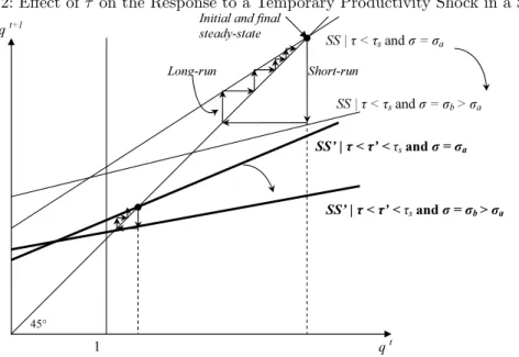
When the productivity shock is only temporary (cf. Fig. 12), the steady-state savings to planned investment ratio does not change. When τ is increased, both the short-run and the long-run convergence path will be shorter, also meaning weaker indirect wealth distribution effects and smaller persistence.
6
Conclusion
The purpose of this paper is to analyze how investment subsidies can affect aggregate volatility and growth in economies subject to capital market imperfections. Within a model featuring both frictions on the credit market and unequal access to investment opportunities among individuals, we have shown that appropriate fiscal policy parameters are able to rule out the occurrence of slump regimes, and immunize the economy against endogenous fluctuations in GDP, investment and interest rates. For given levels of the credit market development, we provide specific fiscal parameters able to insulate the economy from recessions, fuel its long-run growth rate and place it on a permanent-boom dynamic path.
The main mechanism driving our result is the following. The fiscal policy we consider, introducing a tax on agents’ labor income and transferring the proceeds into the investors’ wealth, is tantamount to a decrease in the fraction of agents unable to invest directly in the production process. We analyze how conditions on the stabilizing fiscal parameters are modified when frictions in the economy evolve. Eventually, we study how the tax and transfer system impacts the economy’s response to temporary and permanent productivity shocks. Typically, aside from its direct growth-enhancing effects, it is shown that this type of fiscal policy moderates the persistence in the economy’s response to a shock (wealth distribution effects following a productivity shock in a slump episode are dampened).
These findings complement the conclusions of Aghion et al. [3]. Abstracting from public debt issuance, which can be a constrained instrument in many modern economies and raises long-run issues regarding public finance sustainability, we show that investment subsidies financed through labor income taxation has stabilizing properties in economies where capital markets are subject to frictions. Moreover, we provide an exhaustive analytic characterization of dynamic regimes possibilities, depending both on the fiscal parameters and friction levels.
Some directions for further research naturally follow. An analysis of ”optimal fiscal rules”, aimed at achieving both stabilization and inequality reduction in this economy would certainly be of interest. Moreover, allowing for heterogeneity in the investment projects would be useful for understanding how credit market imperfections affect the macroeconomy through the composition of the credit. We plan to pursue these projects in the near future.
Appendix
A
Alternative Fiscal Structures
A.1
Adding capital income taxation for borrowers
If borrowers were also to pay capital income taxes, we would rigorously obtain the same reduced-form wealth accumu-lation equations as in the case with labor income taxes only, due to the balanced public budget assumption.
For instance in a boom:
Wt+1 B = (1 − α) £ (1 − τ )µ(1 − β)σ(Wt B+ WLt) + (1 − τk)βσ(WBt + WLt) − βσWLt + Tt ¤ (8) Wt+1 L = (1 − α) £ (1 − τ )(1 − µ)(1 − β)σ(Wt B+ WLt) + βσWLt ¤ (9)
As public budget is balanced in each period:
Tt= {[τ µ + τ (1 − µ)](1 − β) + τkβ}σ(Wt
B+ WLt) (10)
Hence, we can re-write the borrowers’ wealth motion equation in a boom as:
WBt+1= (1 − α)©[µ + τ (1 − µ)](1 − β)σ(WBt + WLt) + βσWBt ª
(11) which is identical to eq. (4).
On the other hand, during a slump:
Wt+1 B = (1 − α) £ (1 − τ )µ(1 − β)σ1 νW t B+ (1 − τk)βσ 1 νW t B− σ2(1 ν − 1)W t B+ Tt ¤ (12) Wt+1 L = (1 − α) £ (1 − τ )(1 − µ)(1 − β)σ1 νW t B+ σ2(1 ν − 1)W t B+ σ2(WLt− ( 1 ν − 1)W t B) ¤ (13)
As public budget is balanced, we can re-write the borrowers’ wealth motion equation in a slump as:
Wt+1 B = (1 − α) © [µ + τ (1 − µ)](1 − β)σ1 νW t B+ βσ 1 νW t B− σ2(1 ν − 1)W t B ª (14) which is identical to eq. (7).
A.2
Proportional rather than lump-sum investment subsidy
If the investment subsidy was granted in a proportional rather than a lump-sum way, we would also obtain the same reduced-form wealth accumulation equations.
For instance in a boom:
Wt+1 B = (1 − α) £ (1 − τ )µ(1 − β)σ(Wt B+ WLt) + βσ(WBt + WLt) − βσWLt ¤ (1 + γ) (15) Wt+1 L = (1 − α) £ (1 − τ )(1 − µ)(1 − β)σ(Wt B+ WLt) + βσWLt ¤ (16)
As public budget is balanced in each period: (1 − α)γ£(1 − τ )µ(1 − β)σ(Wt
B+ WLt) + βσ(WBt + WLt) − βσWLt ¤
= (1 − α)[τ µ + τ (1 − µ)](1 − β)σ(Wt
B+ WLt) (17)
Hence, we can re-write the borrowers’ wealth motion equation in a boom as:
WBt+1= (1 − α)£(1 − τ )µ(1 − β)σ(Wt B+ WLt) + βσ(WBt+ WLt) − βσWLt ¤ + (1 − α)[τ µ + τ (1 − µ)](1 − β)σ(Wt B+ WLt) (18) Wt+1 B = (1 − α) © [µ + τ (1 − µ)](1 − β)σ(Wt B+ WLt) + βσWBt ª (19) which is identical to eq. (4).
On the other hand, during a slump:
Wt+1 B = (1 − α) £ (1 − τ )µ(1 − β)σ1 νW t B+ βσ 1 νW t B− σ2(1 ν − 1)W t B ¤ (1 + γ) (20) Wt+1 L = (1 − α) £ (1 − τ )(1 − µ)(1 − β)σ1 νW t B+ σ2(1 ν − 1)W t B+ σ2(WLt− ( 1 ν − 1)W t B) ¤ (21)
As public budget is balanced, we can re-write the borrowers’ wealth motion equation in a slump as:
Wt+1 B = (1 − α) © [µ + τ (1 − µ)](1 − β)σ1 νW t B+ βσ 1 νW t B− σ2(1 ν − 1)W t B ª (22) which is identical to eq. (7).
B
Properties of the BB and SS loci
B.1
The BB locus
Since ∂q∂qt+1t = β [µ+τ (1−µ)](1−β)qtν+β > 0, and ∂2qt+1 ∂(qt)2 = − 2β(1−β)[µ+τ (1−µ)]ν{[µ+τ (1−µ)](1−β)qtν+β}3 < 0, (BB) is positively sloped and
concave.
Moreover when τ is increased, (BB) moves downwards: ∂∂τ ∂q2qt+1t = −
2β(1−β)(1−µ)qt
ν{[µ+τ (1−µ)](1−β)qt ν+β}3
< 0.
The steady-state level in a boom writes as: b = ν µ+τ (1−µ).
Since ∂b ∂τ = −
ν(1−µ)
[µ+τ (1−µ)]2 < 0, the steady-state level b decreases when τ increases.
The ordinate to origin qt+1|
qt=0= 0 remains zero, whatever the tax rate.
B.2
The SS locus
Since ∂q∂qt+1t = [µ+τ (1−µ)](1−β)σ+βσ−σσ2ν 2(1−ν) > 0, (SS) is linear and positively sloped.
The ordinate to origin of (SS) writes as qt+1|
qt=0= σ−σ2 [µ+τ (1−µ)](1−β)(σ/ν)+βσ/ν−¡1/ν−1)σ2 . Since ∂ ∂τqt+1|qt=0= − (σ−σ2)(1−µ)(1−β)σ ν{[µ+τ (1−µ)](1−β)(σ/ν)+βσ/ν−¡1/ν−1)σ2}2
< 0, increasing τ lowers the ordinate to origin.
Moreover, since ∂∂τ ∂q2qt+1t = −
σ2(1−µ)(1−β)σν
{[µ+τ (1−µ)](1−β)σ+βσ−σ2(1−ν)}2 < 0, increasing τ decreases the slope of (SS).
The steady-state level in a slump writes as: qt+1= qt= s = (σ−σ2)ν
[µ+τ (1−µ)](1−β)σ+βσ−σ2.
Since ∂s ∂τ = −
ν(σ−σ2)(1−µ)(1−β)σ
{[µ+τ (1−µ)](1−β)σ+βσ−σ2}2 < 0 the steady-state level s is lower when τ increases.
Nota: the (BB) curve always lies above the (SS) locus at qt= 1:
qt+1(qt= 1, rt+1= σ 1) = ½ [µ+τ (1−µ)](1−β) ν + β ¾−1 > qt+1(qt= 1, rt+1= σ 2) = ½ £ µ + τ ](1 − β)/ν¤+ (β/ν) −£(1/ν − 1)¤(σ2/σ) ¾−1
B.3
Steady state levels
Since b − s = ν(βσ−σ2)(1−τ )(1−µ)
[µ+τ (1−µ)]{[µ+τ (1−µ)](1−β)σ+βσ−σ2} > 0, we know that b is always greater than s.
Since ∂
∂τ(b − s) =
−ν(βσ−σ2)(1−µ)h[µ+τ (1−µ)](1−β)σ{2−[τ (1−µ)+µ]}+βσ−σ2i
[µ+τ (1−µ)]2{[µ+τ (1−µ)](1−β)σ+βσ−σ2}2] < 0, we know that increasing τ reduces the gap
between b and s, from (b − s)|τ =0= ν(βσ−σ2)(1−µ)
µ[µ(1−β)σ+βσ−σ2] > 0 to (b − s)|τ =1= 0.
C
Growth rates
In a boom Id
t+1≥ St, the actual investment in the high-yield activity is min(St, It+1d ) = St.
The boom growth rate can then be measured by: Yt+2
Yt+1 = σKt+2 σKt+1 = σSt+1 σSt = (1 − α)σ = g ∗. In a slump, Id
t+1< St, the actual investment in the high-yield activity is min(St, It+1d ) = It+1d .
The slump growth rate will be therefore written as: Kt+2
Kt+1 = Wt+1 B /ν Wt B/ν = (1−α) ν {[µ + τ (1 − µ)](1 − β)σ + βσ − σ2(1 − ν)} = gs= (1 − α){σs + (1 −1s)σ2}. Since ∂gs ∂τ = (1−α)
ν (1 − µ)(1 − β)σ > 0, raising τ increases long-run growth during slumps.
Indeed gs|τ =0=(1−α)ν [µ(1 − β)σ + βσ − σ2(1 − ν))] < gs|τ >0.
Very intuitively, a positive productivity shock on σ affects positively the growth rate, both during booms and during slumps: ∂g∂σ∗ = (1 − α) > 0 and ∂gs ∂σ = (1−α) ν {[µ + τ (1 − µ)](1 − β) + β} > 0. Since ∂2g s ∂τ ∂σ = (1−α) ν (1 − µ)(1 − β) > 0, we know that increasing τ reinforces the positive effect on gs of a positive shock on σ.
D
Proposition 3.1 Continued
One can get related results by analyzing the dynamics regimes for fixed values of µ:
µ = ¯µ(ν) = ν(σ−σ2)+σ2−βσ
• For any ¯µ(ν) < µ < ν : if 0 < τ < τbthen the economy experiences a cyclical regime, alternating between phases of expansion and downturns; if τb< τ , the economy is in a permanent boom, which long-run growth rate is the
Harrod-Domar one.
• For any 0 < µ < ¯µ(ν) : if 0 < τ < τs, the economy is trapped into a permanent-slump regime; if τs< τ < τb then
the economy experiences a cyclical regime alternating between phases of expansion and downturns; if τb< τ , the
economy is in a permanent boom, which long-run growth rate is the Harrod-Domar one.
Nota : ¯µ(ν) =[¯ν(µ)+ν](σ−σ2)−µ(1−β)σ−2(βσ−σ2)
(1−β)σ .
E
Comparative Statics (Detailed Expressions)
E.1
Comparative Statics Properties of τ
band τ
swith respect to ν
Let τb,ν and τs,ν be the geometrical loci respectively depicting the sensitivity of τb and τs with respect to ν, caeteris
paribus.
τb,ν and τs,ν are linear. Since 0 < (1−µ)1 = ∂τ∂νb < (1−β)σσ−σ2 ∂τ∂νb = ∂τ∂νs, both are upward sloping, but τs,ν is steeper than τb,ν. Since 0 < µ = ν|τb=0 < ν|τs=0 = ¯ν(µ) =
µ(1−β)σ+βσ−σ2
σ−σ2 < 1, τs,ν hits the abscissa axis for a higher value
of ν than τb,ν does. Since, τb− τs= (βσ−σ(1−β)σ(1−µ)2)(1−ν) > 0, τb,ν is always ”higher” than τs,ν in the plane, for any value of
ν >= ν|τb=0= µ . The intersection of τb,ν and τs,ν occurs at ν = 1.
Let us now turn to the effect of a variation in µ (i.e. a change in the access to productive investment opportunities) on the properties of τb,ν and τs,ν.We suppose µ goes from µ1 to µ2 > µ1, i.e. the separation between savers and
productive investors is smaller.
Since 0 < 1 (1−µ)2 = ∂ 2τ b ∂µ∂ν < (1−β)σσ−σ2 ∂ 2τ b ∂µ∂ν = ∂ 2τ s
∂µ∂ν, when µ increases, τb,ν and τs,ν become steeper, but the steepness rise is higher for τs,ν. Moreover as 0 < ∂
∂µν(µ) =¯ ∂µ∂ (ν|τs=0) =
(1−β)σ
σ−σ2 <
∂
∂µ(ν|τb=0) = 1, both abscissa to origin
values of τb,ν and τs,ν increase following a rise in µ, but abscissa to origin value of τb,ν reacts more. Hence, when the degree of separation between savers and investors decreases (µ goes up from µ1to µ2), the permanent-boom likelihood is
increased for any ν ≥ µ1(permanent boom can be achieved with a lower τ ) and the permanent-slump likelihood reduces
for any ν ≥ ¯ν(µ1) (we can get out of slumps with a lower τ ). The cycles likelihood reduces for any µ1 < ν < ¯ν(µ1)
and expands for any ν > ¯ν(µ1). We also notice that ∂µ∂ (τb− τs) = (βσ−σ(1−β)σ(1−µ)2)(1−ν)2 > 0. Very intuitively, improving the
access to investment opportunities facilitates the conditions needed to reach a permanent boom, or to get out from a permanent-slump trap.
Besides, τb,ν and τs,ν can also be affected by a productivity shock (namely, a rise in σ, from σ1 to σ2> σ1). Since
0 = ∂2τb ∂σ∂ν < ∂2τ s ∂σ∂ν = σ2 (1−β)σ2(1−µ) and 0 = ∂σ∂ (ν|τb=0) < ∂ ∂σ(ν|τs=0) = ∂ ∂σν(µ) =¯ σ2(1−β)(1−µ)
(σ−σ2)2 , both the slope and the
abscissa to origin value of τs,ν will go up, whereas τb,ν will remain unchanged. Hence, if a productivity shock occurs, the likelihood of permanent booms will remain unchanged for any 0 < ν < 1, while the permanent-slump likelihood reduces and the cycles likelihood increases for any ν > ¯ν(µ)|σ=σ1.
E.2
Comparative Statics Properties of τ
band τ
swith respect to µ
Let τb,µ and τs,µ be the geometrical loci respectively depicting the sensitivity of τb and τs with respect to µ, caeteris
paribus. Since ∂τs ∂µ = (1−β)σσ−σ2 ∂τ∂µb < ∂τ∂µb = −(1−µ)1−ν2 < 0 and ∂ 2τ s ∂µ2 = (1−β)σσ−σ2 ∂ 2τ b ∂µ2 < ∂ 2τ b ∂µ2 = − 2(1−ν)
(1−µ)3 < 0, both τb,µ and τs,µ are decreasing and concave, but τs,µ is more concave. The ordinate and abscissa to origin values of τb,µ are the same. The locus τs,µshares the same property, such that: 0 <ν(σ−σ2)+σ2−βσ
(1−β)σ = τs|µ=0 = µ|τs=0= ¯µ(ν) < µ|τb=0= τb|µ=0= ν < 1.
Let us now turn to the effect of a variation in ν, (i.e. a change in the credit market development), on the properties of τb,µ and τs,µ. We suppose ν goes from ν1 to ν2> ν1, i.e. the credit market development gets poorer.
Since 0 < 1 (1−µ)2 = ∂ 2τ b ∂ν∂µ < σ−σ2 (1−β)σ ∂2τ b ∂ν∂µ = ∂2τ s ∂ν∂µ, and 0 < 1 = ∂ν∂ (τb|µ=0) = ∂ν∂ (µ|τb=0) < ∂ ∂ν(τs|µ=0) = ∂ ∂ν(µ|τs=0) = ∂
∂νµ(ν) =¯ (1−β)σσ−σ2 , the upward shift and the concavity reduction of τs,µfollowing a rise in ν is stronger than the reaction
of τb,µ. Hence, when conditions on the credit market deteriorate (ν increases from ν1 to ν2), the permanent-slump
likelihood increases for any 0 < µ < ¯µ(ν2) (we need a higher τ to get out from the permanent slump) and the
permanent-boom likelihood decreases for any 0 < µ < ν2). The cycles likelihood reduces for any 0 < µ < ¯µ(ν2), but increases for
market development makes stronger the conditions needed to reach a permanent boom, or get out from a permanent slump.
Besides, τb,µ and τs,µ can also be affected following a productivity shock (namely, a rise in σ from σ1 to σ2> σ1).
Since − σ2(1−ν) (1−β)σ2(1−µ)2 = ∂ 2τ s ∂σ∂µ < ∂ 2τ b ∂σ∂µ = 0 and − σ2(1−ν) (1−β)σ2 = ∂σ∂ (µ|τs=0) = ∂ ∂σµ(ν) =¯ ∂σ∂ (τs|µ=0) < ∂σ∂ (µ|τb=0) = ∂
∂σ(τb|µ=0) = 0, both the slope, the abscissa to origin and the ordinate to origin values of τs,µ will decrease following a productivity shock, whereas τb,µ will remain unchanged. Hence, for any µ < ¯µ(ν)|σ=σ1 the likelihood of permanent
slumps will reduce and the likelihood of cycles will increase. However, the likelihood of permanent boom will remain unchanged for any 0 < µ < 1.
F
Response to Productivity Shocks during Slumps
Since ∂∂σ∂q2qt+1t =
−νσ2{[µ+τ (1−µ)](1−β)+β}
{[µ+τ (1−µ)](1−β)σ+βσ−σ2(1−ν)}2 < 0 a positive productivity shock on σ decreases the slope of the (SS)
curve. We can see from ∂τ ∂σ∂q∂3qt+1t =
νσ2(1−µ)(1−β){[µ+τ (1−µ)](1−β)σ+βσ+σ2(1−ν)}
{[µ+τ (1−µ)](1−β)σ+βσ−σ2(1−ν)}3 > 0 that increasing τ makes
∂2qt+1
∂σ∂qt less
negative. In other words, the reduction in the slope of (SS) due to a productivity shock is lower when the tax rate is high.
Moreover, following a productivity shock, the ordinate to origin of (SS) goes up since: ∂
∂σ(qt+1|qt=0) =
νσ2{[µ+τ (1−µ)](1−β)+β−(1−ν)}
{[µ+τ (1−µ)](1−β)σ+βσ−σ2(1−ν)}2 > 0. Increasing τ moderates this increase in the ordinate to origin,
since: ∂
∂τ[∂σ∂ (qt+1|qt=0)] =
νσ2(1−µ)(1−β)(σ2−2σ){[µ+τ (1−µ)](1−β)+β−(1−ν)}
{[µ+τ (1−µ)](1−β)σ+βσ−σ2(1−ν)}3 < 0.
Following a productivity shock, the steady-state level in a slump s decreases, since ∂s ∂σ =
−νσ(1−β)(1−µ)(1−τ ) {[µ+τ (1−µ)](1−β)σ+βσ−σ2}2 <
0. However, when the tax is increased, s still decreases following a productivity shock, but in a lower extent, since: ∂2s
∂τ ∂σ =
−νσ2(1−β)(1−µ){(1−β)σ[µ+τ (1−µ)−1]+σ2−σ}
References
[1] P. Aghion, P. Bacchetta, A. Banerjee, Financial development and the instability of open economies, J. Monet. Econ. 51 (2004) 1077-1106.
[2] P. Aghion, A. Banerjee, Volatility and Growth, Oxford University Press (2005).
[3] P. Aghion, A. Banerjee, T. Piketty, Dualism and macroeconomic volatility, Quart. J. Econ. 14 (1999) 1359-97. [4] P. Aghion, P. Bolton, A trickle-down theory of growth and development, Rev. Econ. Stud. 64 (1997) 151-72.
[5] P. Aghion, E. Caroli, C. Garc´ıa - Pe˜nalosa, Inequality and growth: the perspective of the new growth theories, J. Econ. Lit. 37 (1999), 1615-60.
[6] A. Alesina, D. Rodrik, Distributive politics and economic growth, Quart. J. Econ. 109 (1994), 465-90.
[7] A. Banerjee, A. Newman, Occupational choice and the process of development, J. Pol. Econ. 101 (1993) 274-98.
[8] G. Barlevy, Credit market frictions and the allocation of resources over the business cycles, J. Monet. Econ. (2003), 1795-1818. [9] R. B´enabou, Inequality and growth, in NBER Macroeconomics annual 1996 (Cambridge: MIT Press, 1996), 11-74.
[10] R. B´enabou, Unequal societies: income distribution and the social contract, Amer. Econ. Rev. 90 (2000), 96-129.
[11] B. Bernanke, Nonmonetary effects of the financial crisis in propagation of the great depression, Amer. Econ. Rev. 73 (1983) 257-76. [12] B. Bernanke, M. Gertler, Agency costs, net worth and business fluctuations, in Business Cycle Theory, F. Kydland, ed. (Cheltenham,
UK: Ashgate)(1995a) 197-214.
[13] B. Bernanke, M. Gertler, Inside the black box: the credit channel of monetary transmission, J. Econ. Perspect. 9 (1995b) 27-48. [14] B. Bernanke, M. Gertler, S. Gilchrist, The Financial Accelerator in a Quantitative Business Cycle Framework, in Handbook of
Macroe-conomics, J. Taylor and M. Woodford, eds., Amsterdam: North Holland (1999).
[15] R. Breen, C. Garc´ıa - Pe˜nalosa, Income inequality and macroeconomic volatility: an empirical investigation, Rev. Devel. Econ. 9 (2005) 380-98.
[16] N. Dromel, P. Pintus, Linearly progressive income taxes and stabilization, Res. Econ. 61 (2007), 25-29. [17] N. Dromel, P. Pintus, Are progressive income taxes stabilizing?, J. Pub. Econ. Theory 10 (2008), 329-49.
[18] N. Dromel, Fiscal policy, maintenance allowances and expectation-driven business cycles, mimeo CES - Paris School of Economics, 2008.
[19] O. Eckstein, A. Sinai, The mechanisms of the business cycle in the postwar era, in ’the American Business Cycle: Continuity and Change’, edited by Robert J. Gordon. Chicago: Univ. Chicago Press (for NBER), (1986).
[20] T. Eicher, C. Garc´ıa - Pe˜nalosa (Eds.), Institutions, development and economic growth, MIT Press (forthcoming).
[21] S. Fazzari, G. Hubbard, B. Petersen, Financial constraints and corporate investment, Brookings Pap. Econ. Act. 1 (1988) 141-95. [22] S. Fazzari, B. Petersen, Working capital and fixed investment: new evidence on financial constraints, RAND J. Econ. 24 (1993) 328-42. [23] M. Feldstein, The effects of taxation on risk taking, J. Pol. Econ. 77 (1969), 755-64.
[25] M. Friedman, A monetary and fiscal framework for economic stability, Amer. Econ. Rev. 38 (1948), 245-64.
[26] B.M. Friedman, Money, credit, and interest rates in the business cycles, ’the American Business Cycle: Continuity and Change’, edited by Robert J. Gordon. Chicago: Univ. Chicago Press (for NBER), (1986).
[27] R.M. Goodwin, A growth cycle,in capitalism and growth, C. Feinstein, ed., Cambridge University Press.(1967) [28] C. Garc´ıa - Pe˜nalosa, S. Turnovsky, Growth and income inequality: a canonical model, Econ. Theory 28 (2006) 28-49. [29] G. Haberler, Prosperity and depression, London: Allen and Unwin (1964).
[30] R. Hall, A. Rabushka, ”The flat tax”, San Francisco CA: Hoover Institution Press, 1995. [31] R.F. Harrod, An essay in dynamic theory, Econ. J. 49 (1939) 14-33.
[32] B. Holmstrom, J. Tirole, Financial intermediation, loanable funds and the real sector, Quart. J. Econ. 112 (1997) 663-91. [33] B. Holmstrom, J. Tirole, Private and public supply of liquidity, J. Pol. Econ. 106 (1998), 1-40.
[34] S. Honkapohja, E. Koskela, The economic crisis of the 1990s in finland, Econ. Pol. 29 (1999) 401-36. [35] K.L. Judd, Redistributive taxation in a simple perfect foresight Model, J. Pub. Econ. 28 (1985), 59-83.
[36] K.L. Judd, Optimal taxation and spending in general competitive growth models, J. Pub. Econ. 71 (1999), 1-26. [37] S. M. Kanbur, Of risk taking and the personal distribution of income, J. Pol. Econ. 87 (1979), 769-97.
[38] M.C. Kemp, N. Van Long, K. Shimomura, Cyclical and noncyclical redistributive taxation, Inter. Econ. Review 34 (1993), 415-29. [39] N. Kiyotaki, J. Moore, Credit cycles, J. Pol. Econ. 105 (1997) 211-48.
[40] P.J. Lambert, “The distribution and redistribution of income”, Manchester: Manchester University Press, 2001. [41] K. Matsuyama, Endogenous inequality, Rev. Econ. Stud. 67 (2000) 743-59.
[42] K. Matsuyama, Credit traps and credit cycles, Amer. Econ. Rev. 97 (2007), 503-16.
[43] T. Piketty, The dynamics of the wealth distribution and interest rate with credit rationing, Rev. Econ. Stud. 64 (1997) 173-89. [44] P. Romer, Increasing returns and long-run growth, J. Pol. Econ. 94 (1986) 1002-37.
Figure 1: The Permanent Boom 45° 1 q t+1 q t b BB | τb < τ SS | τb < τ
Figure 2: The Permanent Slump
45° 1 q t+1 q t s SS | τ < τs BB | τ < τs
Figure 3: The Cyclical Regime 45° 1 q t+1 q t s b BB | τs < τ < τb SS | τs < τ < τb
Figure 4: From a Permanent Slump to a Cycle
45° 1 q t+1 q t s BB | τ < τs SS | τ < τs b s’ BB’ | τs < τ’ < τb SS’ | τs < τ’ < τb b’
Figure 5: From a Cycle to a Permanent Boom 45° 1 q t+1 q t s BB | τs < τ < τb SS | τs < τ < τb b BB’ | τ’ = τb SS’ | τ’ = τb s’
Figure 6: From a Permanent Slump to a Permanent Boom
45°
1
q
t+1q
ts’
BB | τ < τ
sSS | τ < τ
ss
b
BB’ | τ’ = τ
bSS’ | τ’ = τ
bFigure 7: Comparative Statics Properties of τb and τswith respect to ν τb,ν τs,ν µ 1 1 Permanent Slump 0 Permanent Boom Cycles ν ) ( ) 1 ( 2 2 ν µ σ σ σ βσ σ β µ = − − + − τb,ν τs,ν
Figure 8: Comparative Statics Properties of τb and τswith respect to ν, when µ rises τb,ν τs,ν µ1 1 1 Permanent Slump 0 ∆ µ >0 Permanent Boom Cycles ν ) ( ) 1 ( 1 2 2 1 ν µ σ σ σ βσ σ β µ = − − + − τb,ν τs,ν µ2 ν(µ2)
Figure 9: Comparative Statics Properties of τb and τs with respect to µ τb,µ τs,µ µ 1 1 ν Permanent Boom 0 Permanent Slump Cycles ν σ β βσ σ σ σ ν ν µ ) 1 ( ) ( ) ( 2 2 − − + − = σ β βσ σ σ σ ν ) 1 ( ) ( 2 2 − − + − τ b,µ τs,µ
Figure 10: Comparative Statics Properties of τb and τs with respect to µ, when ν rises τb,µ τs,µ µ 1 1 Permanent Boom 0 ∆ ν >0 Permanent Slump Cycles ν1 σ β βσ σ σ σ ν ν µ ) 1 ( ) ( ) ( 1 2 2 1 = − −+ − σ βσ βσ σ σ ν ) 1 ( ) ( 2 2 1 − − + − τb,µ τs,µ ν2 ) (ν2 µ ν1 ν2 σ β βσ σ σ σ ν ) 1 ( ) ( 2 2 2 − − + −
Figure 11: Effect of τ on the Response to a Permanent Productivity Shock in a Slump 45° 1 q t+1 q t SS | τ < τs and σ = σa Final steady-state Initial steady-state SS | τ < τs and σ = σb > σa SS’ | τ < τ’ < τs and σ = σa SS’ | τ < τ’ < τs and σ = σb > σa
Figure 12: Effect of τ on the Response to a Temporary Productivity Shock in a Slump
45°
1 q t+1
q t
Initial and final steady-state Short-run Long-run SS | τ < τs and σ = σa SS’ | τ < τ’ < τs and σ = σa SS’ | τ < τ’ < τs and σ = σb > σa SS | τ < τs and σ = σb > σa