HAL Id: hal-02369274
https://hal.inria.fr/hal-02369274
Submitted on 18 Nov 2019
HAL is a multi-disciplinary open access
archive for the deposit and dissemination of
sci-entific research documents, whether they are
pub-lished or not. The documents may come from
teaching and research institutions in France or
abroad, or from public or private research centers.
L’archive ouverte pluridisciplinaire HAL, est
destinée au dépôt et à la diffusion de documents
scientifiques de niveau recherche, publiés ou non,
émanant des établissements d’enseignement et de
recherche français ou étrangers, des laboratoires
publics ou privés.
turbulent flows
Lorenzo Campana, Mireille Bossy, Jean Minier
To cite this version:
Lorenzo Campana, Mireille Bossy, Jean Minier. A Lagrangian stochastic model for rod orientation
in turbulent flows. ICMF 2019 - 10th International Conference Multiphase Flow, May 2019, Rio de
Janeiro, Brazil. �hal-02369274�
A Lagrangian stochastic model for rod orientation in turbulent flows
Lorenzo Campana
1, Mireille Bossy
1and Jean Pierre Minier
21Université Côte d’Azur, Inria, France
[email protected], [email protected]
2EDF R&D, MFEE, Chatou, France
Keywords: Turbulent flow, anisotropic particles, stochastic modelling
Abstract
Suspension of anisotropic particles can be found in various applications, e.g. industrial manufacturing processes or natural phenomena (micro-organism locomotion, ice crystal formation in clouds). Microscopic ellipsoidal bodies suspended in a turbulent fluid flow rotate in response to the velocity gradient of the flow. Understanding their orientation is important since it can affect the optical or rheological properties of the suspension (e.g. polymeric fluids). In this work, the orientation dynamics of rod-like tracer particles, i.e. long ellipsoidal particles (in the limit to infinity of the aspect-ratio) is studied. The size of the rod is assumed smaller than the Kolmogorov length scale but sufficiently large that its Brownian motion need not be considered. As a result, the local flow around a particle can be considered as inertia-free and Stokes flow solutions can be used to relate particle rotational dynamics to the local velocity gradient tensor Aij = ∂ui/∂xj. The orientation of a rod is described
as the normalized solution of the linear ordinary differential equation for the separation vector R12between two fluid tracers.
Separation evolves under the action of the velocity gradient tensor. Simultaneously, a re-normalization procedure R12/∣∣R12∣∣
is introduced to obtain the unit-vector p aligned with the rod. In this frame, the rod orientation is described by a Lagrangian stochastic model, assuming that cumulative effects of the velocity gradient tensor on the observation time interval fluctuate with a Gaussian distribution. Indeed, cumulative velocity gradient fluctuations are here represented by a white-noise tensor such that it preserves the incompressibility condition. Large observation timescale (overall objective of the work) justifies the Gaussian distribution hypotheses, with a decorrelation timescale equal to the Kolmogorov one τη. Finally, the Lagrangian
stochastic model is tested in the case of homogeneous isotropic turbulence.
Introduction
Turbulent flows with suspended particles of non spheri-cal shape are a common occurrence in many industrial and natural processes. Industrial processes include pulp making and papermaking (Lundell et al. 2011), as well as soot emis-sion from combustion processes (Moffet and Prather 2009). Natural processes include the dispersion of pollen species in the atmosphere (Sabban and van Hout 2011), the dynamics of icy clouds (Heymsfield 1977), and the cycle of plankton such as diatoms (Musielak et al. 2009). In many of these ap-plications, the flow is highly turbulent and has an effect on the rotational dynamics, alignment trends and correlations of anisotropic particles (such as fibers, discs or more gen-eral shapes). In a turbulent flow, a small ellipsoidal parti-cle rotates in response to the velocity gradients tensor along its Lagrangian trajectory. Because these Lagrangian velocity gradients are controlled by the small scales, they are similar in many different turbulent flows and have been the focus of extensive study (Meneveau 2011).
The earliest investigation into the motion of non-spherical particles in a carrier fluid is that ofJeffery(1922). For the special case of an axis-symmetric ellipsoid, he derived the
evolution equation for the orientation vector as function of the local velocity gradient tensor. In turbulent flows the ve-locity gradient tensor Aij = ∂ui/∂xjfluctuates and is
dom-inated by small scale motions of the order of Kolmogorov length scale lη. Much work has focused in rod-like
parti-cles whose size is smaller than the lη. Studies of the
orien-tation dynamics of such particles in turbulent flows have in-cluded those ofShin and Koch(2005) andPumir and Wilkin-son(2011) using isotropic turbulence data from direct nu-merical simulation (DNS), those ofZhang et al.(2001) and
Mortensen et al.(2008) for particles in channel flow turbu-lence using DNS. In many numerical studies, Lagrangian tracking is most often used to determine the particle trajec-tories and simultaneous time integration of the Jeffery equa-tion along the trajectory leads to predicequa-tions of the particles’ orientation dynamics. Generic properties of the orientation dynamics, such as the variance of the fluctuating orienta-tion vector or its alignment trends may also be studied by making certain assumptions about the Lagrangian evolution of the carrier fluid’s velocity gradient, in particular about its symmetric and skew-symmetric parts, the strain tensor Sij =
A number of theoretical studies have been based on the as-sumption that these flow variables obey isotropic Gaussian statistics, e.g. are the result of linear Ornstein-Uhlenbeck processes (e.g. seeBrunk et al.(1998);Pumir and Wilkinson
(2011);Wilkinson and Kennard(2012) andVincenzi(2013)). For small tracers particles whose size is smaller than the Kolmogorov scale, the local flow around the particle can be considered to be inertia-free and Stokes flow solutions can be used to relate the rotational dynamics of the particles to the local velocity gradient. To understand the dynamics of ellipsoidal particles in turbulence, there are needs to extend the understanding of the Lagrangian statistics of the velocity gradient tensor, and to include the orientational dynamics, re-sulting from the integrating Jeffery’s equationJeffery(1922) along the particle trajectory. This is a challenging problem, both because of the complexity of statistically quantifying the particle orientation with respect to the velocity gradient tensor. In this frame, the rod orientation is described by a La-grangian stochastic model, assuming that cumulative effect of the velocity gradient tensor on the observation time inter-val fluctuate with a Gaussian distribution. Indeed, cumula-tive velocity gradient fluctuations are here represented by a white-noise tensor such that it preserves the incompressibil-ity condition.
The Lagrangian stochastic model involves three time-scales: the Kolmogorov timescale τη, the Lagrangian
inte-gral timescale of the fluid TL and the integration timescale
∆t. The first two timescales are physical characteristic timescales. The third one, ∆t, represents the ’observation’ time-scale. Large observation timescale, such as pump clog-ging (objective of the modeling) justifies the Gaussian dis-tribution hypotheses, with a decorrelation timescale equal to the Kolmogorov one τη. Besides, the development of both
model and suitable numerical scheme for a large integration time steps, for the stochastic differential equation associated, is a difficult task to address for the separation equation. In this context the focus on the orientation information only is a crucial point. This paper presents some advances in mod-eling of rod orientation in the context of large observation time-scale simulations and results are reproduced in the con-text of isotropic homogeneous turbulence.
Equations of motions
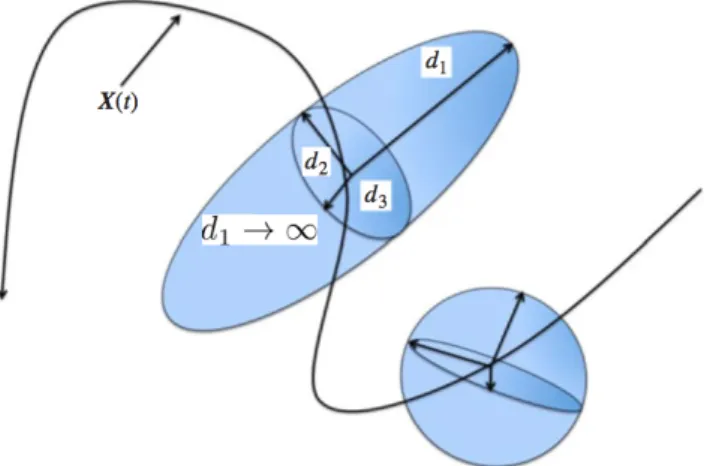
Generally speaking, the equation of motion for a rod-like particle (ellipsoid in the limit of infinity aspect-ratio see Fig.
1) in a turbulent velocity field u(r, t) is considered. The rod is assumed to be naturally buoyant and smaller than the smallest length scale characterizing fluid motion, i.e. the Kolmogorov length lη, but sufficiently large that their
Brow-nian motion do not need be considered. The motion of the rod or "tumbling rate" is determined by the particle orienta-tion and the velocity gradient tensor (as a particular case of the general Jeffery’s equation (Jeffery 1922)):
˙
pi= Ωijpj+ Sijpj− pipkSklpl (1)
where p is a unit director along the symmetric axis of the par-ticle, and SijandΩijare the symmetric and skew-symmetric
parts of the velocity gradient tensor, respectively. However,
Figure 1: (Colour online) Typical ellipsoidal shape of a fluid element along the turbulent trajectory. The fluid element center of mass X(t) is supposed to follow the evolution of the fluid particle and the deformation is governed by the statistics of the fluid velocity gradients along the trajectory, ∂iuj(X(t), t). The fluid element is always assumed of
el-lipsoidal shape with the three semi-axes ordered as d1⩾ d2⩾
d3. The rod-like particle is described by taking d1→ ∞. This
figure is adapted fromBiferale et al.(2014).
this approach leads to a non-linear equation that in the frame-work of stochastic modeling is difficult to deal with. The same dynamics can be solved by considering a linear equa-tion for the separaequa-tion of two fluid particles, particularly, the equation of motion has been derived considering the dynam-ics of two fluid tracers described by the vector R12and
even-tually normalizing the solution.
In more detail, the separation vector R12 = R1− R2
be-tween two fluid particles with trajectories Rn(t) = R(t; rn)
passing at t= 0 through the points rnsatisfies the equation
˙
R12(t) = v(R1, t) − v(R2, t). (2)
In the rest of the paper the subscript R12 is replaced by R.
Considering an incompressible fluid flow where the particles generally separate. In smooth velocity field, for separation R much smaller than the viscous scale of turbulence l≪ lη, i.e.
the so-called Batchelor regime (Batchelor 1959), the veloc-ity difference between two fluid particles can be expressed as v(R1, t) − v(R2, t) ≈ Aij(t)R with the Lagrangian strain
matrix Aij = ∂ui/∂xj(R2(t), t). In this regime, Eq. (2)
sim-plifies to the ordinary differential equation ˙
R(t) = Aij(t)R(t) (3)
leading to the linear solution
R(t) = Wij(t)R(0) (4)
where Wij is evolution matrix or the deformation gradient
tensor that characterizes the distortion withstand to the fluid element. The evolution matrix provides a Lagrangian de-scription of the fluid stretching. In other words, for three-dimensional flows, this process can be visualized by consid-ering a sphere that is distorted into a tri-axial ellipsoid ad it is stretched by the flow (see Fig.1). This means that pas-sive vectors along with thin rods-like become preferentially
aligned with the longest principal axis of the ellipsoid, and at long times approach (after10τη) perfect alignment with
the eigenvector corresponding to the maximum stretching has been studied byNi et al.(2014).
The general solution for the three dimensional case is de-termined by products of random matrices. The evolution ma-trix Wijmay be written as
Wij(t) = T exp [ ∫ t 0 Aij(s)ds] =∑∞ n=0∫ t 0 Aij(sn)dsn⋯ ∫ s3 0 Aij(s3)ds2∫ s2 0 Aij(s2)ds1 (5) This time-order exponential form (T ), in general, is not very useful for the direct computation except the particular case of a short correlated strain (see sec.Stochastic model for the orientation). The basic idea of the present approach, relies on the result that, in almost realization of the strain gradi-ent tensor, the matrix1/t ln WijWjistabilizes as t→ ∞ (see
Falkovich et al.(2001) for details). To give some intuitive in-sight, as already mentioned, considering some fluid volume, like a sphere, which evolves into an elongated ellipsoid at later time. As time increases, the ellipsoid is more and more elongated; furthermore the long time evolution of Eq. (3) is characterized by the following result
λL= lim t→∞ 1 tln( ∣ R(t)∣ ∣R(0)∣) (6) which for large t tends with probability one to the largest Lyapunov exponent λL (finite value), governing the chaotic
properties of the particles trajectories in the turbulent flow. In this way it is possible to solve the rod-like orientation through a linear ordinary differential equation Eq. (3); where the initial conditions are Wij(0) = I (identity matrix) and
R(0) = p(0). The solution for rod orientation in Eq. (1) is obtained by normalizing the solution of Eq. (3):
p(t) = R(t)
∣∣R(t)∣∣. (7)
Stochastic model for the orientation
The evolution of p depends upon the velocity gradient ten-sor Aij(t), therefore a stochastic model for it is presented.
Other Lagrangian stochastic model are present in literature, but so far this description has been always investigated in the framework of direct numerical simulations (DNS). Gaussian processes have been proposed for the velocity gradient statis-tics. For instance,Pumir and Wilkinson(2011) andVincenzi
(2013) have considered an Ornstein-Uhlenbeck process for Aij with a different correlation time scale for the
symmet-ric and skew-symmetsymmet-ric parts. This is more realistic, since it is known that in turbulence the correlation time scale for the rotation rate is significantly longer than that the strain rate. Otherwise, more refined model for the velocity gradient has been obtained byChevillard and Meneveau(2006), intro-ducing the RFDA model, which overcomes the Gaussian de-scription, predicting a variety of local, statistical, geometric
and anomalous scaling properties of 3-D turbulence. It is im-portant to mention as a reference, the work ofChevillard and Meneveau(2013); which examines in very detail the orienta-tion dynamics of the anisotropic particle in isotropic homo-geneous turbulence, using both DNS and different stochas-tic models. In this framework it is important to underline that these models are tested in a DNS context, or rather, they have been developed for an observation time of the order of the Kolmogorov timescale (τ≃ τη).
The solution of the differential equation such as Eq. (3) with a stochastic input Aijis given by Eq. (5) with the matrix
Wij(t) involving stochastic integrands over the time. The
case of a short correlated velocity gradient tensor ( Kraich-nan 1968) allows for a complete solution. More specifically, when the observation time of the dynamics is much larger than the correlation time of the velocity gradient tensor, i.e. t≫ τη, Wijmay be viewed as a continuous product of
inde-pendent random matrix. Under this assumption, the instan-taneous velocity gradient tensor can be decomposed in two contributions: mean field and fluctuations
Aij(X(t, ω), t) = ⟨∂iuj(X(t, ω), t)⟩ + ξij(t, ω) (8)
where the⟨⋅⟩ means the ensemble average and ξij(t, ω) is a
white-noise that can be rewritten as dFij(t, ω) = ξij(t, ω)dt.
This stochastic forcing (fluctuation) is of the form dFij =
bijkldWkl, where dWkl represent a Wiener process, i.e
⟨Wij⟩ = 0 and ⟨dWijdWkl⟩ = δikδjldt leading to,
⟨dFijdFkl⟩ = bijmnbmnkldt (9)
Incompressibility, isotropy and parity invariance impose the form of the fourth-order tensor bijkl,
bijkl= b1δijδkl+ b2δikδjl+ b3δilδjk. (10)
with the coefficients b1 = (−
√ 3/3)/τ2 η, b2 = 0.5( √ 3 + √ 5)/τ2 η and b3 = 0.5( √ 3−√5)/τ2
η which depend
exclu-sively on the Kolmogorov time scale τη (see Johnson and
Meneveau(2016) for details).
Now, replacing the decomposition for Aij into the rods’
orientation Eq. (3), it is possible to re-formulate the stochas-tic differential equation (SDE)
dRi(t) = ⟨Aij⟩ Rjdt+ dFij○ Rj (11)
interpreted in the Stratonovich form (○). The natural form for a direct calculation of the SDE is the Itô form, so applying the transformation from Stratonovich to Itô the SDE in the index notation becomes
dRi=(¯aii+ 1 2((b1+ b2+ b3) 2+ 2b2 1))Ridt +∑3 j=1 ¯ aijRj(1 − δij)dt + ((b2+ b3)dWii+ b1 3 ∑ j=1 dWjj)Ri + (b2+ b3) 3 ∑ j=1 Rj(1 − δij)dWij (12)
where¯aij are the elements of ⟨Aij⟩ and dWij is a matrix
composed by nine independent Brownian motion. Here, the repeated index is not an implicit summation and δij is the
Kronecker’s symbol. To attain the complete description of the rod’s orientation p the SDE is coupled with the normal-ization procedure, as outlined in the Eq. (7).
It is worth to notice that, when the observation time-step ∆t becomes smaller with respect to the Kolmogorov inner time scale τηthe model for the orientation is no longer valid.
This constraint reflects the argument that on a large enough observation time scale (meaning precisely ∆t ≫ τη), the
stochastic model for the orientation is coherent with the phys-ical description of the Lagrangian stochastic model. In par-ticular, it should be stressed that there is a strong interplay between the physical aspects of the model (which leads to a formulation in terms of SDE) and the numerical aspects of the practical simulations as also has been remarked byMinier et al.(2001).
Results and Discussion
This section presents some results obtained from the nu-merical simulations of the Lagrangian stochastic model de-scribed by Eq. (12) and Eq. (7). The model has been performed using a numerical integration scheme based on splitting algorithm, which solves the symmetric and skew-symmetric part of the velocity gradient tensor separately (Campana et al. N.D.). The validation has been restricted to the homogeneous isotropic turbulent (HIT) case, so that the mean velocity gradient tensor is assumed to be zero ( ⟨Aij⟩ = 0). As discussed above, the validation of the
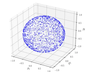
model has to be performed for an integration time-step big-ger than the Kolmogorov one. Three simulations have been performed: varying the value of the ratio between the obser-vation timescale and the Kolmogorov time scale (the setup for three different cases are detailed in Tab. 1). Indepen-dent sample of rods have been initialized at time zero, im-posing to each of them a uniform distribution on the unit sphere (U(S2)) for the three cases. In the context of HIT, due to the hypotheses of homogeneity and isotropy of the fluid field, the rod orientation vector should remain uniformly dis-tributed on the unit sphere. Firstly, results are presented in the Cartesian coordinate system. The whole sample of orien-tation vectors p remain, for long time simulation, distributed on the unit sphere as showed in Fig.2. Regarding the first and second moments of the orientation vector (p1, p2, p3),
the Tab.2presents measures of the error of mean and vari-ance of the stochastic process evaluating at final time. The empirical mean of any generic moments is denoted as
⟨f(p)⟩M C =
1 Npsample∑
f(psimualtions) (13)
and the error is usually decomposed in two contributions: the bias part due to the integration scheme and the Monte Carlo error due to the size of sample as,
E(E[f(p)] − ⟨f(p)⟩M C) 2 = O(∆t2α) + O(Var(f(p)) Np ) (14) p1 −1.0 −0.5 0.0 0.5 1.0 p2 −1.0 −0.5 0.0 0.5 1.0 p3 −1.0 −0.5 0.0 0.5 1.0
Figure 2: (Colour online) Sample orientation vector evalu-ated at finale time (T = 103) distributed on the sphere with a number of iterations105for the case 3.
Setup ∆t τ/τk Np T I.d
Case 1 0.01 1 105 103 U(S2)
Case 2 0.1 10 105 103 U(S2)
Case 3 1 100 105 103 U(S2)
Table 1: Summary of the simulations performed for the La-grangian stochastic model. For each cases the parameters are referred to: the time-step (∆), the ratio between the observa-tion and Kolmogorov timescales (τ/τk), the numbers of
par-ticles used to performed the Monte Carlo (MC) simulations (Np), the final time (T ) and the initial distribution imposed
(I.d).
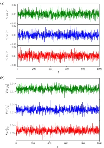
The values of the errors are listed in Tab.2; these are small and of the same order for the three values of the integration time-step∆t. The explanation of this last result relies into the fact that, analyzing the two sources of error, it appears that the total error is dominated by the Monte Carlo approx-imation, even for the large integration time-step. In Fig.3is presented the time evolution of the mean and variance of the rod orientation vector. Both of the mean (see Fig.3a) and variance (see Fig.3b) account for the ergodicity of the simu-lated process. This fact is of main importance regarding the construction of the model (Eq.6), as discussed above. In fact, the mean oscillates around zero (which is the exact value) for the three component of the orientation vector p (see Fig.3a) with an error (Tab.2) that is produced only by the MC sim-ulations for the three cases. Similar remarks can be done looking the variance (see Fig.3b), in this case the value of the components of p fluctuating around the exact value of 1/3 for each of them (Tab.2).
To complete the description of the numerical results and to have, at the same time, a more physical characterization of the model itself, the results on the empirical probability distribution function (p.d.f ) are presented. To analyze the
(a) −0.02 0.00 0.02 < p1 > −0.02 0.00 0.02 < p2 > 0 200 400 600 800 1000 t −0.02 0.00 0.02 < p3 > (b) 0.33 0.34 V ar[ p1 ] 0.33 0.34 V ar[ p2 ] 0 200 400 600 800 1000 t 0.33 0.34 V ar[ p3 ]
Figure 3: (Colour online) Mean (a) and variance (b) for the three component of the orientation vector p as a function of time, obtained for the case 3.
Error Case 1 Case 2 Case 3
∣E[pi] − ⟨pi⟩M C∣ 0.00157 0.00360 0.00089 0.00113 0.00005 0.00046 0.00028 0.00019 0.00172 ∣E[p2 i] − ⟨p2i⟩M C∣ 0.00060 0.00019 0.00092 0.00079 0.00021 0.00117 0.00138 0.00005 0.00211 ∣E[g] − ⟨g⟩M C∣ 0.00005 0.00023 0.00023
Table 2: Estimation of the weak error for the first, second moment and the function g = g(p1, p2, p3) = p1p2p3. The
piindicates the exact value, the computed one. The table is
organized as following: the error for the mean and variance is computed for each coordinates in order i= 1, 2, 3.
orientation dynamics on a non-spherical particle, it is con-venient to move from Cartesian coordinates (p1, p2, p3) to
spherical coordinates(r, ϕ, θ) according to the usual trans-formations r=√p2 1+ p22+ p23, ϕ= arctan (√p2 1+ p 2 2/p3), θ= arctan(p2/p1) (15)
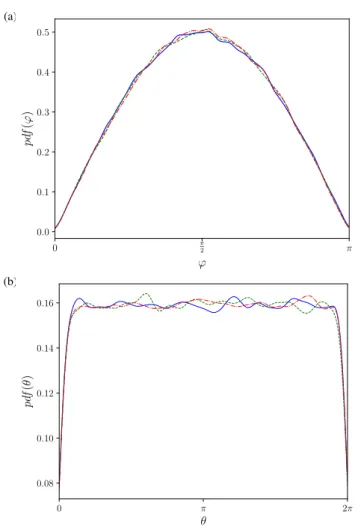
with r ⩾ 0, 0 ⩽ ϕ ⩽ π and 0 ⩽ θ ⩽ 2π. In Fig.4 are pre-sented the marginal distributions for the two spherical an-gles: the Fig.4aand Fig.4b) show respectively the empiri-cal pdf(ϕ) and pdf(θ) for the three cases. The three corre-sponding curves are all in good agreement with the theoreti-cal marginals p.d.f : p.d.f(θ)th= 1 4π ∫ π 0 sin ϕdϕ= 1 2π p.d.f(ϕ)th= 1 4π ∫ 2π 0 sin ϕdθ= 1 2sin ϕ. (16)
Finally, on account of the unitary length of the orientation vector ∣∣p∣∣ (r = 1), the empirical joint probability density function of the orientation must take the form of p.d.f(ϕ, θ) in spherical coordinates. It is showed in Fig.5and its two-dimensional projection Fig. 6. This empirical p.d.f(ϕ, θ) has been obtained through the use a Gaussian smoothing ker-nel that wrings the surface near the boundaries of the plots. It appears that the empirical joint p.d.f is in agreement with the theoretical one,
p.d.f(ϕ, θ)th=
1
4πsin ϕ. (17)
Conclusions
In this study, the rod orientation is described by a La-grangian stochastic model using dedicated splitting scheme for time integration along large observation time-scale. The cumulative effects of the velocity gradient tensor are assumed fluctuating with a Gaussian distribution with short-time cor-relations. A new stochastic differential equation (SDE), which describes the separation between two fluid particles, has been proposed. This SDE coupled with a renormaliza-tion procedure provides the descriprenormaliza-tion of the rod’s orienta-tion. The model have been tested numerically in the HIT case and three reference time-scale orders have been exam-ined, showing a good agreement between theoretical and em-pirical, both for the marginal and joint probability density function expressed in spherical coordinates. This preliminary study serves as a base to go further both on the modeling and the numerical development.
Acknowledgments
This work has been supported by EDF R&D (projects PTHL of MFEE and VERONA of LNHE) and by the French government, through the Investments for the Future project UCA JEDI ANR-15-IDEX-01 managed by the Agence Na-tionale de la Recherche
(a) 0 π2 π ϕ 0.0 0.1 0.2 0.3 0.4 0.5 pd f (ϕ ) (b) 0 π 2π θ 0.08 0.10 0.12 0.14 0.16 pd f (θ )
Figure 4: (Colour online) P.d.f of the angle ϕ in (a) and θ in (b) in the spherical coordinates system. Results from case 1 (blue solid line), case 2 (green dashed line) and case 3 (red dot-dashed line). θ 0 π 2π ϕ 0 π 2 π 0.02 0.04 0.06 0.08 0.10 0.02 0.04 0.06 0.08 0.10 pdf (ϕ, θ)
Figure 5: (Colour Online) Empirical joint P.d.f in spherical coordinates produces with the case 3.
0 π 2π θ 0 π 2 π ϕ 0.02 0.04 0.06 0.08 0.10 pd f (ϕ, θ)
Figure 6: (Colour online) Projected empirical joint P.d.f in spherical coordinates produces with the case 3.
References
George K Batchelor. Small-scale variation of convected quantities like temperature in turbulent fluid part 1. general discussion and the case of small conductivity. Journal of Fluid Mechanics, 5(1):113–133, 1959.
Luca Biferale, Charles Meneveau, and Roberto Verzicco. De-formation statistics of sub-kolmogorov-scale ellipsoidal neu-trally buoyant drops in isotropic turbulence. Journal of fluid mechanics, 754:184–207, 2014.
Brett K Brunk, Donald L Koch, and Leonard W Lion. Ob-servations of coagulation in isotropic turbulence. Journal of fluid mechanics, 371:81–107, 1998.
Lorenzo Campana, Mireille Bossy, Minier Jean Pierre, and Christophe Henry. Numerical scheme for a lagrangian stochastic model describing rods orientation. unpublished, N.D.
Laurent Chevillard and Charles Meneveau. Lagrangian dynamics and statistical geometric structure of turbulence. Physical review letters, 97(17):174501, 2006.
Laurent Chevillard and Charles Meneveau. Orientation dy-namics of small, triaxial–ellipsoidal particles in isotropic tur-bulence. Journal of Fluid Mechanics, 737:571–596, 2013. G Falkovich, K Gawedzki, and M Vergassola. Particles and fields in fluid turbulence. Reviews of modern Physics, 73(4): 913, 2001.
Andrew J Heymsfield. Precipitation development in strati-form ice clouds: A microphysical and dynamical study. Jour-nal of the Atmospheric Sciences, 34(2):367–381, 1977. George Barker Jeffery. The motion of ellipsoidal particles immersed in a viscous fluid. Proc. R. Soc. Lond. A, 102(715): 161–179, 1922.
Perry L Johnson and Charles Meneveau. A closure for lagrangian velocity gradient evolution in turbulence us-ing recent-deformation mappus-ing of initially gaussian fields. Journal of Fluid Mechanics, 804:387–419, 2016.
RH Kraichnan. Rh kraichnan, phys. fluids 11, 945 (1968). Phys. Fluids, 11:945, 1968.
Fredrik Lundell, L Daniel Söderberg, and P Henrik Alfreds-son. Fluid mechanics of papermaking. Annual Review of Fluid Mechanics, 43:195–217, 2011.
Charles Meneveau. Lagrangian dynamics and models of the velocity gradient tensor in turbulent flows. Annual Review of Fluid Mechanics, 43:219–245, 2011.
Jean-Pierre Minier et al. Probabilistic approach to turbulent two-phase flows modelling and simulation: theoretical and numerical issues. Monte Carlo Methods and Applications, 7 (3/4):295–310, 2001.
Ryan C Moffet and Kimberly A Prather. In-situ measure-ments of the mixing state and optical properties of soot with implications for radiative forcing estimates. Proceedings of the National Academy of Sciences, 106(29):11872–11877, 2009.
PH Mortensen, HI Andersson, JJJ Gillissen, and BJ Boersma. Dynamics of prolate ellipsoidal particles in a turbulent chan-nel flow. Physics of Fluids, 20(9):093302, 2008.
Magdalena M Musielak, Lee Karp-Boss, Peter A Jumars, and Lisa J Fauci. Nutrient transport and acquisition by diatom chains in a moving fluid. Journal of Fluid Mechanics, 638: 401–421, 2009.
Rui Ni, Nicholas T Ouellette, and Greg A Voth. Alignment of vorticity and rods with lagrangian fluid stretching in tur-bulence. Journal of Fluid Mechanics, 743, 2014.
Alain Pumir and Michael Wilkinson. Orientation statistics of small particles in turbulence. New journal of physics, 13(9): 093030, 2011.
Lilach Sabban and René van Hout. Measurements of pollen grain dispersal in still air and stationary, near homogeneous, isotropic turbulence. Journal of Aerosol Science, 42(12): 867–882, 2011.
Mansoo Shin and Donald L Koch. Rotational and transla-tional dispersion of fibres in isotropic turbulent flows. Jour-nal of Fluid Mechanics, 540:143–173, 2005.
Dario Vincenzi. Orientation of non-spherical particles in an axisymmetric random flow. Journal of Fluid Mechanics, 719: 465–487, 2013.
Michael Wilkinson and HR Kennard. A model for alignment between microscopic rods and vorticity. Journal of Physics A: Mathematical and Theoretical, 45(45):455502, 2012. Haifeng Zhang, Goodarz Ahmadi, Fa-Gung Fan, and John B McLaughlin. Ellipsoidal particles transport and deposition in turbulent channel flows. International Journal of Multiphase Flow, 27(6):971–1009, 2001.