Deformation of a flexible polymer in a random flow with long correlation time

(1)

HAL Id: hal-00544362

https://hal.archives-ouvertes.fr/hal-00544362

Submitted on 8 Dec 2010

HAL is a multi-disciplinary open access

archive for the deposit and dissemination of

sci-entific research documents, whether they are

pub-lished or not. The documents may come from

teaching and research institutions in France or

abroad, or from public or private research centers.

L’archive ouverte pluridisciplinaire HAL, est

destinée au dépôt et à la diffusion de documents

scientifiques de niveau recherche, publiés ou non,

émanant des établissements d’enseignement et de

recherche français ou étrangers, des laboratoires

publics ou privés.

Deformation of a flexible polymer in a random flow with

long correlation time

Stefano Musacchio, Dario Vincenzi

To cite this version:

Stefano Musacchio, Dario Vincenzi. Deformation of a flexible polymer in a random flow with long

correlation time. Journal of Fluid Mechanics, Cambridge University Press (CUP), 2011, 670,

pp.326-336. �10.1017/S0022112010006385�. �hal-00544362�

(2)

J. Fluid Mech., in press 1

Deformation of a flexible polymer in a

random flow with long correlation time

S T E F A N O M U S A C C H I O

A N D

D A R I O V I N C E N Z I

CNRS UMR 6621, Laboratoire J.A. Dieudonn´e, Universit´e de Nice Sophia Antipolis, Parc Valrose, 06108 Nice, France

The effects induced by long temporal correlations of the velocity gradients on the dynam-ics of a flexible polymer are investigated by means of theoretical and numerical analysis of the Hookean and FENE dumbbell models in a random renewing flow. For Hookean dumbbells, we show that long temporal correlations strongly suppress the Weissenberg-number dependence of the power-law tail characterising the probability density function (PDF) of the elongation. For the FENE model, the PDF becomes bimodal, and the coil–stretch transition occurs through the simultaneous drop and rise of the two peaks associated with the coiled and stretched configurations, respectively.

1. Introduction

The dynamics of a flexible polymer in a moving fluid depends strongly on the properties of the velocity gradients. A remarkable example is given by the coil–stretch transition in a planar extensional flow v = (²x, −²y) (de Gennes 1974; Perkins, Smith & Chu 1997). This flow is characterised by a direction of pure compression and a direction of pure stretching with constant strain rate ². The elongation of the polymer is controlled by the Weissenberg number Wi = ²τp, where τp is the longest relaxation time of the polymer.

The value Wi = 1/2 marks the coil–stretch transition: for Wi < 1/2 the polymer remains coiled under the action of the entropic elastic force, whereas for Wi > 1/2 the drag force exerted by the flow overcomes the entropic force and the polymer unravels almost completely. As a consequence, the probability density of the extension, p(R), has a single pronounced peak, whose position depends on Wi. For Wi < 1/2, the peak is in the neighbourhood of the equilibrium size of the polymer, R0; for Wi > 1/2, the peak

approaches the maximum length Rmax.

The ability of a (non-uniform) laminar flow to deform an isolated polymer has now been demonstrated for various flow configurations (see, e.g., the reviews by Larson 2005 and Shaqfeh 2005). The corresponding problem for random flows was first studied by Lumley (1972, 1973), who observed that the strain tensor of an incompressible random flow always has a direction of stretching, although such direction fluctuates in time and in space. Lumley further remarked that the vorticity penalises polymer stretching, for it pre-vents the polymer from remaining aligned with the principal axes of the strain tensor. He then concluded that random flows can stretch polymers if the product of the Lagrangian correlation time of the strain tensor and the modulus of the maximum eigenvalue of the deformation tensor exceeds a critical value proportional to τ−1

p . Groisman &

Stein-berg (2001) confirmed these conclusions by showing evidences of a significant amount of polymer stretching in a low-Reynolds-number random flow generated by viscoelastic instabilities.

In random flows, the time scale describing the stretching of line elements is the re-ciprocal of the maximum Lyapunov exponent λ. Hence the appropriate definition of the Weissenberg number is Wi = λτp. Balkovsky, Fouxon & Lebedev (2000) and Chertkov

(3)

(2000) related the deformation of a polymer in a random flow to the statistics of the stretching rate or, more precisely, to the entropy function associated with its probabil-ity densprobabil-ity function (e.g., Crisanti, Paladin & Vulpiani 1993). Based on this analysis, Balkovsky et al. (2000) predicted the existence of the coil–stretch transition for any random flow with positive λ, and proposed the following explanation. For an infinitely extensible polymer (Rmax → ∞), the stationary probability density function (PDF) of

the extension has a power-law tail: p(R) ∝ R−1−α _{for R À R}

0, where α depends on

the form of the entropy function. The exponent α is positive for Wi < 1/2, it decreases with increasing Wi, and becomes negative as Wi exceeds 1/2. Consequently, p(R) is normalizable only for Wi < 1/2, whereas for Wi > 1/2 there is unbounded growth of the extension and the assumption of infinite extensibility becomes inadequate. This abrupt change in the statistics of the extension is interpreted as indicating the coil–stretch tran-sition in random flows. The threshold Wi = 1/2 reproduces (to within a numerical factor) Lumley’s criterion†.

If the random flow is isotropic and has zero correlation time, p(R) can be written explicitly and the behaviour predicted by Balkovsky et al. (2000) can be obtained by direct computation (Chertkov 2000; Thiffeault 2003; Celani, Musacchio & Vincenzi 2005; Martins Afonso & Vincenzi 2005). In this particular case, α = d(Wi−1− 2)/2, where d

is the spatial dimension of the flow.

A polymer having finite maximum extension (Rmax< ∞) reaches a stationary

configu-ration at any Wi since the entropic force forbids extensions greater than Rmax. According

to the analysis of the infinitely extensible case, p(R) is now expected to display a power-law behaviour R−1−α _{for R}

0 ¿ R ¿ Rmax. In a short-correlated flow, the coil–stretch

transition results from the combination of this power law and the cutoff at R = Rmax:

as Wi increases, the intermediate power law raises and the peak of p(R) moves from R0

to extensions near to Rmax(Martins Afonso & Vincenzi 2005). An important qualitative

difference between extensional and random flows must nevertheless be emphasised. In the former case, p(R) has a pronounced peak at an extension near either R0 or Rmax

depending on whether Wi is less or greater than 1/2. In the latter case, p(R) has broad tails signaling the coexistence of coiled and stretched configurations with predominance of either configuration according to the value of Wi. In random flows, the coil–stretch transition is not as sharp as in the extensional case because of the random nature of the velocity gradient and the presence of vorticity.

The coil–stretch transition and the relation between the exponent α and the maximum Lyapunov exponent λ were investigated experimentally by Gerashchenko, Chevallard & Steinberg (2005) and Liu & Steinberg (2010). In these experiments, the statistics of the extension was measured by following a fluorescently labelled polymer in a random velocity field generated by elastic turbulence. The PDF of polymer extension was also investigated by means of direct numerical simulations of the continuum equation for the polymer conformation tensor (Eckhardt, Kronj¨ager & Schumacher 2002; Boffetta, Celani & Musacchio 2003) and by means of Brownian Dynamics simulations for elastic dumbbells (Celani et al. 2005; Davoudi & Schumacher 2006; Bagheri et al. 2010) or multi-bead chains (Watanabe & Gotoh 2010). The results of the simulations support the picture of polymer dynamics presented above.

The Weissenberg number suffices to determine the elongation of a polymer in laminar flows. By contrast, in random flows an additional dimensionless number may influence the deformation of the polymer, namely, the Kubo number Ku = λτc, where τc is the

† Balkovsky et al. (2000) defined the Weissenberg number as Wi = 2λτp so that the

(4)

Deformation of a polymer in a random flow with long correlation time 3 Lagrangian correlation time of the velocity gradient. The case Ku = 0 has been briefly reviewed above. In this paper, we examine the effect of a nonzero Ku and show that the dynamics at Ku > 1 differs significantly from the one predicted for short-correlated flows. To emphasise the basic physical mechanisms, we consider a simplified situation. The poly-mer molecule is modelled as an elastic dumbbell (Bird et al. 1977). This approximation is appropriate when attention is restricted to the extension of the polymer (Watanabe & Gotoh 2010). As for the random advection, we consider a two-dimensional linear renew-ing flow. In renewrenew-ing flows, time is split into intervals of length τc and the velocities in

different intervals are independent and identically distributed (e.g., Childress & Gilbert 1995, p. 320). Linear renewing flows were used by Zel’dovich et al. (1984) to study the kinematic dynamo effect. The magnetic field is actually stretched by the velocity gradient in the same way as an infinitely extensible polymer. The use of a linear renewing flow enables us to obtain semi-analytical results and to accurately compute the statistics of polymer extension with moderate numerical effort.

The remainder of the paper is divided as follows. In section 2, we briefly review the elastic dumbbell model. In section 3, we introduce the renewing random flow. The results are presented in section 4. Finally, some conclusions are drawn in section 5.

2. Elastic dumbbell model

An elastic dumbbell is composed of two beads joined by a spring. The beads repre-sent the two ends of the polymer; the spring models the entropic force. For the sake of simplicity, we assume that the flow transporting the dumbbell is two-dimensional.

The vector separating the ends of the polymer, R, satisfies the stochastic ordinary differential equation (e.g., Bird et al. 1977):

˙ R = σ(t)R − 1 2τp f (R)R + s R2 0 τp ξ(t), (2.1)

where R = |R| and ξ(t) is white noise, i.e., a Gaussian process with zero mean and two-time correlation hξi(t)ξj(t0)i = δijδ(t − t0). The three terms on the right-hand-side

of equation (2.1) result from the drag force, the entropic elastic force, and thermal noise, respectively. The 2×2 matrix σ(t) is the velocity gradient evaluated along the trajectory of the centre of mass of the dumbbell: σij(t) = ∂jvi(t). The function f (R) is identically equal

to 1 for an infinitely extensible polymer (Hookean model) and has the form f (R) = 1/(1−

R2_/R2

max) for a finitely extensible polymer with nonlinear elasticity (FENE model). In

the former case, R is defined on R2_{; in the latter case, R belongs to [0, R}

max) × [0, Rmax).

Equation (2.1) holds under some assumptions on the dynamics of the beads. The velocity field is assumed to be linear at the size of the dumbbell. The drag on a bead is given by the Stokes law. Furthermore, hydrodynamic interactions between the beads and inertial effects are disregarded.

3. Linear renewing flow

According to the assumptions of the dumbbell model, in the reference frame of the centre of mass of the polymer the velocity field is of the form: vi(r, t) = σij(t)rj. The

velocity gradient σ(t) is constant in each of the time intervals In= [nτc, (n+1)τc), n ∈ N.

We denote by σn the (random) value taken by σ(t) in In: σ(t) = σn for all t ∈ In. The

random matrices σnare identically distributed and statistically independent. We assume

(5)

that the velocity field is incompressible). As a result, σ(t) takes the form: σ(t) = S 2 µ ζ1(t) ζ2(t) ζ2(t) −ζ1(t) ¶ +√Ω 2 µ 0 ζ3(t) −ζ3(t) 0 ¶ (3.1) with S and Ω positive constants. The elements ζi(t) satisfy: ζi(t) = ζi,n for all t ∈ In,

where the ζi,n are Gaussian random variables such that hζi,ni = 0 for all i and n and

hζi,nζj,mi = δijδnm for all i, j = 1, 2, 3 and n, m ∈ N. The mean-squared strain and

rotation rates are S2 _{and Ω}2_{, respectively. We set Ω = S to reproduce the relation}

holding for the solution of the Navier–Stokes equation (e.g., Frisch 1995, p. 20).

Strictly speaking, the flow considered is not statistically stationary in time. Neverthe-less, over time ranges longer than τc, it can be considered as a good approximation to

a stationary flow with correlation time τc owing to the invariance with respect to the

transformation t → t+τcand thanks to the independence of the matrices σ(t) in different

time intervals In (Zel’dovich et al. 1984). The δ-correlated flow (i.e. white-in-time noise)

is recovered by letting τc tend to zero while holding S2τc constant.

As mentioned in the introduction, the elongation of a polymer is related to the statistics of the stretching rate of the flow. For a review on the entropy function and the generalized Lyapunov exponents in statistical physics, we refer the reader to the book by Crisanti et al. (1993). Here, we briefly recall some basic elements of the theory. If `(t) denotes a fluid-line element, the stretching rate at time t is defined as γ(t) = t−1_{ln[`(t)/`(0)].}

The maximum Lyapunov exponent is the long-time limit of the average stretching rate:

λ = limt→∞hγ(t)i, where the average is taken over the realizations of σ(t). The PDF of γ

for long t takes the large-deviation form (Crisanti et al. 1993):

P (γ, t) ∝ e−G(γ)t,

where G(γ) is the entropy function. G(γ) is non-negative and attains its minimum value at the point λ. Equivalently, the stretching properties of the flow can be characterised by the generalized Lyapunov exponents, defined as the rate of growth of the moments of `(t): L(q) = lim t→∞ 1 t ln ¿µ `(t) `(0) ¶qÀ .

The function L(q) is the Legendre transform of G(γ), L(q) = maxγ[γq − G(γ)], and

sat-isfies L0_{(0) = λ. For small q, L(q) can be obtained by using the quadratic approximation}

G(γ) ≈ (γ − λ)2_{/(2∆) so that L(q) ≈ λq + ∆q}2_/2.

For the linear renewing flow, we can compute L(q) by adapting to the present problem the method described by Gilbert & Bayly (1992) (see also Childress & Gilbert 1995, pp. 322–326). A line element satisfies the equation:

˙`(t) = σ(t)`(t). (3.2)

Since σ(t) is constant in In, the solution of equation (3.2) for t ∈ In is: `(t) = eσnt`(nτc).

Hence `((n + 1)τc) = Jn`(nτc), where Jn= eσnτc is written Jn= 1 2ωn   2ωnc+n + Sζ1,nc−n (Sζ2,n+ √ 2Ωζ3,n)c−n (Sζ2,n− √ 2Ωζ3,n)c−n 2ωnc+n − Sζ1,nc−n   with ωn = 1₂ q S2_(ζ2 1,n+ ζ2,n2 ) − 2Ω2ζ3,n2 , c+n = (eωnτc + e−ωnτc)/2, and c−n = (eωnτc−

(6)

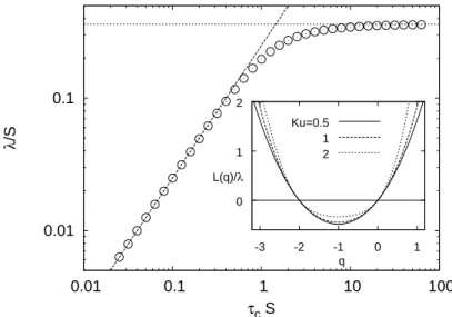
Deformation of a polymer in a random flow with long correlation time 5 0.01 0.1 0.01 0.1 1 10 100 λ /S τc S 0 1 2 1 0 -1 -2 -3 q L(q)/λ Ku=0.5 1 2

Figure 1. Lyapunov exponent as a function of τc(circles). Dashed and dotted lines represent the

asymptotic behaviours (3.5) for τc→ 0 and τc→ ∞, respectively. Inset: Generalized Lyapunov

exponents L(q) for three values of Ku. Note that L(−d) = L(0) = 0 in agreement with the properties of the generalized Lyapunov exponents proved by Zel’dovich et al. (1984).

e−ωnτc_{)/2 (we remind the reader that ζ}

i,n is the constant value taken by the random

function ζi(t) in In). If ωnis real, then Jncan be written in terms of hyperbolic functions;

for a non-real complex ωn, Jn involves trigonometric functions. By using the statistical

isotropy of the flow and the fact that the matrices σn are identically distributed and

independent for different n, it is possible to show the following relation (Gilbert & Bayly 1992; Childress & Gilbert 1995):

h`q_{((n + 1)τ} c)i

h`q_(nτ_c_)i = h|Jne| q_i

In, (3.3)

where e is any constant unit vector and the average h·iIn is taken over the statistics of the gradient in the interval Inonly. Iterating equation (3.3) yields: h`q(nτ )i = hρqinIn`

q₍₀₎

with ρ2_{≡ |J}

ne|2= eTJnTJne. It follows that L(q) and λ can be written as

L(q) = τ−1

c lnhρqiIn and λ = τ

−1

c hln ρiIn. (3.4) Given that the σn are identically distributed, the average can be taken over any

in-terval In. Equations (3.4) provide a simple way to compute the function L(q) and the

Lyapunov exponent. The behaviour of λ as a function of τc is reported in figure 1. The

following asymptotic behaviours hold (Chertkov et al. 1996):

λ ∼ S 2_τ c 4 (τc→ 0) and λ ∼ RehωniIn= r π 2 S 2 r S2 S2_{+ 2Ω}2 (τc→ ∞). (3.5) For Ω = S, one obtains λ ∼ pπ/6 S/2 as τc → ∞. Thus the Lyapunov exponent

becomes independent of τc for large τc, and the convergence to the asymptotic value is

exponential. By contrast, the variance ∆ monotonically increases like ∆ ∼ S2_τ

c/4 both

for small and large τc (Chertkov et al. 1996), and therefore the generalized Lyapunov

(7)

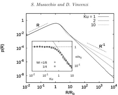
1 10-2 10-4 10-6 10-8 104 103 102 10 1 10-1 10-2 p(R) R/R₀ R R-1 Ku = 1 2 10 1 10-2 10-4 10-6 10-8 104 103 102 10 1 10-1 10-2 p(R) R/R₀ R R-1 1 10-2 10-4 10-6 10-8 104 103 102 10 1 10-1 10-2 p(R) R/R₀ R R-1 10 1 10-1 10-2 1 10-1 Ku α/α0 Wi =1/8 1/4

Figure 2. PDFs of polymer elongation, p(R), for the Hookean model at Wi = 1/4. Note the power-law behaviours p(R) ∝ Rd−1_{for R ¿ R0}_{and p(R) ∝ R}−1−α_{for R À R0. Inset: Exponent}

α as a function of Ku. Here α0= limKu→0α. Dash-dotted and dashed lines are the asymptotic

behaviours (4.1) and (4.2) for Ku → 0 and Ku → ∞, respectively.

asymptotic behaviours hold for any two-dimensional random flow that is incompressible and statistically isotropic and not only for the renewing flow.

4. Statistics of polymer extension

In order to investigate the influence of temporal correlations of the velocity gradients on the dynamics of polymers, we numerically integrated equation (2.1) for the elastic dumbbell model, where the velocity gradients were determined by equation (3.1). We computed the PDF of the polymer elongation R for various values of Ku and Wi. The numerical integration has been performed using the predictor–corrector scheme proposed by ¨Ottinger (1996) for the FENE model and the stochastic Runge–Kutta algorithm intro-duced by Honeycutt (1992) for the Hookean model. The statistics of polymer elongation has been computed by following the dynamics of a single dumbbell for 107 _time

inter-vals In.

Within the Hookean model, the PDF of the extension behaves like p(R) ∝ R−1−α _for

R À R0 (Balkovsky et al. 2000). The coil–stretch transition is identified by the change

of sign of α, which occurs at Wi = 1/2. The effects of the temporal correlation of the velocity gradients can be quantified through the dependence of α on the Kubo number. The numerical simulations of the Hookean model show that for small values of Ku the tail of p(R) is almost independent of Ku; conversely, for Ku & 1, the tail raises as Ku increases and approaches the slope −1 (figure 2). Because of long temporal correlations, even polymers with a short relaxation time occasionally experience significant stretching events, and this effect produces a power-law tail close to the coil–stretch transition also for small values of Wi.

This intuitive idea can be rationalized by the following argument. The exponent α determines the lowest order such that hRα_{i diverges and satisfies α = 2τ}

pL(α) (Boffetta

et al. 2003). For Wi near to 1/2, α is not far from zero and it is appropriate to use the quadratic approximation for L(q). The equation α = 2τpL(α) then yields (Balkovsky et

(8)

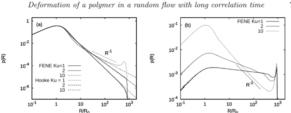
Deformation of a polymer in a random flow with long correlation time 7 1 10-2 10-4 10-6 103 102 10 1 10-1 p(R) R/R0 (a) R-1 FENE Ku=1 2 10 Hooke Ku = 1 2 10 1 10-2 10-4 10-6 103 102 10 1 10-1 p(R) R/R0 (a) R-1 10-1 10-2 10-3 10-4 103 102 10 1 10-1 p(R) R/R0 (b) R-1 FENE Ku=1 2 10 10-1 10-2 10-3 10-4 103 102 10 1 10-1 p(R) R/R0 (b) R-1

Figure 3. PDFs of polymer elongation, p(R) for the FENE model at various values of Ku for

Wi = 1/4 (panel (a)) and Wi = 1 (panel (b)). The maximum extension is set to Rmax= 103R0.

al. 2000): α = λ ∆ µ 1 Wi − 2 ¶ . (4.1)

While the dependence of α on the Weissenberg number is contained entirely in the second factor, the Kubo number enters the expression for α through the ratio λ/∆. For the linear renewing flow, the asymptotic behaviours discussed in section 3 give:

λ/∆ ∼ 1 (Ku → 0) and λ/∆ = O(Ku−1) (Ku → ∞). (4.2) One obtains that for small values of Ku the tail of p(R) is independent of Ku, whereas

α = O(Ku−1) as Ku is increased, in agreement with our numerical findings.

Although for an infinitely extensible polymer p(R) is normalizable only for α > 0 (equivalently for Wi > 1/2), the calculation leading to the power-law behaviour remains formally valid also if α < 0 (Wi > 1/2). In this case, the stationary PDF of the extension exists only if the nonlinearity of the elastic force is taken into account, and the power-law prediction is expected to hold for intermediate extensions R0¿ R ¿ Rmax. To allow the

development of the intermediate power law, we performed numerical simulations of the FENE model at artificially high Rmax/R0. For Wi < 1/2 the results agree with those

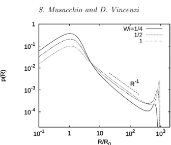
obtained for the Hookean model (figure 3, panel (a)). For Wi > 1/2 an increase of Ku produces a decrease of the intermediate slope of p(R), which can be negative even for very large Wi (figure 3, panel (b)). According to equation (4.2), near Wi = 1/2 the range of variation of α as a function of Wi can be made arbitrarily small by increasing Ku, to the extent that the intermediate slope of p(R) becomes almost independent of Wi (figure 4). Our findings show that the picture of a coil–stretch transition associated with the increase of the intermediate slope of p(R) does not hold in a long-correlated flow. At large Ku, the appearance of the stretched state occurs through the drop of the maximum at R ≈ R0 and the simultaneous rise of a second maximum near Rmax (figure 4).

For realistic values of Rmax/R0, it is difficult to detect a clean power law at

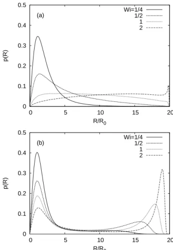
inter-mediate extensions and the above scenario becomes even more relevant. The numerical simulations of the FENE model for Rmax/R0= 20 show that, for short-correlated flows

(Ku ¿ 1), the coil–stretch transition manifests through the gradual widening of p(R) and the displacement of its maximum from values close to R0 towards values close to Rmax

(see figure 5, panel (a)). This behaviour is in agreement with the theoretical prediction for the δ-correlated isotropic flow (Martins Afonso & Vincenzi 2005) and with recent experimental measurements of polymer elongation in a random shear flow (Liu & Stein-berg 2010). For long-correlated flows (Ku & 1), the dependence of p(R) on Wi is very

(9)

1 10-1 10-2 10-3 10-4 103 102 10 1 10-1 p(R) R/R₀ R-1 Wi=1/4 1/2 1 1 10-1 10-2 10-3 10-4 103 102 10 1 10-1 p(R) R/R₀ R-1

Figure 4. PDFs of polymer elongation for the FENE model at various values of Wi in a long-correlated flow (Ku = 10). The maximum extension is set to Rmax= 103_R_0.

different. In this case, increasing Wi at fixed Ku rather produces the drop of the peak at R0 and the simultaneous formation of a second peak near Rmax (see figure 5, panel

(b)). The PDF of the extension is bimodal and the two maxima are clearly distinct: intermediate extensions are much less likely than in the small-Ku case.

The shape of p(R) for large Ku can be explained intuitively as follows. If the Lagrangian correlation time of the velocity gradient is long, a typical trajectory of a polymer is composed of long portions where the gradient can be thought as frozen with a fixed direction of stretching. Some of those portions will be characterised by a weak stretching rate, some by a strong one. The response of the polymer to the velocity gradient along one of those portions of the trajectory will be similar to the response that a polymer would have in an extensional flow with strain rate comparable to the stretching rate. As mentioned earlier, the PDF of R in an extensional flow has a sharp peak either at small extensions or at long extensions depending on the strain rate, and intermediate extensions are very unlikely. Therefore, the evolution of an isolated polymer at large Ku consists of a sequence of long deformation events, whose intensity can produce either a coiled or a highly stretched extension, whence the bimodal shape of p(R).

5. Conclusions

We have studied the influence of long temporal correlations on the dynamics of a Hookean dumbbell and of a FENE dumbbell in a two dimensional random renewing flow. The time correlation of this simple model flow can be changed arbitrarily, and this property enabled us to obtain semi-analytic predictions for the Kubo-number dependence of the statistics of polymer elongations. It is known that the PDF of the elongation of Hookean dumbbells is characterised by a power-law tail and that this power law also describes the behavior of the PDF of FENE dumbbells at intermediate elongations. We have shown that in the long-correlated limit (Ku → ∞) the power-law tail becomes almost insensitive to Wi and its slope is not an effective indicator for the coil–stretch transition. In the case of the FENE model, the long temporal correlations strongly affect the shape of the PDF, which shows two distinct maxima corresponding to the coiled and stretched configurations. For Ku À 1 we have found a new scenario for the coil–stretch

(10)

Deformation of a polymer in a random flow with long correlation time 9 0 0.1 0.2 0.3 0.4 0.5 0 5 10 15 20 p(R) R/R₀ (a) Wi=1/41/2 1 2 0 0.1 0.2 0.3 0.4 0.5 0 5 10 15 20 p(R) R/R₀ (b) Wi=1/41/2 1 2

Figure 5. PDFs of polymer elongation, p(R), for the FENE model, at various Wi numbers, in a short-correlated flow (Ku = 10−2_{, panel (a)) and in a long-correlated flow (Ku = 10, panel}

(b)). The maximum extension is fixed to Rmax= 20R0.

transition, which occurs through the drop of the peak at R0 and the simultaneous rise

of the second peak near Rmax.

Our findings can be understood in terms of basic properties of long-correlated flows, and the underlying mechanisms does not rely on the peculiar choice of the model flow used in our study. It is therefore arguable that the phenomena discussed here could be observed also in realistic flows. In particular, it would be interesting to investigate by means of numerical simulations or experimental measurements whether the presence of long-lived structures in high-Reynolds-number flows could result in the appearence of the two-peak coil–stretch transition scenario depicted here.

We are grateful to Antonio Celani and Prasad Perlekar for fruitful discussions. REFERENCES

Bagheri, F., Mitra, D., Perlekar, P. & Brandt, L. 2010 Statistics of polymer extensions in turbulent channel flow. arXiv:1011.3766v1 [physics.flu-dyn]

Balkovsky, E., Fouxon, A. & Lebedev, V. 2000 Turbulent dynamics of polymer solutions.

(11)

Bird, R. B., Hassager, O., Armstrong, R. C. & Curtiss, C. F. 1977 Dynamics of Polymeric

Liquids, vol. II. Wiley.

Boffetta, G., Celani, A. & Musacchio, S. 2003 Two-dimensional turbulence of dilute poly-mer solutions. Phys. Rev. Lett. 91, 034501.

Celani, A., Musacchio, S. & Vincenzi, D. 2005 Polymer transport in random flow. J. Stat.

Phys. 118, 531–554.

Chertkov, M. 2000 Polymer stretching by turbulence. Phys. Rev. Lett. 84, 4761–4764. Chertkov, M., Falkovich, G., Kolokolov, I. & Lebedev, V. 1996 Theory of random

advection in two dimensions. Int. J. Mod. Phys. B 10, 2273–2309.

Childress S. & Gilbert A. D. 1995 Stretch, twist, fold: the fast dynamo. Springer.

Crisanti, A., Paladin, G. & Vulpiani, A. 1993 Products of Random Matrices in Statistical

Physics. Springer.

Davoudi, J. & Schumacher, J. 2006 Stretching of polymers around the Kolmogorov scale in a turbulent shear flow. Phys. Fluids 18, 025103.

de Gennes, P. G. 1974 Coil–stretch transition of dilute flexible polymer under ultra-high velocity gradients. J. Chem. Phys. 60, 5030–5042.

Eckhardt, B., Kronj¨ager, J. & Schumacher, J. 2002 Stretching of polymers in a turbulent environment. Comp. Phys. Commun. 147, 538–?.

Frisch, U. 1995 Turbulence: The Legacy of A.N. Kolmogorov. Cambridge University.

Gerashchenko, S., Chevallard, C. & Steinberg, V. 2005 Single polymer dynamics: coil– stretch transition in a random flow. Europhys Lett. 71, 221–227

Gilbert, A. D. & Bayly B. G. 1992 Magnetic field intermittency and fast dynamo action in random helical flows. J. Fluid Mech. 241, 199–214.

Groisman, A. & Steinberg, V. 2001 Stretching of polymers in a random three-dimensional flow. Phys. Rev. Lett. 86, 934–937.

Honeycutt, R. L. 1992 Stochastic Runge–Kutta algorithms. I. White noise. Phys. Rev. A, 45, 600–603.

Larson, R. G. 2005 The rheology of dilute solutions of flexible polymers: Progress and problems.

J. Rheol. 49, 1–70.

Liu, Y. & Steinberg, V. 2010 Stretching of polymer in a random flow: Effect of a shear rate.

EPL. 90, 44005.

Lumley, J. L. 1972 On the solution of equations describing small scale deformation. Symp.

Math. 9, 315–334.

Lumley, J. L. 1973 Drag reduction in turbulent flow by polymer additives. J. Polymer Sci.:

Macromolecular Reviews 7, 263–290.

Martins Afonso, M. & Vincenzi, D. 2005 Nonlinear elastic polymers in random flow. J.

Fluid Mech. 540, 99–108.

¨

Ottinger, H. C. 1996 Stochastic processes in polymeric fluids. Springer.

Perkins, T. T., Smith D. E. & Chu, S. 1997 Single polymer dynamics in an elongational flow. Science 276, 2016–2021.

Shaqfeh, E. S. G. 2005 The dynamics of a single-molecule DNA in flow. J. Non-Newtonian

Fluid Mech. 130, 1–28.

Thiffeault, J. L. 2003 Finite extension of polymers in turbulent flow. Phys. Lett. A 308, 445–450.

Watanabe, T. & Gotoh, T. 2010 Coil–stretch transition in an ensemble of polymers in isotropic turbulence. Phys. Rev. E 81, 066301.

Zel’dovich, Ya. B., Ruzmaikin, A. A., Molchanov, S. A. & Sokoloff, D. D. 1984 Kine-matic dynamo problem in a linear velocity field. J. Fluid Mech. 144, 1–11.