Geomechanics to solve geological structure issues: forward, inverse and restoration modeling

HAL Id: tel-00537899

https://tel.archives-ouvertes.fr/tel-00537899

Submitted on 19 Nov 2010

HAL is a multi-disciplinary open access archive for the deposit and dissemination of sci-entific research documents, whether they are pub-lished or not. The documents may come from teaching and research institutions in France or abroad, or from public or private research centers.

L’archive ouverte pluridisciplinaire HAL, est destinée au dépôt et à la diffusion de documents scientifiques de niveau recherche, publiés ou non, émanant des établissements d’enseignement et de recherche français ou étrangers, des laboratoires publics ou privés.

Geomechanics to solve geological structure issues:

forward, inverse and restoration modeling

Frantz Maerten

To cite this version:

Frantz Maerten. Geomechanics to solve geological structure issues: forward, inverse and restoration modeling. Geophysics [physics.geo-ph]. UNIVERSITE MONTPELLIER II SCIENCES ET TECH-NIQUES DU LANGUEDOC, 2010. English. �tel-00537899�

UNIVERSITE MONTPELLIER II

SCIENCES ET TECHNIQUES DU LANGUEDOC

THESE

pour obtenir le grade de

DOCTEUR DE L’UNIVERSITE MONTPELLIER II

Discipline : Structure et ´

evolution de la lithosph`

ere

Ecole doctorale : SIBAGHE

pr´esent´ee et soutenue publiquement

par

Frantz MAERTEN

Le 17 juin 2010

Titre :

Geomechanics to solve geological structure

issues: forward, inverse and restoration

modeling

JURY:

M. Jean Ch´

ery

U. Montpellier, France Directeur de th`ese

M. David D. Pollard U. Stanford, USA

Codirecteur de th`ese

M. Bruno L´

evy

INRIA, France

Rapporteur

M. Yves Leroy

ENS Paris, France

Rapporteur

M. Xavier Legrand

Repsol, Madrid

Examinateur

M. Marc Daigni`

eres

U. Montpellier, France Examinateur

R´ESUM´E

Utilisation de la g´eom´ecanique pour r´esoudre des probl`emes li´es aux structures g´eologiques: mod´elisation directe, inversion et restauration Diff´erentes applications de l’´elasticit´e lin´eaire en g´eologie structurale sont pr´esent´ees dans cette th`ese `a travers le d´eveloppement de trois types de codes num´eriques. Le premier utilise la mod´elisation directe pour ´etudier les d´eplacements et champs de contraintes au-tour de zones faill´ees complexes. On montre que l’ajout de contraintes in´egalitaires, telles que la friction de Coulomb, permet d’expliquer l’angle d’initiation des dominos dans les re-lais extensifs. L’ajout de mat´eriaux h´et´erog`enes et d’optimisations, telles la parall´elisation sur processeurs multi-cœurs ainsi que la r´eduction de complexit´e des mod`eles, permettent l’´etude de mod`eles beaucoup plus complexes. Le second type de code num´erique utilise la mod´elisation inverse, aussi appel´ee estimation de param`etres. L’inversion lin´eaire de d´eplacements sur les failles ainsi que la d´etermination de pal´eo-contraintes utilisant une approche g´eom´ecanique sont d´evelopp´ees. Le dernier type de code num´erique concerne la restauration de structures complexes pliss´es et faill´ees. Il est notamment montr´e qu’une telle m´ethode permet de v´erifier l’´equilibre de coupes g´eologiques, ainsi que de retrouver la chronologie des failles. Finalement, nous montrons que ce mˆeme code permet de lisser des horizons 3D faill´es, pliss´es et bruit´es en utilisant la g´eom´ecanique.

MOTS-CL´ES: G´eologie structurale, ´elasticit´e lin´eaire, mod´elisation directe, inversion, restauration

ABSTRACT

Geomechanics to solve geological structure issues: forward, inverse and restoration modeling

Different applications of linear elasticity in structural geology are presented in this the-sis through the development of three types of numerical computer codes. The first one uses forward modeling to study displacement and perturbed stress fields around com-plexly faulted regions. We show that incorporating inequality constraints, such as static Coulomb friction, enables one to explain the angle of initiation of jogs in extensional relays. Adding heterogeneous material properties and optimizations, such as paralleliza-tion on multicore architectures and complexity reducparalleliza-tion, admits more complex models. The second type deals with inverse modeling, also called parameter estimation. Linear slip inversion on faults with complex geometry, as well as paleo-stress inversion using a geomechanical approach, are developed. The last type of numerical computer code is dedicated to restoration of complexly folded and faulted structures. It is shown that this technique enables one to check balanced cross-sections, and also to retrieve fault chronol-ogy. Finally, we show that this code allows one to smooth noisy 3D interpreted faulted and folded horizons using geomechanics.

KEYWORDS: Structural geology, linear elasticity, forward modeling, inverse modeling, restoration modeling

“Imagination is more important than knowledge”

Preface

This thesis is comprised of work that started a while ago, when I was unemployed after a bachelor degree in geophysics and geology at the University of Montpellier II. It has been continued at Stanford University within the research group of Pr David D. Pollard for four years, mainly on correcting, rewriting, enhancing and optimizing an existing 3D boundary element code. Then, several publications have emerged while at Igeoss, a start-up that we created in 2004 in Montpellier with my brother Laurent (who did his PhD with Pr David Pollard), and David Pollard himself.

After my return to France from Stanford to start Igeoss, the idea of doing a PhD came to my mind when I realized that a VAE (”valorisation des acquis et de l’experience” which can be translated to ”appreciation of achievements and experiences”) was now possible in France to obtain the equivalent of a master degree in order to start a PhD. Marc Daigni`eres, a professor at the University of Montpellier II, successfully supported my request against a faculty commitee and I was able to start in November 2006, under the direction of Jean Chery (France) and Dave Pollard (USA).

Walking in the world of geomechanics, numerical methods, optimizations and program-ming without any knowledge and background is not so simple, but can lead to new insights with the help of the imagination (hence the quote of this thesis). Eleven papers are pre-sented and one is in the appendix, which show the usefulness of linear elasticity. Although during this period three other papers were published (see appendix C), I do not include them within this thesis as I was only a little bit involved.

I particularly show in this thesis that using the simple conceptual model of linear elasticity can lead to many application codes which are used to better understand geological struc-tures using either forward, inverse or restoration modeling. The large number of publica-tions using such codes by researchers around the world (more than one hundred twenty), demonstrates their importance. A complete list of publications in different geological do-mains can be obtained on the Igeoss support website at https://support.igeoss.com.

Doing this thesis was the opportunity to start the company Igeoss in 2004 in Montpellier, and to continue the research on iBem3D, Dynel2D and Dynel3D while giving 13 inter-national conferences and writing 11 papers as well as a patent for the estimation of the state of stress in complex reservoirs using measures from well bores and faults geometry.

Finally, Igeoss integrated Schlumberger, the world’s leading supplier of technology in the oil and gas industry worldwide, after the acquisition in April 2010.

Acknowledgments

I wish to thanks, first, Dave Pollard who gently guided me in the comprehension of structural geology and geomechanics while at Stanford University. He accepted to take me in his Rock Fracture Project (RFP) group while I was programming graphical interfaces in a small company in Montpellier, and without any knowledge in numerical codes and geomechanics. I think that his choice was mainly motivated by the fact that (1) Laurent, my brother, was already working with him as a ’very good’ PhD student, and that (2) during my free time in France, I was coding a new numerical code in 2D and 3D, namely Dynel. My brother Laurent is also greatly acknowledged, and it is still a pleasure to work together: him, the structural geologist, and me the analytical geologist.

While at Stanford University (USA) and in Montpellier (FRANCE), I met many stu-dents, researchers and people from the industry who provided me a diversity of view-points in the domains of structural geology, geophysics and computer sciences. They include (alphabetical ordered): Fabrizio Agosta, Marco Antonellini, Atilla Aydin, Taixu Bai, Loic Bazalgette, Nicolas Bellahsen, Stephan Bergbauer, Stephan Bourne, Jean Ch´ery, Michele Cooke, Juliet Crider, Marc Daigni`eres, Nick Davatzes, Russell Davies, Guil-laume Deconchy, Guilhen De Joussineau, Xavier Du-Bernard, Peter Eichhubl, Patricia Fiore, Eric Flodin, Juan Mauricio Florez, Paul Gillespie, Radu Girbacea, Brita Gra-ham, Paul Griffiths, Joel Ita, Herv´e Jourde, Simon Kattenhorn, Ole Kaven, Sotiris Kokkalas, S´ebatien Lacase Serge Lallemand, Xavier Legrand, Bruno Levy, Lidia Lon-ergan, Michel Lopez, Peter Lovely, Stephen Martel, Maurice Mattauer, Matteo Molinaro, Jordan Muller, Ovunc Multu, Rodrick Myers, Ian Mynatt, Fabien Pauget, Jean-Pierre Pe-tit, Jean-Christophe Perez, Phil Resor, Paul Segall, Michel Seranne, Roger Soliva, Kurt

Sternlof, Lans Taylor, Haiquing Wu, Scott Young, Amgad Younes, Wenbing Zhang, Marc Zoback, and certainly many other people...

I thanks people who accepted to review this work in a short time: Bruno Levy and Yves Leroy, as well as the “examinateurs”: Xavier Legrand, Loic Bazalgette (Shell) and Marc Daigni`eres. And, of course, my principal advisor, Jean Chery, from the University of Montpellier II.

Many thanks to Roger Soliva from the University of Montpellier who helped me to un-derstand some geological features in the field, and who provided helpful feedback before the PhD defense. It is always a great pleasure to discuss “structural geology” with him. I also thanks the Igeoss team for the hard work they provided: Alexandre Baranov, Jean-Pierre Joonnekindt, Dieter Knoll, Thomas Laverne, Fran¸cois Lepage, Frederic Marmond, Michael Palomas, Emanuel Quetelard, and especially David Desmarest who teach me the object oriented languages while at “After Development” in Montpellier. He was my mentor and is now a precious element at Igeoss.

Igeoss consortium members are acknowledged for their support in the development of iBem3D, Dynel2D and Dynel3D: BG-Group, BhpBilliton, Chevron, ConocoPhillips, Eni, ExxonMobile, Repsol, Shell and Total.

People from the CEEI, LRI and the “Region Languedoc Roussillon” are also acknowl-edged: Josick Paoli (R´egion Languedoc Roussillon) who trusted and helped us to start Igeoss, the team of Cap Alpha and Cap Omega, the team of LRI and especially G´eraldine Karbouch, Jean-Paul Mikallef from Transfert LR.

Noel Lichau is also acknowledged. He helped me to discover the structural geology while doing speleology.

Many thanks to my father and mother in law, Freddy and Eliane Genieys, who helped me to find an equilibrium during these hard years, and with whom I use to rock climb. Finally, I thanks my wife and my children for their patience and comprehension during these hard years of continuous work: Claire, Lila and Tristan. Claire is a very precious help.

By the way, I do not recommend to start a company and to do a PhD thesis while working for that company, remodeling an old house, having 2 babies during that time, taking care of 150 olive trees, giving free math courses for families with no resources and being in charge of starting a Geosciences cluster in the R´egion Languedoc Roussillon. Good luck

CONTENTS

Preface. . . 4

Acknowledgments . . . 6

Table of contents . . . 9

Introduction . . . 17

I

Forward modeling using Boundary Element Method

23

Aper¸cu. . . 24

Overview . . . 25

1 iBem3D, a three-dimentional iterative boundary element method using angular dislocations for sub-surface structures modeling 27 Preamble . . . 27

1.1 R´esum´e . . . 30

1.2 Abstract . . . 31

1.3 Introduction . . . 31

1.4 Theory behind iBem3D . . . 33

1.4.1 Angular, biangular and triangular dislocations . . . 35

1.4.2 Element boundary conditions . . . 39

1.4.3 Remote loading . . . 40

1.4.4 Post-processing at observation points . . . 41

1.4.5 Benchmarking the code. . . 41

1.5 Enhancements to iBem3D . . . 45

1.5.1 Heterogeneous material . . . 45

1.5.2 Friction and non-interpenetration . . . 45

1.5.3 Linear slip inversion . . . 46

1.5.4 Paleostress. . . 46

1.5.5 Optimization . . . 47

1.6 Applications . . . 47

1.6.1 Research and Academic applications . . . 48

1.6.1.1 Teaching . . . 48

1.6.1.3 Structural geology . . . 48

1.6.1.4 Active tectonics and earthquakes . . . 50

1.6.1.5 Volcanoes . . . 51

1.6.2 Industry and engineering applications . . . 53

1.6.2.1 Subsurface fault interpretation . . . 53

1.6.2.2 Subsurface small-scale fracture modeling . . . 53

1.6.2.3 Perturbed stress field and fracture reactivation . . . 54

1.6.2.4 Risk assessment. . . 55

1.7 Conclusions . . . 56

1.8 Acknowledgments . . . 56

1.9 Appendix: Shadow effect correction . . . 66

1.9.1 Description of the problem . . . 66

1.9.2 Solution of the problem . . . 67

1.9.2.1 Corrective displacement for observation points . . . 67

1.9.2.2 Corrective displacement for triangular elements . . . 69

2 Solving 3D boundary element problems using constrained iterative ap-proach 70 Preamble . . . 70 2.1 R´esum´e . . . 72 2.2 Abstract . . . 73 2.3 Introduction . . . 73 2.4 System definition . . . 75

2.4.1 Boundary Element formulation . . . 77

2.4.2 Block relaxation scheme . . . 79

2.5 Performance . . . 81

2.6 Convergence . . . 83

2.7 Inequality constraints . . . 83

2.7.1 Frictionless contact . . . 84

2.7.1.1 Verification . . . 86

2.7.2 Static Coulomb friction. . . 88

2.7.2.1 Verification with a 2D analytical solution . . . 89

2.7.2.2 Comparison with the penalty method. . . 91

2.7.2.3 Model 1 . . . 92

2.7.2.4 Model 2 . . . 92

2.7.3 Effect of an incremental remote loading . . . 96

2.8 Conclusion . . . 97

2.9 Acknowledgements . . . 98

2.10 Appendix . . . 98

3 Field evidences for the role of static friction on fracture orientation in extensional relays along strike-slip faults; comparison with photoelastic-ity and 3D numerical modeling 104 Preamble . . . 104

3.1 R´esum´e . . . 107

3.3 Introduction . . . 108

3.4 Field data . . . 111

3.4.1 Geological setting . . . 111

3.4.2 Extensional relay geometries . . . 113

3.5 Photoelastic modeling . . . 116

3.5.1 Photoelastic method . . . 116

3.5.2 Experimental results of extensional relay stress pattern . . . 117

3.6 Numerical modeling. . . 119

3.6.1 Model set up . . . 120

3.6.2 Modeling of joints reactivated in shear . . . 120

3.6.3 Modeling of stylolite reactivated in shear . . . 121

3.6.4 Parametric analysis . . . 121

3.7 Discussion . . . 125

3.7.1 Stress perturbation and friction of the slipping defects. . . 125

3.7.2 Estimation of fault friction and upscaling . . . 126

3.8 Conclusion . . . 127

3.9 Acknowledgments . . . 128

4 Iterative 3D BEM solver on complex faults geometry using angular dis-location approach in heterogeneous, isotropic elastic whole or half-space134 Preamble . . . 134 4.1 R´esum´e . . . 136 4.2 Abstract . . . 137 4.3 Introduction . . . 137 4.4 BEM formulation . . . 138 4.5 Iterative solver . . . 140 4.6 Results . . . 142 4.7 Optimizations . . . 143

4.7.1 Bufferized elemental matrices . . . 143

4.7.2 Parallelization on multi-core processors . . . 143

4.8 Conclusions . . . 144

5 Adaptive cross approximation applied to system resolution and post-processing for a 3D elastostatic problem using the Boundary Element Method 146 Preamble . . . 146

5.1 R´esum´e . . . 149

5.2 Abstract . . . 150

5.3 Introduction . . . 150

5.4 Boundary Element formulation . . . 151

5.5 Blockwise low-rank approximant. . . 155

5.5.1 _H-Matrices . . . 156

5.5.2 ACA . . . 157

5.6 H-Matrices applied to the resolution of the system of equations . . . 157

5.7 H-Matrices applied to post-processing at observation points . . . 159

5.7.2 Example . . . 161

5.7.3 Effect of field points distribution . . . 164

5.8 Parallelization on multi-core CPU . . . 166

5.8.1 Example . . . 168

5.9 Conclusions and perspectives. . . 169

5.10 Acknowledgments . . . 170

II

Inverse modeling using Boundary Element Method

173

Aper¸cu. . . 174

Overview . . . 175

6 Inverting for Slip on Three-Dimensional Fault Surfaces using Angular Dislocations 176 Preamble . . . 176 6.1 R´esum´e . . . 178 6.2 Abstract . . . 179 6.3 Introduction . . . 179 6.4 Method . . . 181

6.5 Application to the 1999 Hector Mine Earthquake . . . 185

6.5.1 Modeling . . . 187

6.5.2 Results . . . 190

6.6 Discussion and Conclusions . . . 194

6.7 Acknowledgements . . . 195

7 Co- and post-seismic deformation of the 28 March 2005 Nias Mw 8.7 earthquake from continuous GPS data 201 Preamble . . . 201

7.1 R´esum´e . . . 203

7.2 Abstract . . . 204

7.3 Introduction . . . 204

7.4 Co- and Postseismic Displacements . . . 205

7.5 Co- and Postseismic Slip Model . . . 207

7.6 Discussion and Conclusions . . . 208

7.7 Acknowledgments . . . 209

8 Mechanical analysis of fault slip data 213 Preamble . . . 213

8.1 R´esum´e . . . 215

8.2 Abstract . . . 216

8.3 Introduction . . . 216

8.4 Accounting for a Complete Mechanics . . . 221

8.5 Test Results for Stress Inversion . . . 226

8.5.1 Heuristic Example: Single Fault Inversions . . . 226

8.5.2 Heuristic Example: Fault System with Diverse Orientations . . . . 231

8.6 Conclusions . . . 239

9 Applications of the principle of superposition for paleo-stress analysis and fault modeling 249 Preamble . . . 249

9.1 R´esum´e . . . 252

9.2 Abstract . . . 253

9.3 Introduction . . . 253

9.3.1 Generation 1: Anderson’s inversion for tectonic stress regimes . . . 254

9.3.2 Generation 2: inversion using slickenlines or focal mechanisms . . . 256

9.3.3 Generation 3: inversion using heterogeneous stress fields . . . 258

9.4 Theory . . . 261

9.4.1 Modeling using iBem3D . . . 261

9.4.2 Reduced far field stress tensor . . . 262

9.4.3 Principle of superposition . . . 264

9.4.4 Complexity estimate . . . 264

9.5 Real time computation . . . 265

9.6 Paleostress inversion using field measurements . . . 266

9.6.1 Method of resolution . . . 266

9.6.2 Geologic, geophysical, and geodetic data sets . . . 267

9.6.2.1 Data sets containing only orientation information . . . 268

Using fractures and stylolites orientations . . . 268

Example: Nash Point (UK) . . . 269

Using secondary fault planes . . . 270

Example 1: Normal and thrust fault . . . 270

Example 2: Oseberg-Syd (Norway) . . . 270

Using fault striations . . . 273

9.6.2.2 Data sets containing magnitude information . . . 274

Using GPS data . . . 274

Using InSAR data . . . 275

Example . . . 275

Using flattened horizon . . . 275

Example . . . 275

Using dip-slip information . . . 276

9.6.2.3 Using all available information . . . 277

9.7 Multiple tectonic events . . . 278

9.7.1 Example . . . 278

9.8 Seismic interpretation quality control . . . 280

9.9 Conclusion and perspectives . . . 281

9.10 Acknowledgments . . . 281

III

Structural restoration using Finite Element Method

287

Aper¸cu. . . 288

10 Chronologic modeling of faulted and fractured reservoirs using

geomechanically-based restoration: Technique and industry applications 290

Preamble . . . 290

10.1 R´esum´e . . . 293

10.2 Abstract . . . 294

10.3 Introduction . . . 294

10.4 Principles and Method . . . 297

10.4.1 Principles . . . 298

10.4.2 Method . . . 298

10.5 Application to restoration and example tests . . . 301

10.5.1 Model configurations . . . 301

10.5.2 Results . . . 302

10.6 Experiment 1 . . . 304

10.6.1 Numerical model configuration . . . 305

10.6.2 Restoration results . . . 307

10.6.3 Fault development analysis. . . 309

10.6.4 Active deformation area . . . 311

10.6.5 Fault propagation . . . 311

10.6.6 Locking faults . . . 313

10.6.7 Fault chronology . . . 313

10.6.8 Conclusions and applications to reservoir exploration and production313 10.7 Experiment 2 . . . 314

10.7.1 Numerical model configuration . . . 314

10.7.2 Restoration results . . . 314

10.7.3 Conclusions and applications to reservoir exploration and production317 10.8 Experiment 3 . . . 318

10.8.1 Numerical model configuration . . . 319

10.8.2 Restoration results . . . 321

10.8.3 Conclusions and applications to reservoir exploration and production322 10.9 Conclusions . . . 322

10.10Acknowledgments . . . 325

11 Geomechanically smoothing noisy horizons 331 Preamble . . . 331

11.1 R´esum´e . . . 333

11.2 abstract . . . 334

11.3 Introduction . . . 334

11.4 Features classification. . . 336

11.5 Iterative FEM method . . . 340

11.5.1 Determination of the element and nodal deformation . . . 340

11.5.2 Contacts at interfaces. . . 341

11.5.3 Solving the system . . . 342

11.6 Geomechanical smoothing filter . . . 343

11.7 Verifications . . . 345

11.7.1 Bumps . . . 345

11.7.3 Wavy fault cut-off. . . 346

11.8 Application . . . 346

11.8.1 Local surface correction . . . 347

11.8.2 Extending fault tips . . . 355

11.9 Conclusions . . . 356

IV

Conclusions and perspectives

358

V

Appendices

363

A Fast iterative slip inversion 365 A.1 R´esum´e . . . 367

A.2 Abstract . . . 368

A.3 Introduction . . . 368

A.4 BEM formulation . . . 369

A.4.1 Iterative formulation . . . 370

A.4.2 Tikhonov regularization . . . 371

A.4.3 Solving the system with inequality constraints . . . 372

A.5 Reducing the model complexity . . . 373

A.5.1 H-Matrices . . . 374

A.5.2 ACA . . . 375

A.5.3 Applying H-Matrix and ACA to the system construction . . . 375

A.5.3.1 Model partitioning . . . 376

A.5.3.2 Fast evaluation of AT_{WA for an element e . . . 377}

A.5.3.3 Fast evaluation of AT W(d − c) for an element e . . . 377

A.6 Conclusions . . . 378

A.7 Appendix: Tikhonov regularization in the normal equation . . . 381

B Fault reactivation and fault properties: 3D geomechanical modeling ap-proach and application to nuclear waste disposal 382 B.1 R´esum´e . . . 383

B.2 Abstract . . . 384

B.3 Introduction . . . 384

B.4 Methodology . . . 384

B.5 Example case study . . . 385

B.6 Model configuration. . . 385

B.7 Model results analysis . . . 386

B.8 Conclusions . . . 387

C Other publications and conferences 389 C.1 Other international publications . . . 390

C.2 Rock Fracture Project abstracts, Stanford, CA . . . 392

C.3 Conference abstracts . . . 393

Introduction

Physical theories always deal with simplifications of nature, simply because modeling a complicated structure such as the earth at a large scale using a microscopic atomistic molecular model is unrealistic. Therefore, researchers tend to capture the most important properties of real objects, and use them in a conceptual theoretical, then analytical and numerical model, the goals being to explain and predict physical phenomena.

We can distinguish two types of physical models that provide foundations for all physi-cal theories for modeling the material behavior: (1) microscopic discrete models, and (2) macroscopic continuum models. At the microscopic scale, the particles are moving ac-cording the influence of their mutual interaction forces given by the quantum mechanics. At a much larger scale, objects are governed by continuum theories (solid mechanics, fluid mechanics, elasticity, thermodynamics, electromagnetism, acoustic, and so forth). These theories tend to describe the behavior of objects in our perception of four dimensional space-time. Matter and energy are considered as a continuum in this framework, and therefore mathematical representation of physical quantities is by means of continuous (or piecewise continuous) functions of space and time.

These kind of problems can be solved exactly by mathematical manipulations (analytical models), but the mathematical tools usually limit the possibilities to oversimplified mod-els. Therefore, various techniques of discretization have been proposed and developed, leading to numerical models involving approximation that approach the true analytical solution as the number of discrete variables increases. The goal of these methods is to numerically solve the partial differential equations (PDE). Well known methods are the Finite Difference Method (FDM), the Finite Element Method (FEM) and the Boundary Element Method (BEM).

The FDM is the earliest classical numerical treatment for solving PDE, and it replaces the continuum solution by a set of lattice points. At each point, any differential operators are replaced by finite difference operators, leading to a set of difference equations which can be easily solved.

In FEM, the solution domain is discretized into a number of uniform or nonuniform finite elements that are connected by mean of nodes, and the change in the dependent variable with regard to location is approximated within each elements using a shape function. The BEM uses the fact that equations in differential forms can often be transformed into integral forms. It transforms the differential operator defined in the domain into an inte-gral operator defined on the boundary. Hence, in BEM, only the boundary of domains of interest need to be discretized.

discretized, and a mesh is needed. In BEM, only the bounding surfaces (in 3D) are used. The focus of this thesis is the continuum mechanics applied to the comprehension of geological phenomena, using partial differential equation-based (PDE) modeling with boundary conditions. More precisely, we are interested in quasi-static phenomena (e.g. co-seismic events) in the sub-surface using linear elasticity, which proves to be a good approximation and can provide new insights for the comprehension of earthquakes and volcanoes or to study the state of perturbed stress field around a complexly faulted area.

Three kind of numerical codes are developed: (1) forward modeling, (2) inverse modeling and (3) restoration modeling.

1. Forward modeling studies the fault response to an imposed far field stress or strain given the fault geometry and the boundary conditions. Result of such simulations can be used, for example, to predict fractures due to faulting, or to study fault triggering in an earthquake process.

2. Inverse modeling is a form of parameters estimation of what is usually imposed or computed on faults in the forward sense (i.e. far field stress, fault slip distribution). Given some observed deformation at Earth’s surface due to faulting at depth, the aim is to invert for the slip distribution onto the faults that induced such observed displacements, or to invert for a tectonic loading (also called paleostress in the literature) which activated the faults which, in turn, generated the deformations at the ground surface.

3. Restoration modeling is the study of the geological structures (geometry) back in time using special boundary conditions onto a model which are related to geological phenomena (e.g. sedimentation, erosion). This type of modeling allows one, for example, to validate the structural interpretation of geological structures, to pre-dict fractures due to folding, or to determine the faults chronology as we go back in time. It is also used to localize and correct anomalous zones of high stress/s-train concentration on 3D faulted and folded horizons, and therefore, operates has a geomechanically-based smoothing filter.

Contents of the thesis

This thesis is divided into three main parts containing a total of eleven papers that are either published, submitted or in preparation. Another paper in preparation is presented in appendix, which complete the work done during this thesis.

Part I is devoted to forward modeling using an elastostatic Boundary Element Method (BEM) called iBem3D (the successor of Poly3D originally developed at Stanford Univer-sity), and is composed of five chapters. We show, in this first part of the thesis, that the conceptual model using the boundary element method can be extended to incorporate (i) preventing of element interpenetration while allowing opening mode (ii) the static friction with varying friction coefficient and cohesion, and (iii) the material heterogeneity using complex shaped interfaces between regions of different material properties. A special chapter is devoted to the optimization and parallelization of such a code, which is useful for modeling material heterogeneity. Finally, a chapter applies the static friction to the study of fracture orientation in extensional relays.

Part II of this thesis studies the inverse modeling using the same boundary element code, and is subdivided in three chapters related to (i) slip inversion, (ii) paleostress estimation and (iii) slip recovery. A chapter is devoted to the application of the slip inversion applied to the Nias earthquake (Indonesia). Appendix A presents an optimization technique of the slip inversion using the procedures described in part I.

Part III uses another numerical method, namely the Finite Element Method (FEM), to restore structural interpretations for validation or prediction of fractures related to folding (chapter 10). Chapter 11 also presents another application to restore 3D surfaces (unfaulting and unfolding simultaneously) in order to localize anomalous geometries. It proposes an algorithm to correct for the initial geometry by minimizing a user selected criteria (e.g. stress, strain, area change, ...). These two tools are very useful for the correc-tion of faults geometry before doing any forward or inverse modeling using the boundary element codes presented in part I and II.

Part I

: forward modeling using linear elasticity with a boundary element code.

Chapter

1

presents the foundation of this thesis. We show that using the analytical formulation of the displacement field induced by an angular disloca-tion in a homogeneous elastic whole- or half-space, it is possible to construct 3D complex surfaces of displacement discontinuity made of triangular elements. This formulation allows surfaces of discontinuity to have complex shapes and tip-lines, as opposed to Okada’s formulation, currently the standard method in

geophysics, where rectangular elements are used inducing inevitably overlaps and gap between the elements. Application of such a code is wide in the do-mains of structural geology and geomechanics. We present some of the major applications that have already been published by a large community around the world.

Chapter

2

proposes an iterative method to solve the system of linear equa-tions. This technique allows one to reduce the model complexity from O(n3_),

while using the Gauss elimination or LU decomposition, to O(kn2_{), where}

k is the number of iterations required for the iterative solver. Moreover, this solver allows the incorporation of inequality constraints on traction (e.g. static Coulomb friction) and displacement (e.g. non-interpenetration of the elements). As we will see, it also facilitates the parallelization on multi-core architectures.

Chapter

3

presents an application of the inequality constraints from chapter

2 to the orientations of branching fractures at strike slip relay zones between reactivated en echelon stylolites and joints. The chosen area is ”Les Matelles” located near Montpellier, France. Specifically, it is shown that the orientation of the domino within the relay zone is function of the friction.

Chapter

4

shows that the initial implementation of the boundary element code, which was done for an homogeneous isotropic material, can be extend to heterogeneous isotropic materials using special boundary conditions at inter-faces separating regions of different material properties. These interinter-faces are discretized as 3D triangulated surfaces that can have any shape.

Chapter

5

is devoted to the optimization of forward modeling. Even if using an iterative approach (chapter 2) decreases the model complexity, it remains a major drawback for computing large models made of hundreds of thousands triangular elements, the memory needed being the same as when using direct matrix inversion. Furthermore, the post-processing at observation grids can be a penalization for the user, especially if the number of observation points is large. This chapter presents the optimization of the computation by using approximations and parallelization on multi-core processors, for both the system resolution and post-processing. It is shown that the model com-plexity is reduced from O(kn2_{), for an iterative solver, to ∼ O(kn), and that}

the post-processing at observation points (field points) is drastically reduced and is a function of the position of the grids relative to the sources (surface discontinuities).

Part II

: Inverse modeling using linear elasticity with a boundary element code.

Chapter

6

presents the advantages of doing linear slip inversion on complex fault geometries. Given some observations of deformations at the ground sur-face (e.g. GPS, tiltmeters, satellite images, ...) as well as the fault geometries, we invert for slip distributions onto the faults that generated such measured deformations. Specifically, it is shown that such an approach using triangular elements is more precise than traditional methods using rectangular-planar el-ements. The code is applied to the Hector Mine earthquake, CA, and performs better than when using rectangular elements.

Chapter

7

presents an application of the slip inversion for the Nias earth-quake which occurred in 2005 in Indonesia. This study adds evidence that the earthquake probably did not break the surface, and this has implications for tsunami generation.

Chapter

8

presents a geomechanically-based technique to recover for the paleostress that induced observed displacements onto the faults from seismic interpretation. This technique is limited to one tectonic event, but can give a good estimate of what could have been the orientation and magnitude of the tectonic loading using mechanical interactions. While doing the stress inver-sion, we invert at the same time for the unknown displacement discontinuities onto the faults (e.g. strike-slip).

Chapter

9

presents another way of doing paleo-stress estimation using the principle of superposition that applies in linear elasticity. This new method can take into account various data sets such as fracture and secondary fault plane orientation that formed in the vicinity of active faults, GPS, InSAR, fault throw and slickenlines. It is shown that multiple tectonic events can be recovered and the data may be segregated into their respective events. Furthermore, such a method allows one to do real-time computation of the faults slip and perturbed stress field while the user changes the imposed far

Part III

: Restoration modeling using linear elasticity with a finite element code.

Chapter

10

is devoted to the validation of interpretations using a restora-tion technique. Doing forward modeling, as describe in chapter 1, shows the importance of the fault and fracture geometry to the resulting computed dis-placement discontinuity onto them, and consequently to the associated per-turbed stress field. For the majority of the numerical simulations, it is manda-tory to validate such interpretations before analyzing the result of a forward numerical simulation.

Chapter

11

presents a geomechanically-based smoothing filter for noisy 3D surfaces. It is shown that the filter removes geometrical artifacts where, for example, high stress concentration occurs after unfolding and unfaulting, while smoothing fault cut-offs and transforming high displacement gradients at crack-tips into a more realistic geometry.

Additionally, we present in appendix A, an on-going project related to part II (Inverse modeling using Boundary Element Method) for doing fast slip inversion using an iterative solver. In appendix B, we present a sensitivity analysis for fault sealing and leakage for both nuclear waste disposal and exploitation of natural resources.

Part I

Forward modeling using Boundary

Aper¸cu

La premi`ere partie de cette th`ese est consacr´ee `a la mod´elisation directe en d´eveloppant et utilisant iBem3D (ex-Poly3D), une m´ethode d’´el´ements fronti`eres (BEM). Etant donn´e la g´eom´etrie 3D des failles ainsi que le champ de contraintes `a l’infini, il est possible de d´eterminer les champs de d´eplacement et de contraintes perturb´es autour de zones complexes faill´ees (chapitre 1). Des am´eliorations de ce code sont propos´ees dans le chapitre2, o`u les contraintes in´egalitaires sont ajout´ees dans la formulation, ce qui permet de simuler la friction Coulombienne et la non-interp´en´etration des plans de failles lors d’un r´egime compressif. Dans le chapitre 3, nous donnons une application directe du frottement pour ´etudier les angles de branchement des dominos dans un relais extensif. Les am´eliorations comprennent aussi l’ajout de mat´eriaux h´et´erog`enes `a l’aide d’interfaces 3D triangul´ees s´eparant deux r´egions ayant des propri´et´es m´ecaniques diff´erentes (chapitre

4). Du fait qu’une telle am´elioration induit un accroissement non n´egligeable dans le nombre d’inconnues, des optimisations sont n´ecessaires (r´eduction de la complexit´e ainsi que parall´elisation sur des architectures multi-cœurs). Ces optimisations sont pr´esent´ees dans le chapitre 5.

L’annexe B pr´esente une utilisation ´el´egante des contraintes in´egalitaires pour l’analyse de sensibilit´e de differents param`etres. On utilise Scribble, un langage en Javascript pour iBem3D, permettant d’ex´ecuter rapidement des milliers de mod`eles. Dans cette mod´elisation, trois param`etres interd´ependants sont analys´es pour ´etudier `a la fois les risques sismiques li´es au stockage de d´echets nucl´eaires et l’exploitation des ressources naturelles: (1) l’´epaisseur de la glace au-dessus des failles, (2) la friction sur les failles et (3) la coh´esion.

Overview

The first part of this thesis is dedicated to forward modeling using iBem3D (former Poly3D), a Boudnary Element Method (BEM). Having the faults geometry as well as the far field stress, it is possible to determine the displacement and perturbed stress field around complex faulted areas (chapter 1). Enhancements of iBem3D are proposed in chapter 2, where inequality constraints are added in the formulation, allowing Coulomb frictional behavior and non-interpenetration of elements making a fault in a compressional regime. In chapter 3 we give a direct application of the friction to study the different branching angles for the initiation of the jogs in extensional relays. Enhancements also include heterogeneous materials by using complexly-shaped 3D interfaces separating two regions with different materials properties (chapter 4). Since such an extension induces a non-negligible jump in the number of unknowns, optimizations are necessary (complexity reduction as well as parallelization on multicore architectures). This is done in the chapter

5.

Appendix B presents an elegant application of the inequality constraints for sensitivity analysis. It uses Scribble, the Java-script language for iBem3D, to quickly run thousands of models. In this particular modeling, three inter-dependent parameters are analyzed for both nuclear waste disposal and exploitation of natural resources: (1) ice thickness above the faults, (2) fault friction and (3) fault cohesion.

Chapters

1 iBem3D, a three-dimentional iterative boundary element method

using angular dislocations for sub-surface structures modeling 27

2 Solving 3D boundary element problems using constrained iterative

approach 70

3 Field evidences for the role of static friction on fracture

orienta-tion in extensional relays along strike-slip faults; comparison with

photoelasticity and 3D numerical modeling 104

4 Iterative 3D BEM solver on complex faults geometry using angular

dislocation approach in heterogeneous, isotropic elastic whole or

half-space 134

5 Adaptive cross approximation applied to system resolution and

post-processing for a 3D elastostatic problem using the Boundary

CHAPTER 1

IBem3D, a three-dimentional iterative

boundary element method using angular

dislocations for sub-surface structures

modeling

F. Maerten(1,2)_{, L. Maerten}(1)_{, D. D. Pollard}(3)_{, Y. Lagalay}(4)

(1) Igeoss, Montpellier, FRANCE

(2) University of Montpellier II, Geosciences, FRANCE (3) Stanford University, CA, USA

(4) EMEA Oil & Gas Group, Paris, FRANCE To be submitted to Journal of Structural Geology

Figure 1.7 and 1.8 with permission of Journal of Structural Geology. Figure 1.9 and 1.11 with permission of Journal of Geophysical Research. Figure 1.10 with permission of Earth and Planetary Science Letters. Figure 1.12 with permission of AAPG Bulletin.

Preamble

The following chapter presents the foundation of this thesis. We show that using the analytical formulation of the displacement field induced by an angular dislocation in a homogeneous elastic whole- or half-space, it is possible to construct 3D complex surfaces of displacement discontinuity made of triangular elements. This formulation allows sur-faces of discontinuity to have complex shapes and tip-lines, as opposed to the Okada’s formulation, where rectangular elements are used inducing inevitably overlaps and gaps between the elements. Application of such a code is wide in the domains of structural geology and geomechanics. We review some of the major applications that have already been published by a large community around the world.

About...

Poly3D versus iBem3D

Historically, the development of Poly3D started in 1993, and was written at Stanford University by Andrew Lyle Thomas (Thomas, 1993) using the C language and based on the work of Jeyakumaran (Jeyakumaran et al., 1992). In 1998, Yann Lagalay came at Stanford for one year to work on the “Shadow’s effect” problem (see section 1.9). A year after, I came in the group of Dave Pollard, and started to correct some bugs, optimize the fundamental equations and rewrite the core code in pseudo C++ (C++ wrapper around the C language).

Since then, the code was entirely rewritten in C++ while at Igeoss, adopting the triangular elements instead of the more general polygonal formulation, for speed and design considerations. Several enhancements are now part of the new code, such as a fast iterative solver, parallelization on multicore architectures, H-Matrix optimization, heterogeneity of materials, inequality constraints (static friction) and paleo-stress evaluation. The new code is now named Ibem3D...

For this paper, Laurent Maerten wrote the “Applications” part while Dave Pollard enhanced the manuscript and wrote the introduction, the verification part as well as the conclusions.

Article Outline

Preamble. . . 27

1.1 R´esum´e . . . 30

1.2 Abstract . . . 31

1.3 Introduction . . . 31

1.4 Theory behind iBem3D. . . 33

1.4.1 Angular, biangular and triangular dislocations . . . 35

1.4.2 Element boundary conditions . . . 39

1.4.3 Remote loading . . . 40

1.4.4 Post-processing at observation points. . . 41

1.4.5 Benchmarking the code . . . 41

1.5 Enhancements to iBem3D . . . 45

1.5.1 Heterogeneous material . . . 45

1.5.2 Friction and non-interpenetration . . . 45

1.5.3 Linear slip inversion . . . 46

1.5.4 Paleostress . . . 46

1.5.5 Optimization . . . 47

1.6 Applications . . . 47

1.6.1 Research and Academic applications . . . 48

1.6.2 Industry and engineering applications . . . 53

1.7 Conclusions . . . 56

1.8 Acknowledgments . . . 56

1.9 Appendix: Shadow effect correction . . . 66

1.9.1 Description of the problem . . . 66

1.1

R´

esum´

e

Le but de cet article est de d´ecrire iBem3D, un code C++ modulaire bas´e sur la th´eorie des dislocations angulaires pour la mod´elisation en trois dimensions des fractures et failles dans un milieu infini ou semi-infini, ´elastique, h´et´erog`ene et isotrope. Nous pr´esentons aussi les am´eliorations apport´ees `a ce code ainsi que le grand nombre d’applications dans le domaine de la g´eologie structurale depuis la premi`ere impl´ementation en 1993 sous le nom de Poly3D. Le principal avantage d’utiliser une telle formulation pour d´ecrire les failles et fractures, r´eside dans la possibilit´e de mod´eliser des g´eom´etries complexes sans trou ni recouvrement entre les ´el´ements adjacents discontinus, ce qui est tr`es probl´ematique pour les mod`eles utilisant des dislocations rectangulaires. Fiabilit´e, vitesse de calcul, simplicit´e et exactitude des r´esultats sont am´elior´es dans la derni`ere version de ce code.

Les applications industrielles comprennent la mod´elisation des failles sous-sismiques, la mod´elisation des r´eservoirs fractur´es, l’interpr´etation et la validation de la connectivit´e des failles et de la compartimentation des r´eservoirs, l’´etude des zones d´epl´et´ees, la r´eactivation des failles et la stabilit´e des puits de forage sous pression. Les applications acad´emiques comprennent l’´etude des tremblements de terre et la surveillance des volcans, l’att´enuation des risques sismiques ainsi que la mod´elisation de stabilit´e des glissements de terrain.

1.2

Abstract

The purpose of this paper is to describe iBem3D, a C++ and modular computer pro-gram based on the theory of angular dislocations for three-dimensional fracture and fault modeling in an elastic, heterogeneous, isotropic whole- or half-space, and to present the extensions as well as the wide range of applications in structural geology since its first implementation in 1993 under the name Poly3D. The main advantage of using this for-mulation for describing faults and fractures resides in the possibility of modeling complex geometries without gaps and overlaps between adjacent triangular dislocation elements, which is a significant shortcoming for models using rectangular dislocation elements. Re-liability, speed, simplicity and accuracy are enhanced in the latest version of the computer code. Industrial applications include subseismic fault modeling, fractured reservoir mod-eling, interpretation/validation of fault connectivity and reservoir compartmentalization, depleted area and fault reactivation, and pressurized well bore stability. Academic appli-cations include earthquake and volcanoe monitoring, hazard mitigation and slope stability modeling.

Keywords: 3D-BEM, Geomechanics, Faults interaction, Sub-surface modeling

1.3

Introduction

The rapidly increasing number of geologic, seismologic and geodetic data sets with abun-dant and very precise spatial information on fault geometry and slip distributions promote the development of more complex geometric and kinematic models of modern earthquake ruptures and paleoseismic events. These data sets indicate that faults commonly are com-posed of multiple discrete segments, each with a curved surface and curved tipline. Con-struction of model fault segments using multiple rectangular dislocations (Okada, 1985) introduces non-physical gaps and overlaps with associated stress concentrations and irreg-ularities in slip distributions that may differ significantly from those in nature (Maerten

et al., 2005). Discretization of fault segments into a set of triangular dislocations enables

one to approximate the curviplanar surfaces and curved tiplines to a precision that is consistent with the data (Jeyakumaran et al.,1992;Thomas, 1993; Maerten et al., 2005,

2009; Maerten, 2010).

The C computer code that was originally developed at Stanford University by Andrew Thomas (Thomas, 1993) in 1993 was called Poly3D. The idea of using the angular dis-location formalism to construct complex planar disdis-locations with constant displacement

M. Jeyakumaran et al. (1992) - Formulation for triangular elements - Resolution using a direct solver

Figure 1.1: Poly3D versus iBem3D. Both of them are based on Comninou and Dun-durs work (Comninou and Dundurs,1975) and Jeyakumaran (Jeyakumaran et al.,1992). While Poly3D employs polygonal elements, iBem3D uses triangular elements and relies exclusively on an iterative solver. Compared to Poly3D, where the equations for the dis-placement field were symbolically derived using a computer program, iBem3D uses hand made derivatives (now running 4 times faster) and incorporates many enhancements.

Since then, due to the rapid evolution of computer power and the constant demand for doing more complex and larger models, a new code has emerged, following the work of Jeyakumaran (Jeyakumaran et al., 1992) for triangular elements. To develop the new code, iBem3D, the C++ object oriented language was chosen and an iterative solver now replaces the older direct solver (Gauss elimination). C++ allows modularity of the code (Maerten and Maerten, 2008a; Maerten et al., 2009; Maerten, 2010) while the iter-ative solver permits running larger models in a shorter time (Maerten et al., 2009). The equations for the displacement field provided by Comninou and Dundurs (Comninou and

Dundurs, 1975) were entirely derived by hand for optimization considerations, whereas

Poly3D equations were symbolically derived using a dedicated software. The call to the core equations now runs four times faster. Comparisons of Poly3D and iBem3D are sum-marized in Figure 1.1 where the technological differences are highlighted.

In this paper, we summarize the theory behind iBem3D along with verifications (sec-tion 1.4), and present the latest improvements such as the implementation of material heterogeneity, static friction, optimizations and parallelization, linear-slip inversion and paleostress recovery (section 1.5). Finally, the wide range of academic, research and in-dustrial applications are discussed in section 1.6.

1.4

Theory behind iBem3D

The theory of dislocations in elastic materials has been used widely over the past half cen-tury to evaluate the displacement, strain and stress fields around faults in Earth’s litho-sphere. Steketee discussed this theory and potential applications to geophysical problems in two papers (Steketee, 1958b,a). He reviewed Volterra’s formulation for the dislocation problem and presented a method for the construction of Green’s functions for the semi-infinite space containing a surface of displacement discontinuity (the dislocation). The Green’s functions can be integrated to calculate the displacement field around the planar surface of discontinuity. These displacement fields satisfy the Navier equations which are the governing equations for linear elastic theory. Spatial derivatives of the displacement components provide the strain components, and incorporation of Hooke’s law for a homo-geneous and isotropic elastic material gives the stress components. Thus, Steketee’s work illustrates how the mathematical tools of dislocation theory enables one to compute the displacement, strain and stress fields around idealized faults in an elastic half-space, but it does not make explicit comparisons to geophysical data.

Chinnery used some results of Steketee to derive the particular solution for a vertical rect-angular strike-slip fault of arbitrary dimensions and depth (Chinnery,1963). He computed and illustrated the displacement and stress fields, and compared the surface displacements fields to those measured geodetically near active faults (Chinnery,1961,1963). The theo-retical exposition of Steketee and the correlations to observations made by Chinnery had profound effects on the geophysical research community as they set the stage for the use of dislocation theory as one of the principal tools for the mechanical analysis of fault-ing. This usage has continued from the early nineteen sixties to the present day with many notable successes. Integration of Volterra’s dislocation over rectangular surfaces in the half-space has been used in these studies (Maruyama, 1964; Press, 1965; Savage

and Hastie,1966,1969;Mansinha and Smylie, 1971;Davis,1983;Ma and Kusznir,1993).

Okada has reviewed this literature and perfected the analytical expressions for deforma-tion at the surface of the half-space due to inclined shearing and opening rectangular

For 2D solutions, a widely used numerical technique is the boundary element method (BEM) (Crouch and Starfield,1983), which has been used to model fault behavior (Mavko,

1982; Bilham and King,1989), overlapping spreading centers (Sempere and Mac Donald,

1986), the emplacement of igneous dikes (Delaney and Pollard, 1981) and the growth of joint sets (Olson and Pollard,1989; Wu and Pollard, 1995) and veins (Olson and Pollard,

1991). One form of BEM is based on the dislocation and is called the displacement discontinuity method (DDM).

The method pioneered by Steketee and Chinnery involves complicated and lengthy in-tegrations even for simple geometrical figures such as rectangles. A different approach, originally presented by Burgers (Burgers, 1939), was adopted by Yoffe (Yoffe, 1960) for the problem of an angular dislocation in the infinite elastic medium. This solution was then used to construct, in principle, the solution for dislocation polygons and polyhedra in the infinite medium. More recent contributions to the material science literature con-sider triangular loops of dislocation directly (Wong and Barnett, 1984; Barnett, 1985) instead of superposition of angular dislocations, but do not offer a general solution for the half-space problem. Comnimou and Dundurs extended the use of angular dislocation to the half-space problem (Comninou and Dundurs, 1975) and thereby paved the way for applications of this approach to geophysical problems in general and faulting in particular. iBem3D is a computer program that calculates the displacements, strains and stresses induced in an elastic whole- or half-space by planar triangular-shaped elements of placement discontinuity. Those elements are constructed by superposition of angular dis-locations following the method described by Jeyakamuran, Rudnicki, and Keer (

Jeyaku-maran et al., 1992), and later by Thomas (Thomas, 1993). The elastic fields around

the elements are derived from the solution for a single angular dislocation in an elastic half-space or whole-space (Yoffe, 1960; Comninou and Dundurs, 1975). Geologically, a triangular element may represent some portion of a fracture or fault surface across which the discontinuity in displacement is approximately constant.

Several triangular dislocation elements may be used to model faults or fractures, or even may be joined to form a closed surface that may represent either a finite elastic body or a void in an otherwise infinite or semi-infinite elastic body. This superposition provides the means to model geological structures with complex, three dimensional boundaries and shapes that are not possible to model effectively with the rectangular surface that has been extensively used in dislocation modeling of faults and fractures in the earth (Okada,

1985, 1992). Attempts to model curved surfaces with rectangular elements, except in the simplest cases, result in gaps and overlaps. In contrast, Fig. 1.2shows how a complex 3D fault surface may be approximated with triangular elements with no gaps or overlaps. The

Figure 1.2: _{Construction of a complex fault geometry using triangular elements and} schematic representation of a surrounding observation grid. Boundary conditions on triangular elements are a combination of displacement and traction. At each observation point, displacement, strain and stress can be computed as a post-process. Also shown

is the 3D remote strain/stress

discretization of a three-dimensional fault surface into triangular boundary elements allows the construction of a surface with any desired tipline and shape. Boundary conditions, i.e., displacement discontinuities that are constant over an entire element or tractions at the center of each element, are prescribed according to the local coordinate system attached to the element (Fig. 1.4d). Additionally, remote stresses and/or strains can be prescribed. Output at observation points (black dots in Figure 1.2) can be displacement, strain, stress, principal strain and principal stress (Fig 1.2).

1.4.1

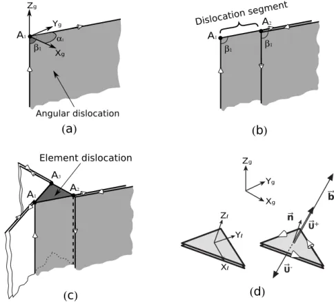
Angular, biangular and triangular dislocations

Among the different ways to build a triangular element with angular dislocations, the simplest (Fig. 1.3) is created by superposition of three angular dislocations as described by Yoffe (Yoffe, 1960). All three angular dislocations lie in the same plane, here the (x, y) − plane, and the dislocation surfaces (lightly shaded areas) extend to infinity. This construction does not enable a solution for the half-space problem as the lines of some dislocations would cross the traction-free surface when the element is inclined. Conse-quently, Comninou (Comninou and Dundurs,1975) did not adopt this simple representa-tion in their solurepresenta-tion for the angular dislocarepresenta-tion in the half-space. Instead, they used an angular dislocation with one vertical leg perpendicular to the surface of the half-space. An angular dislocation (A, α, β) (Fig. 1.4a) lies in a vertical plane that makes an angle

Figure 1.3: _{Triangular element construction according to Yoffe (Yoffe, 1960). All} three angular dislocations lie in the same plane. This construction does not enable a solution for the half-space problem as the lines of some dislocations may cross the

traction-free surface when the element is inclined

Figure 1.4: _{Angular, biangular, triangular dislocations and local coordinate system} used in iBem3D. (a) Angular dislocation representation, with its semi-infinite vertical and inclined legs initiating at point A. (b) Biangular dislocation construction from two angular dislocations. The inclined leg cancels at point B. (c) Triangular dislocation construction from three biangular or six angular dislocations. All inclined and vertical legs cancel, leaving a triangular loop represented by the element, where a constant Burgers’s vector is applied. (d) Representation of the element local coordinate system

and the Burgers vector

β in the horizontal plane to the global y − axis, with one leg perpendicular to the free surface. The two legs of the angular dislocation subtend an angle α, and extend to infinity from a common vertex A. The uniform displacement discontinuity across the dislocation is given by its Burgers vector. Given a point M in the elastic body, the displacement

component ˚ui due to an angular dislocation (A, α, β) (Fig. 1.4a), is given by: ˚ui(M) = 3 X j=1 ˚ Uij(M, A, α, β)bj = ˚Uijbj (Einstein notation) (1.1)

and is a linear function of the Burgers vector b. Coefficients of the matrix ˚Uij, called

the displacement influence matrix, are given by Comninou & Dundurs (Comninou and

Dundurs,1975). Note that the half-space problem is solved using image dislocations and

a solution to the Boussinesq problem to remove tractions from the free surface (Comninou

and Dundurs, 1975). The Boussinesq solution provides corrective terms for the free

sur-face so that no shear stresses appear on it, and the image dislocations remove the normal tractions.

The strain field at point M can be computed by partial derivation of (1.1) by using the linearized Green-St Venant strain tensor:

˚ǫij= 1 2(∇˚u + ∇˚u t_{) =} 3 X k=1 ˚_{Eijk(M, A, α, β)bk= ˚Eijkbk (1.2)} where ∇˚u is the deformation gradient tensor. ˚Eijk represents the strain influence matrix

due to an angular dislocation and is derived from: ˚_{Eijk =} 1 2 ∂˚Uik ∂xj + ∂˚Ujk ∂xi ! (1.3) For linear elastic materials, the stress components are related to the infinitesimal strain components using constitutive equations called Hooke’s Law. The general form of Hooke’s Law is simplified for an isotropic material, so there are only two material constants. The isotropic elastic material is one in which the elastic constants are the same regardless of direction. Given the Hooke’s law

σij = 2Gǫij + λǫkkδij (1.4)

the stress tensor is given for infinitesimal deformation as ˚σij= 2G˚ǫij+ λ˚ǫkkδij= 3 X k=1 ˚_{Sijk(M, A, α, β)bk} = ˚Sijkbk (1.5)

where G is the shear modulus, λ the Lam´e’s constant, δij the Kronecker delta, and ˚ǫij is

given by (1.2). ˚Sijk represents the stress influence matrix due to an angular dislocation.

A biangular dislocation, having two vertical legs, perpendicular to the free surface, con-structed from two angular dislocations (A0, α, β) and (A1, α, β) (Fig. 1.4b). The resulting

displacement at point M is simply the superposition of contributions from the two angular dislocations: ¯ ui(M) = 3 X j=1 [˚Uij(M, A0, α, β) − ˚Uij(M, A1, α, β)]bj = 3 X j=1 ¯ Uij(M, A0, A1, α, β)bj = ¯Uijbj (1.6)

Using the same process of superposition, a triangular element {A0, A1, A2} in the

whole-or half-space is build with three biangular dislocations (Fig. 1.4c). The superposition of these dislocations are vertical surfaces defining a volume. This volume is semi-infinite and vertically trending compared to the global coordinate system. The coincident legs under each vertex cancel leaving a displacement discontinuity only in the triangle. The Burgers vector b is constant over the triangular dislocation. The superposition of these dislocations are vertical surfaces defining a volume. This volume is semi-infinite and vertically trending compared to the global coordinate system.

The total displacement at point M resulting from a triangular dislocation made of three dislocation segments, is therefore given by

ui(M) = 3 X j=1 3 X k=1 ¯ Uij(M, Ak, Ak+1, αk, βk)bj = Uijbj (1.7) the strain by ǫij(M) = 3 X k=1 3 X l=1 ¯ Eijk(M, Al, Al+1, αl, βl)bk = Eijkbk (1.8)

and the stress by

σij(M) = 3 X k=1 3 X l=1 ¯ Sijk(M, Al, Al+1, αl, βl)bk= Sijkbk (1.9)

For a model made of n triangular dislocation elements, the displacement at any point M is determined by superposition, i.e. by contribution of all the elements within the elastic body: ui(M) = n X m=1 Umijb m j = U m ijb m j (1.10) where Um

ij are the displacement influence coefficients due to the mth element, and bmj is

the jth_{Burgers vector component. The strain and stress also are given by the contribution}

of all elements.

The Burgers vector b, for a given element e, can be divided into two displacement vectors, u+ _{on the positive side of the element and u}− _{on the negative side, and these are related}

by:

b = u+_{− u}− (1.11) In order to retrieve these vectors, one first calculates the displacement u+_{at the element’s}

centroid using equation (1.10) with an infinitesimal positive shift along the element’s nor-mal as described in section 1.9.2.2 of the appendix. The displacement on the negative side, u−_{, is then calculated using the prescribed boundary value and (1.11).}

Note that one must use the corrective displacement presented in appendix if the observa-tion point M is under the triangulated surfaces of discontinuity in the elastic half-space, since the displacement field is not correctly calculated. This problem is directly linked to the construction of the triangular element and the interpretation of the solid angle used to define Burgers’function (see appendix).

1.4.2

Element boundary conditions

Each triangular dislocation is defined with three boundary conditions using the element local coordinate system. This is constructed with x along the dip (direction of greatest inclination in the element plane), z along the element’s normal, and y is the cross-product of z and x. The y-axis is oriented toward north if the element is horizontal with respect to the global coordinate system (Fig. 1.4d). Boundary conditions consist of the displace-ment discontinuity component or traction component in each coordinate direction. When all triangular dislocations within the model are prescribed with displacement discontinu-ities, the displacement at any point within the elastic field is entirely defined by equation (1.10). However, when triangular elements have prescribed traction boundary condition,

one must first determine the corresponding Burgers components that produce these trac-tions, and then proceed with (1.10).

Using Cauchy’s formula by resolving the stress tensor σij (Eq. 1.9) on the triangular

element’s plane using its centroid as the collocation point, the element’s traction can now be defined by:

ti = σijnj = (Sijkbk) nj = (Sijknj) bk= Tijbk (1.12)

where nj represents the element’s normal components and Tij = Sijknj is the traction

influence matrix.

Using the traction formulation for a triangular dislocation, the total traction at the center of a triangular element is simply the total traction exclusive of that imposed by the remote loading at the center:

ti = Tmijb m

j (1.13)

A system of linear equations is then constructed using (1.13), and solved for the unknowns Burgers vector components

{t} = [T]{b} (1.14) In equation (1.14_{), {t} represents the column of the initially prescribed traction vectors}

(see next section 1.4.3_{), [T] is a dense matrix of traction influence coefficients, and {b}}

the column of the unknowns Burgers vectors.

1.4.3

Remote loading

Initial boundary conditions are prescribed for each triangular element of the model based upon the stress field σR _{that exists throughout the body before any slip or opening of the}

elements. This remote stress is applied to the model by prescribing boundary conditions that are the tractions resolved from this remote stress on the elements using Cauchy’s formula (1.12). Then, one uses equation (1.14) to solve the system. Given the far field remote stress σR _{and the normal n of an element e, the initial traction for this element is}

given by t = −σR_{n. Therefore, the initial traction boundary vector for a given element}

opposes the prescribed resolved far field stress onto this element, leading to equilibrium. If a remote strain ǫR_{is prescribed, one first calculates the corresponding remote stress σ}R

1.4.4

Post-processing at observation points

After the system (1.14) is solved, displacement, strain and stress components can be computed anywhere within the elastic solid, by using the principle of superposition. For a given observation point (field point), the resulting component is the sum of contributions from all influencing elements (sources). For the displacement, equation (1.10) is used directly. For strain and stress, equation (1.15) and (1.16) are used respectively:

ǫij(M) = n X m=1 Em ijkb m k + ǫ R ij = E m ijkb m k + ǫ R ij (1.15) σij(M) = n X m=1 Smijkb m k + σ R ij = S m ijkb m k + σ R ij (1.16) where Em

ijk and Smijk represent the strain and stress influence matrices at field point M

due to a source element m, respectively, and ǫR _{and σ}R _{the remote field strain and stress,}

respectively. In equation (1.15) and (1.16), the perturbed strain/stress field due to slipping triangular elements is simply superimposed on the remote stress/strain field.

1.4.5

Benchmarking the code

The basic element used by iBem3D is a planar dislocation loop with a triangular tipline. The analytical equations for the displacement, strain, or stress fields around such an element are not written down because the element is actually made up of a set of angular dislocations and the effect of these are numerically summed within the code. Therefore we must use a simpler dislocation solution for the purpose of benchmarking the code and find a way to compare that to the output of iBem3D. Figure1.5shows a single dislocation line extending along the z coordinate axis with a tangent vector in the positive coordinate direction. The edge dislocation is positive with a Burgers vector directed along the x coordinate axis. For comparison to this dislocation line we choose the simplest iBem3D element, an equilateral triangular element with unit side length, a = 1. This element lies in the (x, z)-plane with one side parallel to the z coordinate axis. The tangent vector along that side points in the positive coordinate direction and the dislocation there is a pure edge dislocation with Burgers vector directed along the x coordinate axis. The origin of coordinates is placed at the midpoint of that side. Because the dislocation line is infinite in length and the side of the triangular element is finite, we must restrict our range to the region immediately surrounding the side of the element at the midpoint.