Volcanic SO₂ fluxes derived from satellite data: a survey using OMI, GOME-2, IASI and MODIS

HAL Id: hal-00768974

https://hal.archives-ouvertes.fr/hal-00768974

Submitted on 20 Oct 2015

HAL is a multi-disciplinary open access

archive for the deposit and dissemination of

sci-entific research documents, whether they are

pub-lished or not. The documents may come from

teaching and research institutions in France or

abroad, or from public or private research centers.

L’archive ouverte pluridisciplinaire HAL, est

destinée au dépôt et à la diffusion de documents

scientifiques de niveau recherche, publiés ou non,

émanant des établissements d’enseignement et de

recherche français ou étrangers, des laboratoires

publics ou privés.

using OMI, GOME-2, IASI and MODIS

Nicolas Theys, Robin Campion, Lieven Clarisse, Hugues Brenot, J. van Gent,

Bart Dils, S. Corradini, L. Merucci, Pierre-François Coheur, Michel van

Roozendael, et al.

To cite this version:

Nicolas Theys, Robin Campion, Lieven Clarisse, Hugues Brenot, J. van Gent, et al.. Volcanic SO2

fluxes derived from satellite data: a survey using OMI, GOME-2, IASI and MODIS. Atmospheric

Chemistry and Physics, European Geosciences Union, 2013, 13 (12), pp.5945-5968.

�10.5194/acp-13-5945-2013�. �hal-00768974�

Atmos. Chem. Phys., 13, 5945–5968, 2013 www.atmos-chem-phys.net/13/5945/2013/ doi:10.5194/acp-13-5945-2013

© Author(s) 2013. CC Attribution 3.0 License.

EGU Journal Logos (RGB)

Advances in

Geosciences

Open Access

Natural Hazards

and Earth System

Sciences

Annales

Geophysicae

Nonlinear Processes

in Geophysics

Atmospheric

Chemistry

and Physics

Atmospheric

Chemistry

and Physics

Atmospheric

Measurement

Techniques

Atmospheric

Measurement

Techniques

Biogeosciences

Open Access Open Access

Biogeosciences

Discussions

Climate

of the Past

Open Access Open Access

Climate

of the Past

Discussions

Earth System

Dynamics

Open Access Open Access

Earth System

Dynamics

Geoscientific

Instrumentation

Methods and

Data Systems

Open Access

_{Geoscientific}

Instrumentation

Methods and

Data Systems

Geoscientific

Model Development

Open Access Open Access

Geoscientific

Model Development

Hydrology and

Earth System

Sciences

Hydrology and

Earth System

Sciences

Ocean Science

Open Access Open Access

Ocean Science

Discussions

Solid Earth

Open Access Open Access

Solid Earth

Discussions

The Cryosphere

Open Access Open Access

The Cryosphere

Natural Hazards

and Earth System

Sciences

Open Access

Discussions

Volcanic SO

2

fluxes derived from satellite data: a survey using OMI,

GOME-2, IASI and MODIS

N. Theys1, R. Campion2,*, L. Clarisse2, H. Brenot1, J. van Gent1, B. Dils1, S. Corradini3, L. Merucci3, P.-F. Coheur2, M. Van Roozendael1, D. Hurtmans2, C. Clerbaux4,2, S. Tait5, and F. Ferrucci5

1_{Belgian Institute for Space Aeronomy (BIRA-IASB), Brussels, Belgium}

2_{Spectroscopie de l’Atmosph`ere, Service de Chimie Quantique et Photophysique, Universit´e Libre de Bruxelles (ULB),} Brussels, Belgium

3_{Istituto Nazionale di Geofisica e Vulcanologia (INGV), Rome, Italy}

4_{UPMC Univ. Paris 6, Universit´e Versailles St.-Quentin, CNRS/INSU, LATMOS-IPSL, Paris, France} 5_{Institut de Physique du Globe de Paris (IPGP), Paris, France}

*_{now at: Instituto de Geofisica, Universidad Nacional Aut´onoma de Mexico, Mexico City, Mexico}

Correspondence to: N. Theys (theys@aeronomie.be)

Received: 18 September 2012 – Published in Atmos. Chem. Phys. Discuss.: 6 December 2012 Revised: 18 May 2013 – Accepted: 21 May 2013 – Published: 20 June 2013

Abstract. Sulphur dioxide (SO2)fluxes of active degassing volcanoes are routinely measured with ground-based equip-ment to characterize and monitor volcanic activity. SO2 of unmonitored volcanoes or from explosive volcanic eruptions, can be measured with satellites. However, remote-sensing methods based on absorption spectroscopy generally provide integrated amounts of already dispersed plumes of SO2and satellite derived flux estimates are rarely reported.

Here we review a number of different techniques to de-rive volcanic SO2 fluxes using satellite measurements of plumes of SO2 and investigate the temporal evolution of the total emissions of SO2for three very different volcanic events in 2011: Puyehue-Cord´on Caulle (Chile), Nyamula-gira (DR Congo) and Nabro (Eritrea). High spectral resolu-tion satellite instruments operating both in the ultraviolet-visible (OMI/Aura and GOME-2/MetOp-A) and thermal infrared (IASI/MetOp-A) spectral ranges, and multispec-tral satellite instruments operating in the thermal infrared (MODIS/Terra-Aqua) are used. We show that satellite data can provide fluxes with a sampling of a day or less (few hours in the best case). Generally the flux results from the different methods are consistent, and we discuss the advantages and weaknesses of each technique. Although the primary objec-tive of this study is the calculation of SO2fluxes, it also en-ables us to assess the consistency of the SO2products from the different sensors used.

1 Introduction

1.1 Importance of SO2fluxes in volcano monitoring Volcanism is the surface expression of internal processes, driven by heat generated in the Earth’s interior. During erup-tions, solid, liquid and gaseous products are generated. The main driving force behind eruptions is exsolution of gas from magma during decompression, which drives ascent through the Earth’s crust. Sulfur dioxide (SO2) is one of the most abundant compounds among volcanic gases (e.g., Le Guern et al., 1982; Symonds et al., 1994; and Oppenheimer et al., 2011, among others). Since this gas is very soluble in wa-ter and is thermodynamically unstable at low temperature, the presence of SO2 in volcanic plumes is characteristic of a high emission temperature. SO2plumes are the markers of volcanic activity that may be classified into two main types.

– Explosive activity: rapid exsolution of volcanic gases in the volcanic conduit generates an ensemble of par-ticles (tephra) through fragmentation that is ejected ex-plosively into the atmosphere forming a plume. Heat is derived from the erupted tephra and emitted gases, and atmospheric air is entrained, which increases buoyancy. Additional latent heat may be released as water con-denses and freezes in the plume. Volcanic plume heights may reach altitudes well into the stratosphere and the

maximum height depends on the mass flux rate (amount of material released as a function of time), the size dis-tribution of erupted particles, and the local wind field. – Effusive activity: driven by gas exsolution, although at

lower rates than during magma fragmentation, molten rock products (lava flows) are erupted at the surface. This style of activity also results in particle generation but the “particles” (magma clots, vesicular scoria) are usually coarse enough to fall out close to the vent. Mag-matic gases released are hot and may still produce a sig-nificant plume. Thermal energy is also available from the lava, however, these plumes tend only to reach mid-tropospheric levels except in some exceptional cases. The main conclusion from the above is that the height at which magmatic gases are injected is not arbitrary but strongly dependent on the eruption regime. As we will show, the height at which SO2is present in the atmosphere also has a large influence on the techniques for detecting the amounts present, hence the height becomes a central issue for the char-acterization of plumes.

The most useful quantity for volcano monitoring is gen-erally the SO2 flux (expressed in kg s−1 or kT day−1), which, combined with other monitoring and petrographic data, yields unique insights into the dynamics of degassing magma. Changes in SO2 flux are often used as an eruption precursor (e.g., Olmos et al., 2007; Inguaggiato et al., 2011; and Werner et al., 2011). The SO2flux is a marker of impor-tant volcanic processes as, in particular: (1) replenishment of the magmatic system with juvenile magma (e.g., Caltabiano et al., 1994; and Daag et al., 1996), characterized by a grad-ual increase of the measured SO2flux over a relatively long time period, (2) volatile exhaustion of a degassing or erupt-ing magma body. These processes are marked by a gradual decrease in the SO2flux (e.g., Kazahaya et al., 2004) and, as the gases are the driving force of volcanic eruptions, gener-ally precede the end of an eruptive period, and (3) plugging of the upper conduit system by crystallizing magma (e.g., Fischer et al., 1994). This process promotes gas accumula-tion under the plug, until its destrucaccumula-tion or failure when its resistance is exceeded, which is believed to fuel long last-ing “vulcanian” and “strombolian” activity (e.g., Iguchi et al., 2008). However, in certain circumstances, SO2 measure-ments are less useful. This is the case when dissolution of the gas occurs in a hydrothermal system located between the magma and the surface (Symonds et al., 2001). This process, also known as scrubbing, can complicate the interpretation of SO2flux data, being not related to real magmatic processes. An overview on degassing from volcanoes can be found in Shinohara (2008) and Oppenheimer et al. (2011).

Measuring time series of SO2 flux and integrating them over time is also crucially important for the quantification of the volcanic contribution to the global sulfur budget in the Earth system. SO2 is, as a precursor of sulfate aerosols, important for air quality (Chin and Jacob, 1996) and climate

(Haywood and Boucher, 2000; Rampino et al., 1988). Strato-spheric injection of SO2especially can have a dramatic im-pact on the global climate (Robock, 2000; Solomon et al., 2011; Bourassa et al., 2012). SO2fluxes are also key for es-tablishing a total gas emission inventory of volcanoes. In-deed, emission fluxes of all the other volcanogenic com-pounds into the atmosphere are usually calculated by scal-ing their concentration ratio [X]/[SO2] to the SO2flux (e.g., Aiuppa et al., 2008). This inventory is important in volcano monitoring (e.g., CO2at Stromboli, and Aiuppa et al., 2011), for studying the volcanic impact on the local atmospheric chemistry (e.g., Oppenheimer et al., 2010) and on the en-vironment (Delmelle et al., 2002), or for quantifying green-house gas emissions from volcanoes.

1.2 Measurements of volcanic SO2fluxes

Remote measurements of magmatic volatiles have focused a lot on SO2because it is arguably the most readily measurable by absorption spectroscopy, due to its low background con-centration in the atmosphere (∼ 1 ppbv in clean air; Breeding et al., 1973), and the strong and distinctive structures in its absorption spectrum both at ultraviolet (UV) and thermal in-frared (TIR) wavelengths (see the HITRAN database; Roth-man et al., 2009). Measurements of volcanic SO2fluxes are widely carried out from the surface since the mid-seventies using the Correlation Spectrometer (COSPEC) instrument (Stoiber et al., 1983; Stix et al., 2008). More recently, con-solidated measurements of total emission fluxes of SO2have also been made possible for a network of active degassing volcanoes (Network for Observations of Volcanic and At-mospheric Change – NOVAC; Galle et al., 2010 and ref-erences therein), with the advent of inexpensive and high-quality scanning miniaturized differential optical absorption spectroscopy instruments (Mini-DOAS).

For unmonitored volcanoes or explosive volcanic erup-tions, space-based measurements of SO2 are more appro-priate. Since 1978, the Total Ozone Mapping Spectrome-ter (TOMS) and follow-up instruments have been measuring SO2in the UV spectral range (Krueger, 1983; Krueger et al., 1995), although with a rather high detection limit, and helped to establish the long-term volcanic input of SO2 into the high atmosphere (Carn et al., 2003a; Halmer et al., 2002). In the infrared, space-based sounding of SO2was also possible with TOVS (Prata et al., 2003), with data going back to 1978. Over the last two decades, SO2measurements from space-based nadir sensors have undergone an appreciable evolu-tion, owing to improved spectral resoluevolu-tion, coverage and spatial resolution (Thomas and Watson, 2010). The follow-ing instruments have been used with measurement channels that correspond to the infrared and ultraviolet SO2absorption bands: GOME (Eisinger and Burrows, 1998), SCIAMACHY (Afe et al., 2004), OMI (Krotkov et al., 2006), GOME-2 (Rix et al., 2009, 2012), MODIS (Watson et al., 2004; Corradini et al., 2009), ASTER (Urai, 2004; Campion et al., 2010),

SEVIRI (Prata and Kerkman, 2007; Corradini et al., 2009), AIRS (Prata and Bernardo, 2007) and IASI (Clarisse et al., 2008, 2012; Walker et al., 2012; Carboni et al., 2012). Com-pared to ground-based measurements, daily satellite mea-surements provide a comprehensive cartography of volcanic emissions at a global scale, but only the strongest sources are picked up due to the limitations in the ground resolution and/or sensitivity of the current sensors.

The standard output of satellite SO2 retrievals is not a flux but a vertical column (VC). It represents the amount of SO2 molecules in a column overhead per unit surface area (generally expressed in Dobson unit – 1 DU: 2.69 × 1016 molecules cm−2). From the SO2 VCs, one can easily cal-culate the total SO2 mass (knowing the satellite pixel size), which is a quantity useful to investigate volcanic activity. For example, Carn et al. (2008) monitored degassing of vol-canoes in Ecuador and Colombia and showed that the cor-responding SO2 masses had some correlation with volcano seismicity and local observation of volcanic activity.

Estimating fluxes from emitted masses is notoriously dif-ficult and implies more than applying (crude) scaling laws to the measured total SO2 masses. Until now, there have been only a handful of studies addressing the problem of SO2 flux estimates from space (Carn and Bluth, 2003; Urai, 2004; Pugnaghi et al., 2006; Campion et al., 2010; Merucci et al., 2011; Boichu et al., 2013; Carn et al., 2013). One difficulty comes from the fact that accurate flux calculations require additional information (not always well characterized) on the transport and loss of SO2following its release into the atmo-sphere. Another important issue arises from the limitations in terms of accuracy of the SO2VCs retrieved and subsequently used. Indeed, satellite SO2retrievals are not always in good agreement (see e.g., Prata, 2011). This is believed to be due to, for example, the impact of the calculated or assumed SO2 plume height on the retrievals or to different sensitivities of the UV and IR bands to SO2, aerosols and clouds. Note that, in spite of its general interest from a remote-sensing point of view and for the calculations of SO2fluxes, a comprehen-sive intercomparison and validation study has hitherto not yet been carried out.

For all these reasons, strong and long-lasting volcanic eruptions are challenging as they produce a vertically dis-tributed SO2 mass profile, which is highly variable in time in response to the instantaneous eruptive power. Once emit-ted, SO2is dispersed along different transport pathways de-pending on injection altitude due to the vertical shear of the horizontal wind. Consequently, the SO2plume may be very inhomogeneous in space. Moreover, the SO2plume may ex-tend over long distances (> 1000 km) and is then often only partly covered by satellite instruments that do not provide full daily global coverage. An additional difficulty comes from the fact that a multi-layered SO2plume is probed by a given satellite instrument with a measurement sensitivity strongly dependent on the altitude. Furthermore, if SO2is distributed

in different altitude layers, each of them is characterized by different SO2loss rates.

The motivation for this collaborative study is an effort to estimate volcanic SO2 fluxes using satellite measure-ments of plumes of SO2. We make use of the SO2 prod-ucts from the high spectral resolution OMI, GOME-2 (UV), IASI (TIR) and multispectral resolution MODIS (TIR) in-struments. These are currently used in an automated mode to provide alerts for aviation safety (as a proxy for the pres-ence of volcanic ash) or for volcano monitoring, in the Sup-port to Aviation Control Service (SACS; Brenot et al., 2013), the European Volcano Observatory Space Services (EVOSS; Ferrucci et al., 2013) and the Support to Aviation for Vol-canic Ash Avoidance (SAVAA; Prata et al., 2008) projects. We combine and compare four different approaches and in-vestigate the time evolution of the total emissions of SO2for three volcanic events (different in type) occurring in 2011: Puyehue-Cord´on Caulle, Chile (using IASI), Nyamulagira, DR Congo (using OMI and GOME-2) and Nabro, Eritrea (using IASI, GOME-2 and MODIS).

Although the main objective of this study is the determina-tion of SO2fluxes, we also investigate the consistency of the SO2products from the different sensors used. Results from the OMI and GOME-2 UV instruments (with similar vertical measurement sensitivities) are compared, as the calculation of fluxes is in principle not affected by spatial resolution is-sues. Furthermore, SO2masses results from GOME-2, IASI – both on MetOp-A – and MODIS are compared for con-ditions where additional information on the altitude of the plume is available.

In the next section we give an overview of the instru-ments and algorithms used to retrieve SO2vertical columns. In Sect. 3 we describe the methods to derive SO2fluxes. Re-sults are presented in Sect. 4 and conclusions are given in Sect. 5.

2 Satellite SO2data 2.1 GOME-2

The second Global Ozone Monitoring Experiment (GOME-2) is a UV/visible spectrometer covering the 240–790 nm wavelength interval with a spectral resolution of 0.2–0.5 nm (Munro et al., 2006). GOME-2 measures the solar radiation backscattered by the atmosphere and reflected from the sur-face of the Earth in a nadir viewing geometry. A solar spec-trum is also measured via a diffuser plate once per day. The GOME-2 instrument is in a sun-synchronous polar orbit on board the Meteorological Operational satellite-A (MetOp-A), launched in October 2006, and has an Equator crossing time of 09:30 LT (local time) on the descending node. The ground pixel size is nearly constant along the orbit and is 80 km ×40 km. The full width of a GOME-2 scanning swath is 1920 km, allowing nearly global coverage every day. In

addition to its nominal swath width, GOME-2 performs once every four weeks measurements in a narrow swath mode of 320 km with increased spatial resolution.

The spectral range and resolution of GOME-2 allows the retrieval of a number of absorbing trace gases such as O3, NO2, SO2, H2CO, CHOCHO, OClO, H2O, BrO, as well as cloud and aerosol parameters. The SO2vertical columns are routinely retrieved from GOME-2 UV backscatter mea-surements of sunlight (Rix et al., 2009, 2012; van Geffen et al., 2008) using the Differential Optical Absorption Spec-troscopy (DOAS) technique (Platt and Stutz, 2008). In a first step, the columnar concentration of SO2along the effective light path through the atmosphere (the so-called slant col-umn) is determined using a nonlinear spectral fit procedure. Absorption cross sections of atmospheric gases (SO2, O3and NO2)are adjusted to the log ratio of a measured calibrated earthshine spectrum and a solar (absorption free) spectrum in the wavelength interval from 315 to 326 nm. Further correc-tions are applied to account for Rayleigh and rotational Ra-man scattering and various instrumental spectral features. In a second step, a background correction is applied to the data to avoid nonzero columns over regions known to have very low SO2and to ensure a geophysical consistency of the re-sults at high solar zenith angles (where a strong interference of the SO2and ozone absorption signals lead to negative SO2 slant columns). In a third step, the SO2slant column is con-verted into a vertical column using a conversion factor (called air mass factor), estimated from simulations of the transfer of the radiation in the atmosphere. It accounts for parame-ters influencing photon paths: solar zenith angle, instrument viewing angles, surface albedo, atmospheric absorption, scat-tering on molecules, and clouds. For the air mass factor cal-culation, a SO2concentration vertical profile is also required. As the information on the SO2plume height is generally not available at the time of observation, three vertical columns are computed for different hypothetical SO2plume heights: 2.5, 6 and 15 km above ground level (see Sect. 2.5). It should also be noted that an important error source exists for high SO2column amount (> 50–100 DU), when the SO2 absorp-tion tends to saturate leading to a general underestimaabsorp-tion of the SO2columns.

2.2 OMI

The Ozone Monitoring Instrument (OMI) is a Dutch/Finnish instrument flying on the AURA satellite of NASA (launched in July 2004) on a sun-synchronous polar orbit with a period of 100 min and an Equator crossing time of about 13:45 LT on the ascending node. OMI is a nadir-viewing imaging spec-trograph that measures atmosphere-backscattered sunlight in the ultraviolet-visible range from 270 to 500 nm with a spec-tral resolution of about 0.5 nm (Levelt et al., 2006). In con-trast to GOME-2, operating with a scanning mirror and one-dimensional photo diode array detectors, OMI is equipped with two-dimensional CCD (charge-coupled device)

detec-tors, recording the complete 270–500 nm spectrum in one di-rection, and observing the Earth’s atmosphere with a 114◦ field of view, distributed over 60 discrete viewing angles, perpendicular to the flight direction. The field of view of OMI corresponds to a 2600 km wide spatial swath. In this way complete global coverage is achieved within one day. Depending on the position across the track, the size of an OMI pixel varies from 13 km ×24 km at nadir to 13 km ×128 km for the extreme viewing angles at the edges of the swath. It should be stressed that due to a blockage affect-ing the nadir viewaffect-ing port of the sensor, the radiance data of OMI are altered at all wavelengths for some particular view-ing directions of OMI. This row anomaly (changview-ing over time) can affect the quality of the products and hence reduce the spatial coverage of the data (see http://www.knmi.nl/ omi/research/product/rowanomaly-background.php). In this study, the OMI row anomaly pixels have been filtered by us-ing the quality flag (QualityFlag PBL, Bit 11) in the OMSO2 L2 files.

From solar back-scattered measured radiances, SO2 ver-tical columns are retrieved using the linear fit algorithm (Yang et al., 2007). The technique uses OMI measurements at several discrete UV wavelengths to yield total SO2 and ozone columns as well as effective reflectivity (see also http://so2.gsfc.nasa.gov and http://satepsanone.nesdis.noaa. gov/pub/OMI/OMISO2/index.html). Radiative transfer cal-culations account for the observation geometry, Rayleigh and Raman scattering, atmospheric absorption, surface albedo, aerosols and clouds. Similarly to GOME-2 retrieval, the OMI SO2columns are provided for a set of layers with assumed center of mass heights at 0.9, 2.5, 7.5 and 17 km.

2.3 IASI

The hyperspectral Infrared Atmospheric Sounding Interfer-ometer (IASI) was launched in 2006 onboard MetOp-A (Clerbaux et al., 2009; Hilton et al., 2012) for meteorological and scientific applications. Global nadir measurements are acquired twice a day (at 09:30 and 21:30 mean local equa-torial time) with a small to medium sized footprint (from a 12 km diameter circle at nadir to an ellipse with 20 and 39 km axes at its largest swath). The instrumental characteristics of IASI are state-of-the-art with an uninterrupted spectral cov-erage from 645 to 2760 cm−1, apodized spectral resolution of 0.5 cm−1and instrumental noise mostly below 0.2 K below 2000 cm−1.

Operational products of IASI distributed by EUMETSAT include temperature and humidity profiles, surface and cloud parameters and selected trace gases. IASI measurements can be used to retrieve a host of trace gases (Clarisse et al., 2011). Some on global daily scale (e.g., CO2, H2O, CO, O3, HCOOH, CH3OH, NH3, and CH4), others on a more spo-radic basis (e.g., HONO, C2H4, SO2, and H2S).

The spectral range from IASI covers three SO2absorption bands, the ν1band in the ∼ 8.5 µm atmospheric window; the

strong ν3band at ∼ 7.3 µm and the combination band ν1+ν3 at ∼ 4 µm. In this study, we make use of the SO2 columns generated by the algorithm presented in Clarisse et al. (2012). The retrieval combines measured brightness temperature dif-ferences between baseline channels and channels in the SO2 absorption ν3band (at 1371.75 cm−1and 1385 cm−1). The vertical sensitivity to SO2is affected by water vapor absorp-tion and is limited to the atmospheric layers above 3–5 km height. The conversion of the measured signal into a SO2 ver-tical column is performed by making use of a large look-up-table and EUMETSAT operational pressure, temperature and humidity profiles. The algorithm calculates the SO2columns for a set of pre-defined hypothetical altitude levels: 5, 7, 10, 13, 16, 19, 25 and 30 km. The main features of the algorithm are a wide applicable total column range (over 4 orders of magnitude, from 0.5 to 5000 DU), low noise level and a low theoretical uncertainty (3–5 %).

2.4 MODIS

The Moderate Resolution Imaging Spectroradiometer (MODIS) is a multispectral instrument on board the NASA-Terra and NASA-Aqua polar satellites (Barnes et al., 1998, http://modis.gsfc.nasa.gov). Terra’s descending node (from north to south) crosses the Equator in the morning at about 10:30 LT, while the Aqua ascending node (south to north) crosses the Equator at about 13:30 LT. MODIS acquires data in 36 spectral bands from visible to thermal infrared and its spatial resolution varies between 250, 500 and 1000 m. The sensor scans ±55◦across-track resulting in a 2330 km swath and full global coverage every one to two days.

As IASI, MODIS covers all the three infrared SO2 absorp-tion bands, ν1, ν3and ν1+ν3. The ν1+ν3absorption feature (channel 23) lies in a transparent window but is very weak and affected by scattered solar radiation during the day. The strongest ν3signature (channel 28) is highly affected by the atmospheric water vapor absorption so that the SO2retrieval is accurate only for plumes in the middle troposphere/lower stratosphere. Finally the ν1feature (channel 29) lies in a rel-atively transparent spectral region and can be used to re-trieve also the lower tropospheric SO2. The latter is, how-ever, highly affected by the volcanic ash absorption and the retrieval is very sensitive to uncertainties on surface temper-ature and emissivity (Corradini et al., 2009; Kearney et al., 2009).

The SO2retrieval scheme for multispectral TIR measure-ments was first described by Realmuto et al. (1994) for the TIMS airborne spectrometer and was based on a weighted least squares fit procedure using instrumental measured radi-ances and simulated radiradi-ances obtained by varying the SO2 amount. Further work carried out by several authors allowed the extension of SO2 retrieval to different satellite sensors such as MODIS (Watson et al., 2004), ASTER (Realmuto et al., 1997; Pugnaghi et al., 2006) and SEVIRI (Corradini et al., 2009). Here we refer to the procedure scheme described

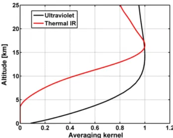
Fig. 1. Averaging kernels for satellite retrievals of SO2at ultravio-let and thermal infrared wavelengths for a typical clear-sky tropical atmosphere.

by Corradini et al. (2009) in which the SO2column amount is retrieved on a pixel by pixel basis using the ν3 signature and top of the atmosphere (TOA) simulated radiances.

The TOA radiances look up tables are obtained from MODTRAN 4 computations driven by the atmospheric pro-files (pressure, temperature and humidity), the plume ge-ometry (plume altitude and thickness) and varying the SO2 amounts. The volcanic cloud top height has been determined assuming the cloud top temperature of the opaque parts of the cloud to be equal to the ambient temperature and deriving the height from the temperature vertical profile (Prata and Grant, 2001; Corradini et al., 2010).

2.5 Altitude-dependent sensitivity

One of the largest errors on the SO2columns is due to a poor a priori knowledge of the height of the SO2plumes. To as-sess this effect on the retrievals presented above, it is useful to consider the satellite SO2column averaging kernels. The averaging kernel is defined as the derivative of the retrieved vertical column with respect to the partial column profile (Ja-cobian), and basically reflects the changes in measurement sensitivity along the vertical axis. As an illustration, Fig. 1 shows examples of functions for UV (GOME-2 and OMI retrievals) and thermal IR (IASI and MODIS ν3retrievals) wavelengths.

The UV averaging kernel in Fig. 1 shows the typical be-havior of the satellite measurement sensitivity to SO2located at different altitudes, with almost constant values in the up-per troposphere and lower stratosphere and then a decrease below ∼ 10 km, essentially due to increasing Rayleigh scat-tering in the troposphere. One can see that SO2located at the surface will produce a signal an order of magnitude lower than if it was in the stratosphere. For the TIR measurement,

the effect of altitude on the measurement sensitivity is mod-est in the stratosphere but is critical in the troposphere be-cause of the sharp temperature gradient. The maximum value is reached at the tropopause (∼ 16 km), where the thermal contrast between the plume and the background radiation is highest. Below 5 km altitude, almost no sensitivity to SO2is observed because of strong water vapor absorption.

It should be emphasized that no conclusions can be drawn from Fig. 1 on the SO2detection limit as the averaging ker-nel calculations are independent of the signal-to-noise ratios (specific to each instrument).

3 Methods to derive SO2fluxes

As evocated previously, turning from SO2VCs or masses to flux data is nontrivial. In this section, we review several ex-isting methods; a summary of which can be found in Table 1 (Sect. 5).

All the techniques are based on mass conservation in that a satellite SO2image obtained on a given day reflects the bud-get of SO2 emissions and losses (through oxidation and/or deposition) since the start of the eruption. Hence, the re-trieval of SO2 fluxes from a sequence of consecutive SO2 images generally requires a sufficiently good estimate of the loss term, although in some instances the loss of SO2may be considered negligible (e.g., close to the volcano; McGonigle et al., 2004). The simplifying assumption we made through-out this work and which is also supported by literature (re-view in Eatough et al., 1994), is that the kinetics of the SO2 removal follow a first order law:

∂c

∂t = −k · c, (1)

where c is the SO2concentration and k is the reaction rate constant (s−1), which is also often expressed as k = 1/τ , where τ is the SO2e-folding time. A difficulty of using this assumption is that k is extremely variable, being sensitive to a number of poorly controlled and spatially variable factors such as plume altitude, cloudiness and atmospheric humid-ity (Eatough et al., 1994). A major factor is the availabilhumid-ity of atmospheric oxidants in the gas (OH radical) and aque-ous (H2O2)phases. Wet and dry deposition, heterogeneous chemistry and sequestration of gases in ice are other impor-tant processes influencing the SO2 loss rate. The reader is referred to the literature (e.g., Rose et al., 1995; Chin and Ja-cob, 1996; Graf et al., 1997; JaJa-cob, 1999; Chin et al., 2000; and Lee et al., 2011) for an overview of the physical and chemical processes of SO2 removal. The literature on SO2 reactivity in volcanic plumes (review in Oppenheimer et al., 1998) provides rate constants that span three orders of mag-nitude, from ∼ 10−4s−1for an ash-rich plume in the tropical boundary layer (Rodriguez et al., 2008) to ∼ 10−7s−1for a plume residing in the superdry and cold stratosphere (Read et al., 1993).

3.1 Box method

Arguably, one of the simplest methods to derive a volcanic flux is to consider the SO2 mass contained within a circle or a box whose dimensions correspond to the total distance traveled by the plume in one day (Lopez et al., 2013) and which are usually determined using a trajectory model or ra-diosonde wind profile. To account for SO2 loss, an age de-pendent correction et /τ is applied, where t is the plume age defined as the ratio of the distance between a given pixel and the volcano and the wind speed. The daily flux is then simply calculated by dividing the mass within the box by 1 day. Note that this method is limited to cases where the age correction is well defined and accurate. It may be problematic at low altitude when the kinetics of the SO2reaction is fast and the plume quickly disperses below the detection limit.

3.2 Traverse method

The traverse method is derived from the approach used since the 1970s to operate the COSPEC on volcanoes from a mo-bile platform (Stoiber et al., 1983; Stix et al., 2008). It has been applied by several authors (Urai, 2004; Pugnaghi et al., 2006; Campion et al., 2010; Merucci et al., 2011) to high spatial resolution satellite images (ASTER and MODIS), as it enables one to retrieve fluxes from small plumes which can then be compared more easily to data obtained from ground-based measurements.

Let us define traverses as plume cross sections, i.e., planes perpendicular to the surface and intercepting the transport axis of the plume. The general formulation of the SO2mass flux through a surface S is given by

F = Z

S

cv · ndS, (2)

where c is the SO2 mass concentration (kg m−3), v is the wind vector and n the unit vector normal to the surface S. Integrating over the vertical and assuming a constant wind field, the SO2flux through a traverse can be calculated as

F = X

i VCili

!

vcos(θ ), (3)

where VCi is the column amount, li the horizontal length of the i-th pixel of the profile, v the wind speed and θ the angle between the profile direction and transport direction. For simple wedge shaped plumes, the plume direction can be detected automatically by seeking the pixels around the volcano that have the maximal column amount, and an auto-matic traverse definition can also be easily implemented. A different procedure is based on the interpolation between the atmospheric wind direction profile, collected in the area of interest, and the plume altitude. Note that assuming a single wind speed over the whole plume area can lead to significant

error, especially if the plume has a large dimension. Although not implemented in the present paper, a solution is to extend the approach to use a 2-D wind field gridded to the resolution of the satellite.

Merucci et al. (2011) have demonstrated that considering multiple traverses at increasing distances from the volcano, one can reconstruct the flux history up to several hours before the overpass of the satellite, via the simple relation that exists between the transport speed, distance and duration. Further improvement can be obtained by applying a correction to the SO2 flux for the loss rate. For a profile at a distance d we have

F (d) = (X i

VCili)vcos(θ ) · exp(d/v · τ ). (4)

Then the flux of SO2as a function of time is easily obtained via the relation t0=tobs−t between the time elapsed since the start of eruption (t0), the time delay between the start of the eruption and the satellite overpass (tobs)and the plume age (t = d/v).

It should be noted that the traverse method in its simplest form (Eq. 4) is only applicable under the assumption of pas-sive advection of the gas in a constant wind field.

3.3 Delta-M method

The “delta-M” method was applied to SO2 measurements for the first time by Krueger et al. (1996), and has also been applied more recently to fire emissions by Yurganov et al. (2011). It relies on time series of the SO2mass obtained by successive satellite overpasses and on the mass conserva-tion equaconserva-tion:

dM(t)

dt =F (t ) − k · M(t ). (5)

In this equation, M is the total mass contained in the plume, F is the volcanic SO2flux and −k · M is the SO2loss term that takes into account actual chemical processes (gas phase oxidation, dry and wet deposition), loss from transport, but also the dilution of the outer part of the plume below the detection limit of the satellite. Here we assume the loss rate to be independent of position.

Satellite observations provide discrete time series of the total SO2mass present in the atmosphere, with a time res-olution that depends on the orbiting parameters and swath width of the instruments. The delta-M method inverts Eq. (5) to yield SO2 fluxes from SO2 mass time series as pro-vided by the satellite. From this point, two slightly different approaches can be used. The simplest one is to solve analyt-ically the differential equation (Eq. 5) assuming a constant flux over the time interval 1t between two consecutive mass estimates Miand Mi−1:

F = k ·Mi−Mi−1·e −k1t

1 − e−k1t . (6)

A prerequisite for this method is that the whole plume must be covered. This might be an issue for very large plumes us-ing data from a sus-ingle satellite instrument with limited spatial coverage. As these series do contain some uncertainty, the resulting flux curves often display spikes that are likely not related to real source variation. The assumption of a constant kmight also lead to systematic error, since it actually varies with a number of intrinsically variable parameters. Smooth-ing of the resultSmooth-ing flux series may be necessary to make these spikes disappear.

A second approach is to fit an analytic function to the mass time series; the time-dependent flux is then straightforwardly obtained by applying Eq. (5) to the fitted curve.

In the following, the function chosen to fit the data has the form

M = K4+(K1·t − K4) ·exp(−K2·tK3), (7) where K1,2,3,4are the fit parameters. This form was chosen to fit the basic skewed shape of the time series mass curve. Hereafter, we will refer to the “skewed shape” method to des-ignate this flux calculation technique. Note that fitting a func-tion to a naturally variable dataset is not necessarily easy, and may lead to systematic errors especially for eruptions having a long duration and/or a complex behavior. Applying a low-pass filter to the data is sometimes necessary to have smooth enough time series.

A major advantage of the delta-M and skewed shape tech-niques is that they are completely independent of the wind field, and hence applicable even if the plume is sheared in a complex wind field or if the plume is stagnating around the volcano in a low wind environment. The main drawback of these techniques is that they yield only first order estimates of the fluxes: the time-dependent fluxes are either too smooth or may contain spikes.

3.4 Inverse modeling method

The applicability of the methods described above is limited to cases where (a) SO2is injected at a single altitude so that errors related to the plume height (Fig. 1) can be considered reasonably small, and (b) the SO2plume has a simple geom-etry and/or is well covered by the satellite sensors. Clearly, these conditions are not always met.

For multi-layered SO2plumes, a more elaborate technique to retrieve SO2fluxes has been designed, which exploits at-mospheric transport patterns to derive time and height re-solved SO2 emission profiles (see also e.g., Hughes et al., 2012). To achieve this goal, we have followed the inversion approach that has already been applied in the past for the esti-mation of the vertical profile of SO2emission after the short-lasting eruptions of Jebel al Tair (Eckhardt et al., 2008) and Kasatochi (Kristiansen et al., 2010), and more recently for the retrieval of time- and height-resolved volcanic ash after the Eyjafjallaj¨okull eruption (Stohl et al., 2011). In this sec-tion, we only briefly summarize the concept of the method,

the reader is referred to Sects. 4.1 and 4.3 for details on the inversion settings.

The inversion scheme couples satellite SO2column data with results from the FLEXPART Lagrangian dispersion model v8.23 (Stohl et al., 1998, 2005, publicly available at http://transport.nilu.no/flexpart). FLEXPART is used to simulate the transport of air masses. It is driven by the 3-hourly European Centre for Medium-Range Weather Fore-casts (ECMWF) wind field data with 1◦×1◦ resolution. Simulations extending over 1t days are made for a number nof possible emission scenarios, characterized by release in-tervals in altitude and time (emission cell). The output of the model is given every 3 h on a predefined altitude grid and on a latitude/longitude grid (dependent on the event studied).

For each emission cell, the simulation is performed with a unit mass source assuming no chemical processes (tracer run). The output of the model (expressed in ng m−3) is inter-polated in space and time to closely match the satellite obser-vations, and then converted to an atmospheric column by in-tegrating the modeled profiles. The SO2columns (expressed in DU) are calculated using a simple unit conversion factor and by applying the satellite averaging kernels (Fig. 1) – esti-mated for each measured pixel – to the concentration profiles before integration. Moreover, a plume age dependent correc-tion et /τ is applied for each emission altitude to account for SO2losses, where t is the time since the release and τ the e-folding time.

From the resulting modeled columns, it is possible to sim-ulate measurements using a simple linear combination:

y = Kx, (8)

where y is the measurement vector containing the observed SO2columns (m × 1), x is the state vector gathering the SO2 mass in each emission cell (n×1) and K is the forward model matrix calculated with FLEXPART (m × n), describing the physics of the measurements.

The inversion of the emissions (x) from Eq. (8) is an ill-posed problem, and we have used the well-known optimal estimation method (Rodgers, 2000): a Bayesian method for retrieving a most probable state based on measurements, the expected measurements errors, best guesses of the target state vector prior to measurement, and the associated covariance matrix. The inversion is done by minimizing a cost function J:

J (x) = (y − Kx)TS−1_ε (y − Kx) + (x − xa)TS−1a (x − xa), (9) where Sε is the measurement error covariance matrix, xais the a priori value of x and Sa is the associated covariance matrix. The first term of Eq. (9) measures the misfit between model and observation and the second term is the deviation from the a priori values.

Following Rodgers (2000), the retrieved state vector ˆx is obtained from the maximum a posteriori solution:

ˆ

x = xa+F ◦ [(KTS−1ε K +S−1a )−1KTS−1ε ](y − Kxa), (10)

where ◦ denotes a Schur product (element-by-element mul-tiplication). F is a filter matrix filled (by 0 or 1) in such a way that the emission i at the time ti is constrained only by measurements at tjwhere ti≤tj≤ti+1t days.

Generally the retrieval yields negative emissions for some grid cells. To avoid these unphysical results, several itera-tions (< 10) of the retrieval are necessary where Sa is ad-justed at each iteration for the elements of the vector with negative values (see Eckhardt et al., 2008 for details).

It should be stressed that, compared to the methods de-scribed in Sects. 3.1–3.3, the inverse modeling technique is more strongly dependent on accurate wind field data and is subject to possible misfits (e.g., due to the emission time step used).

4 Case studies

In the following we present the SO2 flux results obtained with the different techniques presented in Sect. 3 for each of the three volcanoes studied: Puyehue-Cord´on Caulle, Nya-mulagira and Nabro.

4.1 Puyehue-Cord´on Caulle

On 4 June 2011, an explosive eruption started at the Puyehue-Cord´on Caulle volcanic complex in central Chile (40.59◦S, 72.12◦W; 2236 m a.s.l.), after a few months of increased seismic activity (Smithsonian Institution, 2012). The initial phase of the eruption was highly energetic and produced a sustained column that was bent by the high altitude winds at the tropopause (∼ 12–13 km; see e.g., Kl¨user et al., 2013). After four days, the eruption gradually decreased in intensity, but continued for several months. The ash and SO2 plume circled the Earth three times between 50–80◦S (Kl¨user et al., 2013; Clarisse et al., 2012), before being dispersed be-low the detection limit of the satellites. We investigate this eruption using IASI, as it was the most successful at mea-suring SO2from this eruption. Indeed, the performances of UV sensors were limited because of low UV radiation level and strong ozone absorption typical for high solar zenith an-gle conditions (> 65◦) during austral winter. The first IASI overpass occurred about seven hours after the beginning of the eruption and captured the concentrated initial plume. The next overpasses revealed lower SO2values in the vicinity of Puyehue-Cord´on Caulle but the early plume could easily be identified moving eastward from the volcano.

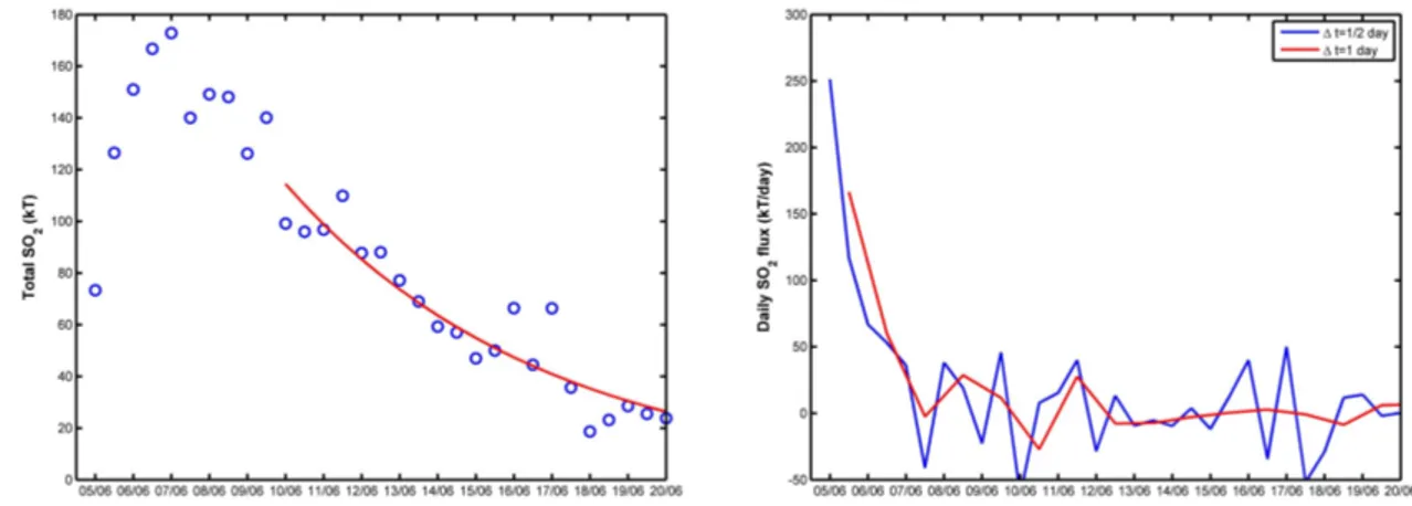
As mentioned in Sect. 3, a prerequisite to any SO2 flux calculation is the evaluation of the SO2 loss term. For this purpose, it is useful to look at the retrieved total SO2mass as a function of date as displayed in Fig. 2 (left plot).

The time series of SO2, here assuming a plume height of 13 km, shows an increase in mass in the first three days af-ter the start of the eruption and then exhibits a decrease as a result of the progressive oxidation of SO2. After 10 June,

Fig. 2. (Left plot) Time series of SO2total mass measured with IASI for the 2011 eruption of Puyehue-Cord´on Caulle (blue dots). The red curve is an exponential function fitted to the data (e-folding time: 6.8 days). A plume height of 13 km is assumed. (Right plot) Daily SO2 fluxes calculated with the delta-M method applied to the total SO2mass time series estimated on a half-daily and daily basis.

the eruption was continuing but as a result of their low in-tensity and altitude these emissions were below the detection limit of IASI retrievals. We fitted an exponential function to the decay observed at the tail of the total SO2mass curve re-sulting in an estimated e-folding lifetime of 6.8 days, typical for a dry atmosphere. Note that as the plume dilutes, parts of the plume will drop below the detection limit, so that the real e-folding lifetime is probably a bit longer than what we estimate here.

From the SO2mass time series, we then applied the delta-M method (Sect. 3.3) yielding SO2 fluxes averaged over a time interval 1t (Eq. 6). The results are displayed in Fig. 2 (right plot) for half-daily and daily mass estimates (1t = 1/2 or 1 day). Note that the flux estimates for the first half-day and first day have been calculated using a time interval of 7 and 19 h, respectively (instead of 12 and 24 h), as it is more in line with the actual time between the start of the eruption and the first observations. One can see in Fig. 2 that sometimes negative fluxes are returned and that the fluxes time series are quite noisy (especially for the half-daily estimates). This is because the method relies on accurate estimates of consec-utive SO2masses, which can be problematic for large and dispersed plumes. The erratic behavior of the half-day fluxes on 17 and 18 June is for instance due to the method used for a.m./p.m. differentiation which for these days causes por-tions of the plume to be counted twice. This behavior disap-pears when looking at the daily flux.

In addition to the simple delta-M method, Puyehue-Cord´on Caulle was found to be an ideal case study to test the traverse method (Sect. 3.2) because of the modest SO2 loss term and because the SO2injection occurred in a strong and well constrained wind field leading to steady and almost one-dimensional plumes (see Fig. 3). The analysis was made for a sequence of four consecutive SO2images right after the start of the eruption; each time, the traverses were defined for a well-chosen portion of the plume (close to the volcano).

Following the traverse method formulation (Eq. 4), we cal-culate the SO2fluxes using the MERRA wind fields (avail-able at http://disc.sci.gsfc.nasa.gov/giovanni/overview/) ex-tracted at the location of the volcano and the time of observa-tions. It allows us to reconstruct a high-resolution chronology of the SO2 flux during the eruption (Merucci et al., 2011). This is shown in Fig. 4, where the results from four consec-utive IASI snapshots (4 June p.m. to 6 June a.m.) are dis-played.

A striking feature is the fairly good overlap of the flux data for two successive overpasses, in spite of the constant wind field used in the calculation (for each IASI image). This clearly strengthens the adopted approaches. Note that for the first overpass, larger (and also more scattered) values are ob-served; this is probably due to the impact of ash (high con-centrations in the early plume) on the retrieved values.

Compared to the delta-M method (also shown on Fig. 4, for 1t = 1/2 day), results from the traverse method provide more information on the temporal variations of the emis-sions, in particular the peak occurring about 6 h after the be-ginning of the eruption, not seen with the lower time res-olution delta-M method. However, on average, the delta-M and traverse methods give values that are consistent with each other: ∼ 180 kT day−1 on the first day then dropping to ∼ 60 kT day−1on the second day.

In order to consolidate the flux results of Fig. 4, we have also applied the inversion modeling method (Sect. 3.4) to the Puyehue-Cord´on Caulle event. Since the injection heights are reasonably well known, we have used a small number of at-mospheric layers but worked at a high temporal resolution. More precisely, emission grid cells have been defined as 3 layers of 1 km thickness from 11 to 14 km and 2-hourly in-tervals for the period 4–7 June 2011, starting at the onset of the eruption. The FLEXPART simulations extended over 3 days after each release period and the results are given on a 0.5◦×0.5◦ output grid. Following the description in

Fig. 3. SO2 columns from IASI measurements for 6 June 2011 (morning overpass) over the Puyehue-Cord´on Caulle volcano. The lines correspond to the different traverses used for the SO2fluxes calculation. A plume height of 13 km is assumed. The Puyehue-Cord´on Caulle volcano is marked by a black triangle.

Sect. 3.4, a plume age dependent correction is applied using an e-folding time τ of 6.8 days (Fig. 2). The measurement vector y (Eq. 8) is assembled with the SO2 columns mea-sured by IASI (> 1 DU) for the period between 4 and 9 June 2011 (daytime and nighttime overpasses) and evaluated on the output grid. The vertical column calculation is made as-suming a plume height of 13 km. For the a priori emissions, a single value of 5 kT/2 h of SO2is used for each emission grid cell to form xa. The a priori covariance matrix Sa has been chosen as diagonal with values corresponding to 250 % errors on the a priori emissions. For the observation error co-variance matrix Sε, a diagonal matrix has been chosen and we assumed a conservative 50 % + 1 DU uncertainty on the measurements.

The inversion results are displayed in Fig. 4 (grey bars), where the a posteriori emissions have been vertically inte-grated and scaled to yield SO2fluxes. Overall, the results of Fig. 4 are very positive as they show that, for the case of Puyehue-Cord´on Caulle, it is possible to resolve the volcanic SO2emissions with a time step as short as ∼ 2 h. One can see that there is a very good correspondence between the re-sults of the traverse and inversion modeling methods, which strengthens both approaches.

By integrating the fluxes of Fig. 4, we estimate the total SO2 mass released by Puyehue-Cord´on Caulle during the first two days of eruption to be about 200 kT. However, this estimate is a lower bound as it does not include the contribu-tion of SO2emitted at lower altitude.

As an illustration of the inversion modeling method, Fig. 5 shows daily SO2column maps retrieved from IASI and

sim-Fig. 4. SO2flux evolution through the first two days of the Puyehue-Cord´on Caulle eruption obtained from the traverse method (analy-sis of four consecutive IASI images) and compared to the delta-M (1t = 1/2 day; pale orange bars) and inversion modeling methods (grey bars).

ulated by FLEXPART using the retrieved emissions (K · ˆx), for 6 and 7 June 2011. As can be seen, a fair agreement is found between IASI and FLEXPART both for the dispersion patterns and the absolute SO2column values.

4.2 Nyamulagira

Nyamulagira (1.41◦S, 29.20◦E, 3058 m a.s.l.) erupted over 40 times in the last century, and is known to be one of the main sources of volcanic SO2worldwide (Carn et al., 2003). Based on TOMS measurements, the SO2 output from Nya-mulagira has been monitored during the 1979–2005 period, and a majority of eruptions produced more than 0.8 MT of SO2(Bluth and Carn, 2008).

Almost two years after the last eruption of 2–29 January 2010, Nyamulagira started erupting again, on 6 November 2011 (18:45 UTC) with observed lava fountains reaching up to 300 m and with large amounts of SO2easily detected from space. The eruption lasted five months, until 15 March 2012. For several weeks, the plume of SO2 was monotonically drifting westward from the volcano (as illustrated in the inset in Fig. 6); its altitude was between 4 and 8 km (based on wind direction data from ECMWF).

We investigated the 2011–2012 Nyamulagira eruption for the first month (when the signal was the strongest) using the UV sensors (OMI and GOME-2) as they are the most suitable to monitor this event owing to their good sensitivity down to the surface. A strong signal of SO2 could also be detected with IASI especially at the beginning of the eruption, but the data are more difficult to use because of increasing errors on the columns with decreasing plume altitude (the plume of SO2was low in the atmosphere).

Fig. 5. SO2columns measured by IASI (evening overpasses) and simulated by FLEXPART using the a posteriori emissions from the inversion for 6 June 2011 (left panels) and 7 June 2011 (right panels). The measured columns are averaged over the 0.5◦×0.5◦FLEXPART output. The simulated columns are (1) calculated from the SO2profiles weighted by the corresponding altitude-dependent measurement sensitivity functions (averaging kernels) and (2) interpolated at the time of observations. The Puyehue-Cord´on Caulle volcano is marked by a black triangle.

Fig. 6. OMI daily SO2mass as function of plume age (see text) av-eraged for November 2011. The inset shows the monthly avav-eraged SO₂columns measured by OMI above Nyamulagira for November 2011.

Since the plume altitude is not known exactly, we sim-ply took the available middle tropospheric altitude (center of mass heights of 6 and 7.5 km for GOME-2 and OMI, respectively) for the SO2 vertical column calculation. This assumption is a source of uncertainty but the effect on the SO2 columns is modest, with errors lower than 30 % (Fig. 1). In order to isolate the volcanic SO2signal from the background noise, an SO2 column threshold was assigned (VC > VClim=VC+3·σVC), using the mean (VC) and stan-dard deviation (σVC)of daily SO2VCs retrieved in the back-ground region (Carn et al., 2008).

As already mentioned, the SO2plumes from Nyamulagira had a rather simple geometry owing to fairly stable meteo-rological conditions. This situation facilitates the calculation of the loss term (see e.g., Beirle et al., 2011) and of the SO2 fluxes. The first loss term has been estimated from the decay observed in the total SO2mass downwind (westward) of the volcano. This is illustrated in Fig. 6 showing the averaged SO2 mass for November 2011 as a function of plume age, expressed in hours.

The values are calculated using daily OMI SO2 columns integrated along traverses perpendicular to the wind vector. The plume age is the ratio of the distance (defined as pos-itive downwind) between a given pixel and the volcano and the wind speed. For each day, the wind vector is derived from

Fig. 7. Time series of SO2total mass measured with OMI for the 2011 eruption of Nyamulagira. Shown are the daily values (grey), 5-day moving averages (black) and a skewed shape function fitted to the smoothed curve (red).

the visual analysis of the transport direction of the plume and comparison with the 1◦×1◦ECMWF 24 h averaged profile (closest to the volcano) of wind direction and speed. From Fig. 6, the fitting of an exponential function (red curve) to the SO2mass data is straightforward and yields a mean SO2 e-folding time of 22.5 h, in good agreement with the litera-ture (Bluth and Carn, 2008). Moreover, we repeated the same analysis using GOME-2 data and obtained a consistent value of 24.9 h.

Having reasonably accurate values of the SO2 loss term for both OMI and GOME-2, we can estimate the fluxes using some of the methods described in Sect. 3. We start to apply these methods to the data from OMI as it is the instrument with the most favorable spatial resolution and noise level.

We first used the delta-M method. Similarly to the analysis of the Puyehue-Cord´on Caulle eruption, it is applicable to the daily SO2mass values (Fig. 7, grey bars) and does not require information on the daily wind fields.

We also tested the skewed shape method (Sect. 3.3). Since it implies the adjustment of a continuous and regular func-tion (Eq. 7), we applied this method to the (smoothed) 5-day moving averages SO2mass time series (Fig. 7, black stems with the fitted curve in red).

The resulting fluxes are shown in Fig. 8 for both methods. Also shown in Fig. 8, are the results from the box (Sect. 3.1) and traverse (Sect. 3.2) methods. For the box method, we selected the days for which the SO2plume had a simple geometry, was well covered by the satellite instru-ment and when the wind speed was not anomalously high or low. We calculated a daily flux (Fig. 8, blue bars) based on the data contained in a circle around the volcano, with a radius changing each day depending on the wind speed.

Fig. 8. Daily SO2fluxes derived from different methods applied to OMI data for the first month of the 2011 eruption of Nyamulagira.

For the traverse method, daily values (Fig. 8, pink squares) were calculated whenever possible by averaging the fluxes over the closest five to ten traverses (excluding the first one because of sub-pixel dilution issues). Note that the recon-struction of short-term variations of the flux, as for Puyehue-Cord´on Caulle, was found difficult. Short and variable SO2 lifetime, as well as a poorly constrained wind field far away from the volcano makes this kind of approach too uncertain in this case.

In general, the retrieved SO2 fluxes from the different methods are found to be in reasonable agreement, all show-ing large values (40–230 kT day−1) for the first week of the eruption and then a flattening afterwards (10–30 kT day−1) reflecting a calmer eruptive regime. In total, we estimate the SO2amount produced by Nyamulagira during the first month of eruption to be of about 1 MT.

Compared to the other methods, the delta-M method shows more variable and uncertain results. This is mainly because the plume is often not completely covered by OMI for two consecutive days. Now comparing the results of the skewed shape, box and traverse methods, the differences ob-served can be explained by small differences in selection of data, details in the settings and uncertainties on the wind speed.

To consolidate the results, we also analyzed the GOME-2 SO2data using the same techniques as for OMI. The results are displayed in Fig. 9, together with the OMI fluxes. Only the data from the circle and skewed shape methods are shown for better readability.

A general consistency is found between OMI and GOME-2 results, although GOME-GOME-2 has a tendency to produce higher values than OMI (probably because of differences in the treatment of clouds in the retrievals and in meteorological conditions). As these results are in principle independent of

Fig. 9. Time series of Nyamulagira SO2fluxes retrieved from the box (bars) and skewed shape (lines) methods applied to OMI and GOME-2 data.

the pixel size, they constitute however a valuable element of successful satellite–satellite comparison, complementing ex-isting SO2flux comparison exercises (e.g., Campion, 2011; and Campion et al., 2012).

Finally, it is important to note that, at the beginning of the event, the SO2 fluxes (Figs. 8, 9) could be underestimated because of SO2absorption saturation. However, from the in-spection of the SO2column values, we believe the effect on the fluxes is small, with differences lower than 10 %.

In an attempt to ascertain a reasonable uncertainty on the derived fluxes, we conducted sensitivity tests by vary-ing the different important parameters of the retrieval. Based on these sensitivity tests, a typical error for both OMI and GOME-2 estimates is of about 50 %, and includes the uncer-tainties on the SO2columns, cutoff values used, SO2losses and wind fields.

4.3 Nabro

Nabro (13.37◦N, 41.70◦E, 2218 m a.s.l.) is located in the African rift zone at the border between Eritrea and Ethiopia. In spite of no reported historical eruptions, Nabro erupted in the evening of 12 June 2011 around 20:30 UTC, expelling a powerful plume composed of enormous amounts of steam and SO2, with little amounts of ash. At the beginning of the eruption, SO2was massively injected at tropical tropopause levels where fast easterly jet winds (∼ 30 m s−1) transported the plume towards the Mediterranean Middle East and, later, to China. Less powerful, the next phase of the eruption in-jected SO2 at lower altitudes but still the dispersion of the plume occurred over a large part of the African continent.

The eruption led to a ∼ 20 km-long lava flow in less than ten days (see http://earthobservatory.nasa.gov/). It lasted about one month; remnants of volcanic SO2 could still be

observed by the UV sensors on 17 July 2011. The compar-ison of satellite UV and TIR SO2images revealed inhomo-geneous multi-layered SO2plumes dispersed over large dis-tances, making the SO2 fluxes calculation a complex prob-lem to solve. Therefore we have used a more elaborated ap-proach: the inverse modeling method (Sect. 3.4).

Note that Nabro is a difficult event to analyze as – un-like the Puyehue-Cord´on Caulle (explosive) and the Nyamu-lagira (effusive) eruptions discussed above – it fundamen-tally was an effusive eruption releasing an exceptional gas jet that reached the tropopause prior to strong lava emis-sion. As there is no evidence that this plume was ash laden as would be expected of a high altitude plume, Nabro re-mains an intriguing, atypical example in this respect. The transport mechanism of the initial Nabro eruption plume is also peculiar. Bourassa et al. (2012) have suggested deep convection associated with the Asian monsoon circulation to explain the strong impact of the eruption on the strato-spheric aerosol loading. However, this mechanism is contro-versial after Vernier et al. (2013) and Fromm et al. (2013) provided satellite evidence for direct injection of the initial Nabro plume into the lower stratosphere.

4.3.1 Inversion settings

The inversion of the time-dependent SO2emission profiles is based on the maximum a posteriori solution described in Sect. 3.4 (Eq. 10). The emission grid cells are defined as: 16 layers of 1 km thickness from 2 to 18 km altitude and 64 6-hourly intervals for the period 13–28 June 2011, plus an addi-tional profile to cope with the plume for the very first hours of the eruption (12 June – 20:30 UTC to 13 June – 00:00 UTC). The inversion consists in estimating the SO2masses that have been emitted in each of these grid cells. In line with Eq. (8), we define a state vector x that gathers all the n = 1040 un-known emissions.

The FLEXPART simulations extended over 5 days after each release period and the results are given on a 1◦×1◦ output grid. As mentioned in Sect. 3.4, concentrations are in-terpolated in space and time with the satellite measurements (see below), multiplied by the corresponding SO2averaging kernels (to allow direct comparisons with satellite measure-ments) and vertically integrated to provide columns. For the present study, we have applied a correction for SO2loss us-ing a τ value different for each emission layer. From the de-cay observed in the total SO2mass after the end of the first major injection episode (not shown), we derive an e-folding lifetime of 5 days for the high altitude plumes at 15–18 km (Vernier et al., 2013; Fromm et al., 2013). The e-folding time parameterization as a function of altitude was estimated by interpolation between the values at surface level, taken as 2 days, and the one at 15–18 km (5 days). The value of the SO2 e-folding time at the surface has been varied until the best match was found between the measurements and the simula-tions.

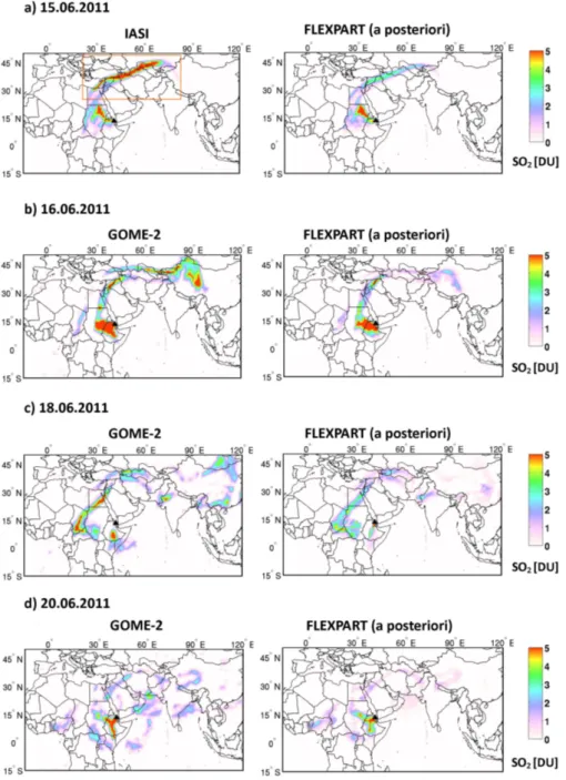
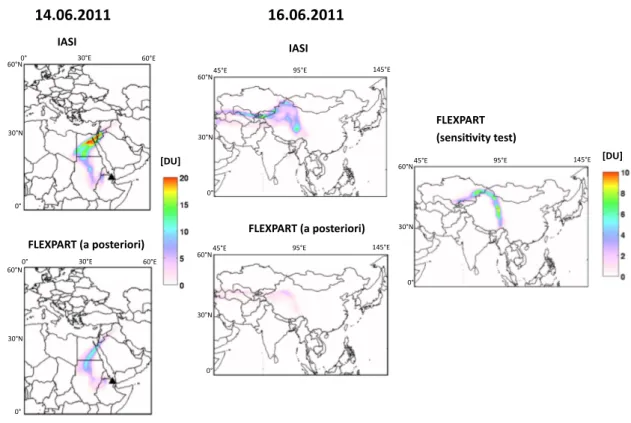
Fig. 10. SO₂columns measured by IASI (morning overpass) and GOME-2 and simulated by FLEXPART using the a posteriori emissions from the inversion for 15 June 2011 (a), 16 June 2011 (b), 18 June 2011 (c) and 20 June 2011 (d). The measured columns are averaged over the 1◦×1◦FLEXPART output grid. The simulated columns are (1) calculated from the SO₂profiles weighted by the corresponding altitude-dependent measurement sensitivity functions (averaging kernels) and (2) interpolated at the time of observations. The Nabro volcano is marked by a black triangle. The orange box shows the SO2plume released in the first 15 h of the eruption.

The observations used to build the measurement vector y (Eq. 8) are the SO2columns measured by IASI (daytime and nighttime overpasses) and GOME-2 for the period between 13 June and 3 July 2011, evaluated on the output grid. Note however that the GOME-2 measurements for 14 June 2011 have not been considered in the analysis because the instru-ment was operating in its narrow swath mode on that day.

As a baseline, the calculation is made for SO2 columns larger than 1 DU and assuming a plume height of 16 km for both sensors. Hence the averaging kernels by definition equal 1 at this altitude.

To solve the inversion problem (Eq. 10), several other variables need to be specified: the a priori state vector (xa), the error covariance matrices of the a priori (Sa)and of the measurements (Sε). For the a priori emissions, we

have estimated first-order SO2flux from the skewed shaped method (Sect. 3.3) applied to the global SO2total mass time series from GOME-2 (i.e., with a measurement sensitivity to SO2 down to the surface). For each day, the inferred SO2 mass was then distributed equally in each emission grid cell to form xa. The a priori covariance matrix Sa has been cho-sen diagonal with values corresponding to 250 % + 2 kT er-rors on the a priori emissions, except in the layers below 6 km where a larger uncertainty was used (2000 % + 10 kT of the a priori emissions). Based on sensitivity tests, these settings were adopted to avoid an inversion over-constrained by the a priori values because of reduced sensitivity to SO2in the lower troposphere. For the observation error covariance ma-trix Sε, a diagonal matrix has been chosen and we assumed a conservative 50 % + 1 DU uncertainty on the measurements. Note that we tested the sensitivity of the inversion to the ob-servation error covariance matrix Sε and it was found to be reasonably small.

4.3.2 Results

From inspection of the SO2column distributions, it appears that the GOME-2 and IASI data are quite similar, but the sequence of SO2images also shows differences that can be attributed (at least partly) to plumes of SO2at different al-titudes. In principle, the inversion scheme exploits the in-strumental complementarities to resolve the injection pro-files in the altitude range extending from the surface to the lower stratosphere. At the beginning of the eruption, SO2is massively injected at high altitudes and the IASI retrieval is found to be optimal, owing to its large column applicability and 12 h revisiting time (as opposed to 24 h for GOME-2). Shortly after the first injection episode, SO2is more evenly distributed throughout the atmosphere, conditions for which GOME-2 provides information on the total atmospheric SO2 column, including the contribution from the lower tropo-sphere (not probed as efficiently by IASI). Note that after the first week of the eruption, the IASI SO2signal close to Nabro is quite small, indicating low altitude SO2plumes and hence most information on the emissions is brought by the GOME-2 data.

Before inspecting the inverted fluxes, let us first compare the SO2columns retrieved from GOME-2 or IASI and sim-ulated by FLEXPART using the retrieved emissions. As an illustration, Fig. 10 shows daily SO2maps for 15, 16, 18 and 20 June 2011.

Generally the simulated SO2vertical columns agree fairly well with the observations. However, it should be noted that the strong SO2plume released at the beginning of the erup-tion, which then moves towards East Asia, is not well repro-duced by the simulations. This plume was injected at high altitudes in the first 15 h of eruption. The reasons for this dis-crepancy will be investigated in Sect. 4.3.3. Nevertheless, the overall good agreement between the observed and modeled SO2columns for the other plumes suggests that it is neither

Fig. 11. Comparison of SO2flux estimates for the eruption of Nabro using different methods. Upper panel: vertically integrated a pos-teriori emissions from the inversion combining IASI and GOME-2 data (dark grey bars: > 6 km; light + dark grey bars: total flux), flux estimate of the early plume using the box method applied to IASI (orange bar; see text and Fig. 10a), results of the skewed-shape method applied to GOME-2 data and used as a priori in the inversion (blue dotted line; z: 16 km), results of the delta-M method applied to IASI data (magenta and red lines for half-daily and daily mass estimates; z: 16 km) and results of the traverse method applied to MODIS (cyan squares). Lower panel: same as upper panel (but with a focus on the first four days of eruption) with flux results of the traverse method for three IASI images at the beginning of the eruption.

a serious nor a general problem. From Fig. 10, one can also see that not all plume maxima are well captured. This points to limitations in the approach used (in terms of spatial and time resolution) to capture the complexity and details of the emissions (Eckhardt et al., 2008).

The flux estimates are displayed in Fig. 11 (upper panel), where the a posteriori emissions have been integrated