Detecting medium changes from coda by interferometry
Oleg V. Poliannikov∗and Alison Malcolm, Earth Resources Laboratory, MIT
SUMMARY
In many applications, sequestering CO2 underground for ex-ample, determining whether or not the medium has changed is of primary importance, with secondary goals of locating and quantifying that change. We consider an acoustic model of the Earth as a sum of a smooth background velocity, isolated ve-locity jumps and random small scale fluctuations. Although the first two parts of the model can be determined precisely, the random fluctuations are never known exactly and are thus modeled as a realization of a random process with assumed statistical properties. We exploit the so-called coda of multi-ply scattered energy recorded in such models to monitor for change and to localize and quantify that change, by examining the shape and frequency content of correlations of the coda produced by different parts in the medium. These ideas build upon past work in time-reversal detection methods that have often been limited to theoretical regimes in which the scales of scattering and reflection are strictly separated. This results in an application of time-reversal detection methods to non-theoretical regimes in which the separation of scales is not strictly satisfied, opening up the possiblity, discussed here, of using such techniques to monitor CO2sequestration sites for leakage.
INTRODUCTION
Detection and characterization of changes in the Earth’s sub-surface is important for a variety of energy-related applications including enhanced production from petroleum reservoirs, the development of Enhanced Geothermal Energy Reservoirs, and the sequestration of Carbon Dioxide as part of a Greenhouse gas reduction effort. The gold standard for detecting such changes is 4D seismic. Lumley (2001) presents a relatively recent review of general 4D technology and Lumley (2010) gives an overview of the current state of the art as applied to CO2monitoring.
For the smaller budgets of geothermal and CO2efforts, 4D is too expensive to be used as a continuous monitoring technol-ogy. Cheaper but possibly cruder change detection algorithms could be used as alarms that would trigger a full size survey only when it is strongly suspected that a significant change in the subsurface has occurred.
In realistic environments, seismic waves propagate through com-plex media. The recorded signals are therefore also compli-cated. Most imaging algorithms designed for such media rely on the availability of the direct reflection from the non-random structure one is trying to image (Borcea et al., 2005, 2006). It is not always possible in practice to separate coherent re-flections like this from surrounding multiply-scattered energy. Furthermore, the multiply-scattered “noise” itself may contain useful information about the subsurface that could be used as
a basis for a detection algorithm.
Lumley et al. (2008) report that injecting CO2 generates a strong coda of multiply-scattered energy, and that this coda changes significantly, even in synthetic data, before and af-ter CO2injection. This indicates that methods exploiting this coda are promising for low-budget monitoring. Significant progress on these sorts of methods has been made recently, such as the development of the so-called coda wave interfer-ometry method (Poupinet et al., 1984; Snieder et al., 2002) in which multiply-scattered coda is used to estimate, with high precision, a time delay indicative of a change in the bulk sound speed of the medium. Zhou et al. (2010) show that this type of method can be used to monitor for change in a CO2 reser-voir, without placing receivers in the reservoir interval. A similar technique, coupled with the recovery of the Green’s function from noise sources, has been proposed in (Brenguier et al., 2008a,b) as a passive monitoring method. Although these methods provide valuable information about bulk changes in the medium, they are not naturally able to isolate and quan-tify the change they detect. An example of an attempt to ex-tend the coda-wave interferometry method to be able to local-ize change, through a sensitivity kernal approach, is given in (Pacheco and Snieder, 2005). Here, we present a method that allows us to both localize the change, through a tomography-like procedure, and to quantify the change, specifically to de-termine whether the (assumed to be) random velocity perturba-tions that generate the multiply-scattered coda grow or shrink. In one-dimensional media in which the scales of scattering, frequency, and recording lengths are strictly separate, there are theoretical results that detail the estimation of the aver-age size of scatterers in a region and the 1D location of that region (Fouque and Poliannikov, 2006). Our present work is a first step in the generalization of these methods beyond sit-uations in which these assumptions are strictly satsified. The resulting estimator works by examining the frequency content of the auto-correlation of the coda, using the evolution of this frequency content over the recording time to track the loca-tion and size of scatterers. Changes in the evoluloca-tion of the frequency content as a function of recording time between the initial and monitor surveys is then indicative of change in the reservoir. The resulting estimator is statistically stable, sensi-tive to the type of change, i.e., increase or decrease in scatterer size, and able to localize the change, given the average back-ground velocity.
METHOD
Problem setup and motivation
We describe our experiment in terms of the problem of CO2 sequestration. However, our methodology and conclusions ex-tend beyond this particular application to more general prob-lems so long as they conform to the same basic mathematical
Figure 1: Initial model setup. A single source and a single receiver are placed on the surface at the origin.
framework. In this framework, we suppose that we have a two-dimensional acoustic medium consisting of a velocity field that is a superposition of a smooth macroscopic background and random fine scale perturbations. In our numerical experiments (Figure 1), the initial background velocity is fixed at 3000 m/s. We do this for simplicity, our method does not require that the background velocity model be known. The perturbations to this 3000 m/s are modeled as a realization of a Gaussian ran-dom field with correlation length 5 m.
We consider a single source zero-offset experiment, with the source/receiver located at the surface. The source emits a Ricker wavelet pulse with central frequency 30 Hz. As the wave prop-agates downward, the inhomogeneities in the background ve-locity produce reflections. These reflected waves form a ran-dom coda that is recorded at the surface and is a function of the velocity perturbations inside the medium. A particular re-alization of the velocity perturbations cannot be known and is actually of little interest. Our focus is rather on the overall large scale statistical properties of the random field. If those properties have changed in a particular region, we would like to detect that change based on the observed coda reflections. In what follows, we consider two mathematical models for the change in scattering properties and propose a method to detect that change and even quantify it.
Interferometric refocusing of coda
We will denote the recorded reflections p(t). It is well-known that the autocorrelation of the coda C(t) =` p(·) ? p(−·)´(t) contains a coherent component around zero-lag (Fink, 1999). This coherent signal consists of the autocorrelation of the source wavelet, to which a medium dependent filter is applied. In some cases it is possible to deconvolve the source from this autocorrelation leaving only the medium dependent filter. This filter can be viewed as aggregate information about the medium that was embedded in the reflections. In more general cases, when a clear separation between the contribution of the source and that of the medium is impossible, the imprint introduced by the medium dependent filter can still be analyzed to recover information about the medium.
Frequency content of reflections
Our detector of a substantial change in the scattering proper-ties of the medium is based on the frequency content of the coherent part of the autocorrelation function C(t). If T is the period of the source wavelet then we only consider C(t), where −T ≤ t ≤ T , and we taper the signal at the edges. The spec-trum of the autocorrelation depends on the nature of the scat-tering inside the medium traversed by the wave.
More specifically, we expect that the amount of reflected en-ergy in a chosen frequency band depends on the size of the typ-ical scatterer encountered by the wave; larger scatterers reflect low frequencies much better than smaller ones. This suggests a simple principle of detecting and quantifying the change in scattering in the medium. Based on the observed change in the energy distribution among different frequencies, we can deter-mine if the size of a typical scatterer inside the medium has increased or decreased.
While in principle we could be interested in the entire spec-trum of the autocorrelation, in this work we only concentrate on the dominant frequency, which we define as the frequency at which the maximal spectral amplitude of the autocorrelation occurs. From this analysis of the frequency content we obtain an estimate of the type of change in the medium, i.e., bigger to smaller scatterers or vice versa.
Expanding recording time window
In order to localize this change, we exploit the standard rela-tionship between traveltime and velocity. In other words, if the maximum velocity in the medium is vmaxthen the reflections recorded up to time Tf can only contain information about the medium with depth no greater than d = vmaxTf/2. Therefore by varying the amount of coda used for analysis, we can effec-tively probe different depths (Fouque et al., 2004; Fouque and Poliannikov, 2006). A statistically significant change in the properties of the autocorrelation of the coda detected at some fixed time is indicative of a change in the scattering properties at a corresponding distance from the source.
When strong multiple scattering is present, the precise rela-tionship between scattering statistics and the spectrum of the reflected coda is very non-trivial. With time lapse measure-ments at our disposal, we can still describe the fundamental nature of the change as our numerics show below.
Correlation length change vs velocity change
To understand the relationship between changing the correla-tion length and changing the macroscopic velocity, we sup-pose that the velocity perturbations are caused by randomly placed ideal point scatterers. The coda recorded in time is then a superposition of multiply scattered randomly delayed diffractions. By increasing the spacing between the individ-ual diffractors we increase the time between consecutive re-flections. We could achieve the same effect by decreasing the macroscopic velocity in the scattering region. Fouque and Po-liannikov (2006) show that change in the correlation length of the velocity perturbations manifests itself in the same way as change in the macroscopic velocity inside the same region. In the following section, we explore both ways to model the change in scattering properties.
NUMERICAL EXAMPLES
As was discussed in the previous section, we assume that we have a medium with a constant background and random ve-locity perturbations. We will assume that CO2 is injected to the subsurface, which alters the medium inside one layer. We would like to show that such a change can be detected from the surface. To this end, we perform three experiments, described in the following three subsections.
Different realization of medium with the same statistics First, we assume that the injection of the CO2 has resulted in a new realization of velocity perturbations with the same statistical properties. The injection layer extends from 1500 to 2000 m. The two-way travel time to the top of the layer and back to the surface is about 1 s. We see in Figure 2 that the two codas before and after the injection are identical before 1 s and they deviate afterwards.
We now fix the beginning of the cut-off window at 0.3 s and continuously vary the end point from 0.5 to 2 s. For each win-dow, we autocorrelate the coda, cut the autocorrelation around zero-lag, transform it to the Fourier domain and record the fre-quency with the maximum amplitude.
Figure 3 shows that although the two codas are point-wise dif-ferent, their frequency content is nearly identical. We therefore conclude that the statistical properties of the medium were not changed by the injection. This indicates that our method is statistically stable.
Figure 2: The medium between depths 1500 and 2000 m is replaced with another random realization with the same statis-tical properties. Dashed line marks the time when the codas recorded before and after the change deviate.
Different correlation length
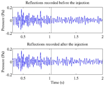
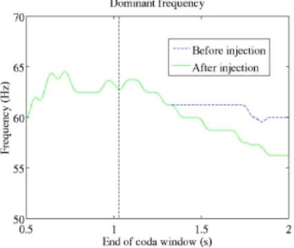
We now suppose the injection has changed the statistical prop-erties of velocity perturbations. This is more realistic as we would expect CO2injection to have a deterministic effect on the medium properties. Specifically, we assume that after the injection the correlation length inside the same layer (between 1500 and 2000 m) has increased from 5 to 25 m (Figure 4). As in the previous example, the reflected coda is identical up to a time of 1 s (Figure 5). However, the dominant frequency as a function of the recording window exhibits a completely differ-ent behavior. The injection has resulted in more low frequency
Figure 3: The two signals in Figure 2 (from before and after the change) do not show significant differences. This shows the statistical stability of the method.
energy being reflected (Figure 6), which allows us to conclude that the correlation length in the layer has increased.
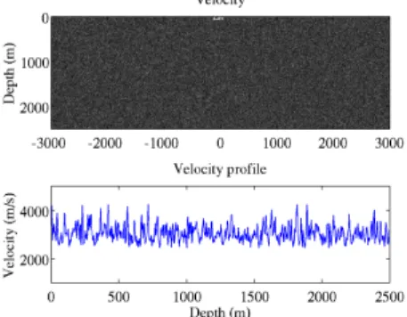
Figure 4: We model the injection as a local change in the cor-relation length of random perturbations for depths in the range 1500 ≤ z ≤ 2000 m.
Figure 5: The reflected signal before and after the change in scattering (Figure 4). The time when the the codas deviate is marked with a dashed line.
Different macroscopic velocity
We now assume that the injection of CO2 has resulted in the change of the macroscopic velocity. Accordingly, the back-ground velocity inside the injection layer is reduced to 1600 m/s while the velocity perturbations remain unchanged from the
Figure 6: These dominant frequencies are obtained from codas in Figure 5. Lower dominant frequency means bigger scatter-ers. Thus we can infer from the change in frequencies that the layer contains larger scatterers, which is correct for the intro-duced model change.
pre-injection state. We use a 50 Hz Ricker source for this setup. We have increased the frequency of the source pulse so that we are able to detect changes of this magnitude. Al-though this change remains much larger than we would expect to see in practice, through a combination of stacking of mul-tiple recordings and incorporating additional frequency infor-mation smaller contrasts should be detectable. We note that the arrival from the newly formed boundary between the layers is completely buried in the random coda (Figure 8). However, by looking at the dominant frequency (Figure 9), we can see the change in the scattering properties of the medium after 1 s.
Figure 7: Background velocity is changed to 1600 m/s inside the layer.
CONCLUSIONS
Detection of change in a complex medium is an important problem. While large 4D seismic surveys remain an impor-tant tool, devising an inexpensive alarm that can be triggered if a considerable change in the subsurface has occurred has great practical benefits. In the context of CO2sequestration, it may aid in sequestration monitoring as well as help detect any potential leaks.
Despite many recent advances, the scattered coda is still often
Figure 8: Reflections corresponding to the model before and after the change described in Figure 7.
Figure 9: The dominant frequency as a function of the coda window once again shows that the scattering in the layer has changed. Lower velocity is equivalent to a larger correlation length.
viewed as noise and discarded. We provided further evidence that it may contain important information about the subsur-face that methods based on coherent arrivals fail to extract. We have shown that, in a multiply scattered medium, by vary-ing the recordvary-ing window, we can probe different depths and not only detect but also localize the change in the scattering properties inside the medium, using the change in frequency content of the coda. While finding a simple method for di-rectly inverting the spectrum of the autocorrelation remains a challenge, our numerical experiments show that the decrease in the dominant frequency is caused either by an increase in the correlation length of the velocity perturbations, or equiva-lently, by a decrease in the background velocity.
ACKNOWLEDGEMENTS
We thank both Michael Fehler and Daniel Burns of ERL for their valuable input. This work has been supported by the ERL Founding Members Consortium.
REFERENCES
Borcea, L., G. Papanicolaou, and C. Tsogka, 2005, Adaptive interferometric imaging in clutter and optimal illumination: Inverse Problems, 21, 1419–1460.
——–, 2006, Coherent interferometry in finely layered ran-dom media: SIAM Journal on Multiscale Modeling and Simulation, 5, 62–83.
Brenguier, F., M. Campillo, C. Hadziioannou, N. M. Shapiro, R. M. Nadeau, and E. Larose, 2008a, Postseismic Relax-ation Along the San Andreas Fault at Parkfield from Con-tinuous Seismological Observations: Science, 321, 1478– 1481.
Brenguier, F., N. M. Shapiro, M. Campillo, V. Ferrazzini, Z. Duputel, O. Coutant, and A. Nercessian, 2008b, Towards forecasting volcanic eruptions using seismic noise: Nature Geosci, 1, 126–130.
Fink, M., 1999, Time-reversed acoustics: Scientific American, 281, 91–97.
Fouque, J., J. Garnier, A. Nachbin, and K. Solna, 2004, Imaging of a dissipative layer in a random medium using a time-reversal method: Presented at the Proceedings of MC2QMC, Springer.
Fouque, J.-P., and O. V. Poliannikov, 2006, Time reversal de-tection in one-dimensional random media: Inverse Prob-lems, 22, 903–922.
Lumley, D., 2010, 4d seismic monitoring of CO2 sequestra-tion: The Leading Edge, 29, 150–155.
Lumley, D., D. Adams, R. Wright, D. Markus, and S. Cole, 2008, Seismic monitoring of CO2geo-sequestration: real-istic capabilities and limitations: SEG Technical Program Expanded Abstracts, 27, 2841–2845.
Lumley, D. E., 2001, Time-lapse seismic reservoir monitoring: Geophysics, 66, 50–53.
Pacheco, C., and R. Snieder, 2005, Time-lapse travel time change of multiply scattered acoustic waves: Journal of Acoustical Society of America, 118, 1300–1310.
Poupinet, G., W. L. Ellsworth, and J. Frechet, 1984, Mon-itoring velocity variations in the crust using earthquake doublets. An application to the Calaveras fault, California: Journal of Geophysical Research, 89, 5719–5731. Snieder, R., A. Grˆet, H. Douma, and J. Scales, 2002, Coda
wave interferometry for estimating nonlinear behavior in seismic velocity: Science, 295, 2253–2254.
Zhou, R., L. Huang, J. T. Rutledge, M. Fehler, T. M. Daley, and E. L. Majerc, 2010, Coda-wave interferometry anal-ysis of time-lapse VSP data for monitoring geological car-bon sequestration: International Journal of Greenhouse Gas Control. (in press).