An analysis of a continuum X-ray Diffraction/Fluorescence instrument

(1)

An Analysis of a Continuum X-ray Diffraction/Fluorescence Instrument by

Caitlin A. Murphy

Submitted to the Department of Earth, Atmospheric and Planetary Sciences in Partial Fulfillment of the Requirements for the Degree of

Bachelor of Science in Earth, Atmospheric and Planetary Sciences at the Massachusetts Institute of Technology

June 1, 2007

The author hereby grants to M.I.T. permission to reproduce and distribute publicly paper and electronic copies of this thesis

and to grant others the right to do so.

Author

Signature redacted

U'

Certified

by-Accepted by

I U _{Department of Earth, Atmospheric and Planetary Sciences}

June 1, 2007 Sang-Heon Shim Thesis Supervisor Sam muwrin

Signature redacted

--Signature

redacted

Chair, Committee on Undergraduate Program

MASSACHUSETTS INSTITUTE OF TECHNOLOGY

OCT 2

4 2017

LIBRARIES

ABSTRACT

Scientists at NASA's Goddard Space Flight Center have developed a Combined X-ray

Diffraction/Fluorescence (CXRDF) instrument. CXRDF performs simultaneous chemical and structural analysis of an unprepared sample, making it ideal for planetary mineral identification. In an effort to analyze the effectiveness of CXRDF, samples were chosen from a list of minerals that are important in the debate about the origin of the outcrops at Meridiani Planum on Mars. These samples were run on both CXRDF and a laboratory X-ray diffractometer. The datasets were compared, looking at peak identification, d-spacing resolution, and whether the instruments could definitively identify each sample. CXRDF successfully measured the d-spacings for each mineral, and the chemical analysis data were very valuable. However, for CXRDF to be able to definitively identify minerals, its d-spacing range and resolution will need to be improved, in addition to its data analysis software.

(3)

LIST OF FIGURES

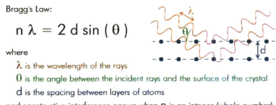
Figure 1: Bragg's Law 8

Figure 2: X-ray fluorescence 9

Figure 3: A Schematic of the specific components of CXRDF 10

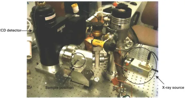
Figure 4: A Picture of CXRDF 11

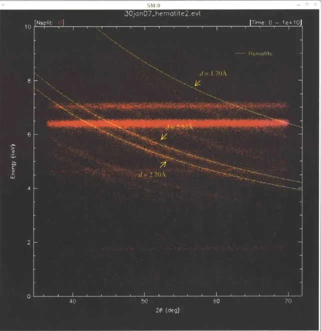
Figure 5: A plot of Energy vs. 20 for hematite 13

Figure 6: Energy vs. d-spacing plot for hematite 14

Figure 7: PANalytical data for hematite 24

Figure 8: PANalytical data for gypsum 24

Figure 9: PANalytical data for jarosite 25

Figure 10: PANalytical data for anhydrite 26

Figure 11: A plot of d-spacing vs. counts for

jarosite

28

Figure 12: A plot of Energy vs. 29 for jarosite 30

Figure 13: A plot of Energy vs. 29 for hematite 31

Figure 14: A plot of d-spacing vs. counts for hematite 32

Figure 15: A plot of d-spacing vs. counts for anhydrite 34

Figure 16: A plot of d-spacing vs. counts for gypsum 35

(5)

LIST OF TABLES

Table 1: Diagnostic Minerals of the three Theories about the Geologic History of the

Outcrops at Meridiani Planum 17

Table 2: Minerals that are Studied in this Thesis 18

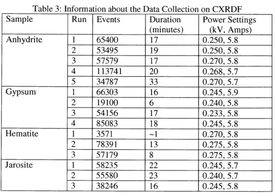
Table 3: Information about the Data Collection on CXRDF 19

(6)

I. Introduction - the Importance of a Planetary XRD

We are getting to the stage in our planetary exploration where we are looking at the geology of other planets in great detail. Although we can gain some information from satellite images that are sent back to Earth, we will not be able to clearly piece together the geologic histories of other planets unless we can identify exactly what rocks and minerals are present.

There have been a number of instruments that have attempted to shed light on the geologic makeup of planetary bodies such as the Moon and Mars. The most recent instruments employed to identify rocks and minerals on Mars are Mbssbauer Spectrometers and Thermal Emission Spectrometers. Both thermal emission spectroscopy (TES) and M6ssbauer

spectroscopy (MS) are absorption-emission techniques. In TES, when certain wavelengths of infrared radiation are absorbed by a molecule, the molecule will begin to resonate, emitting radiation of the same wavelength. The frequency of this vibration is characteristic for each molecule, and thus can be used to identify it. However, when many types of molecules are present-as in rocks and mineral-the frequencies of vibration overlap with one another, making it difficult to determine which combination of molecules would produce such a spectrum. In addition, there can be more than one combination of minerals that produces a single spectrum, making TES a non-definitive technique [1].

Mbssbauer spectroscopy is equally non-definitive. Mdssbauer spectroscopy uses a radioactive source that bombards a sample with y-rays. If the energy of these y-rays is the same as a transition energy level in the crystal, then resonant absorption will occur. This is known as the Mossbauer effect, which only works in a few isotopes. In the Missbauer spectrometers sent to Mars, the isotope that is studied is 1Fe, which limits the MS data to Fe-bearing minerals.

(7)

well-known spectra for pure minerals. However, rocks in an outcrop may have multiple iron-bearing minerals. This makes the spectrum difficult to interpret because it is impossible to know how many phases are being measured. Therefore, while both MS and TES produce data that enhance our knowledge about the composition of the rocks, they do not definitively identify the minerals that make up the rocks [2].

The instrument that will be analyzed in this thesis is an excellent alternative to MS and

TES. Dr. Keith Gendreau's instrument is a Continuum X-ray Diffraction/Fluorescence

(CXRDF) instrument. X-ray diffraction utilizes Bragg's Law to yield information about the crystal structure of a sample, while XRF is a chemical analysis tool that identifies what elements are present in the sample. This combination of chemical analysis data and structural data is an excellent way to identify rocks and minerals.

CXRDF has a number of features that make it ideal for planetary exploration. For starters, it has the huge advantage of being able to take measurements on site. We are not currently able to return samples from distant planets, and therefore the only option is to measure a rock in place. CXRDF is particularly ideal for identification on site because it does not require any sample preparation. Therefore, it does not rely on any moving parts that could possibly malfunction after landing on another planet. In addition, the combination of chemical data and structural data allows for nearly fool-proof identification of rocks. With the design of CXRDF, this can be achieved with a lightweight instrument that requires minimal power: the ultimate goal is for the instrument to weigh 2 kg and to use only an average of 2 Watts of energy [3].

CXRDF is not the only instrument of its kind. CheMin is a CCD-based XRD/XRF instrument that is scheduled to fly on the Mars Science Lab Mission in 2009. So why develop a similar instrument? We believe that CXRDF has a superior design. While CXRDF requires no

(8)

sample preparation, CheMin requires a powdered sample. Therefore, if CheMin's grinder, sieve, or sample holder were to fail, CheMin would be rendered useless [4]. In addition, CXRDF is able to identify water ice in a solid sample [3], whereas any ice within a mineral would likely evaporate when powdered by CheMin. Finally, only CXRDF is capable of acquiring

information about a sample's texture, which could be significant for determining the formation conditions of a given mineral, or what types of weathering processes it has undergone'.

The purpose of this thesis is to assess the effectiveness of CXRDF at identifying rocks and minerals. The instrument will be tested to determine whether it can identify minerals that may be important in solving one piece of the puzzle that is Mars' geologic history. After

assessing whether CXRDF is capable of identifying these key minerals, suggestions will be made for how to improve the effectiveness of the instrument.

11. The instrument A. Theory

In XRD, a sample is bombarded with X-rays of wavelength A. These X-rays are diffracted if Bragg's Law is satisfied (Figure 1) [5].

Bragg's Law:

nX

=

2d

sin

(0)

r

where Id

A. is the wavelength of the rays

0 is the angle between the incident rays and the surface of the crystal

d

is the spacing between layers of atoms

and constructive interference occurs when n is an integer (whole number)

Figure 1: Bragg's Law. X-ray diffraction is based on the constructive interference of X-rays that diffract off of planes of atoms.

This thesis will not deal specifically with CXRDF's ability to gather information about a rock's texture, but it is important to note as it is yet another capability of the instrument.

(9)

0 is the angle at which the path difference of X-rays diffracting off two planes with the same

orientation and a distance d between them is equal to an integer value of the wavelength (A), thus producing constructive interference. A detector then detects these diffracted X-rays. From the location of each event, the diffraction angle can be calculated, given the location of the sample. Also, the d-spacings-which can be calculated using Bragg's Law once 0 is known-are used to identify the sample.

CXRDF utilizes Bremsstrahlung radiation. In other words, it irradiates the sample with a continuum of wavelengths, spanning between 0.00124 and 1.24A (10.1626 to 101.626 keV) [3]. This aspect of the instrument allows for the fluorescence of certain elements. When an atom is bombarded with X-rays, there is a chance that it will absorb an X-ray. If the absorbed X-ray has sufficient energy, it will eject the innermost electron, creating a vacancy in the inner shell of the atom. This unstable situation is made stable again when an electron from an outer shell

transitions to the inner shell. During this transition, a characteristic X-ray is emitted that is equal in energy to the difference between the energy levels of the outer shell and the inner shell (Figure 2) [6]. The X-ray that is produced by the transition of the electron is then detected by the

instrument's energy-resolving CCD detector, and can be used to identify the elements that are present in the sample.

Polaledmrn E-, x-ray 0- _&EEI-Eg-K. cle euEl or 0 E₂-E₀-K~ C) ED Incoming F- x-a=y~= radiation from radioisotope.

(10)

B. Design

CXRDF is a combined X-ray diffraction and X-ray fluorescence instrument. The basic components include an X-ray source, which produces a continuum of X-rays from a gold coated target; the X-ray chamber, where X-rays are collimated so that they are all traveling roughly parallel to one another, toward a single spot on the sample; and an energy-resolving CCD camera which serves as the detector [3].

Diffracted and Fluorescence X-ray X-ray SourceBeams

Collimated X-ray Beam .

----...---' Z

Sample at (x.,y.,z.) Figure 3: A schematic of the specific components of CXRDF [3].

CXRDF is capable of simultaneously collecting diffraction and fluorescence data because it utilizes a multi-wavelength source and a charge-coupled device (CCD) detector capable of energy resolution. Detectors in traditional X-ray diffractometers measure either the diffraction angle or the wavelength of diffracted X-rays. In CXRDF, the detector can pick up both. CXRDF utilizes a commercial CCD camera, where each pixel is capable of energy resolution. Therefore, the camera captures both geometric and energy data, as it measures not only the location of each event-related to the diffraction angle-but also the energy associated with it.

(11)

CCD detector

- X-ray source

Figure 4: A picture of CXRDF, with the major features of the instrument labeled.

The X-ray source and the CCD are held in a vacuum chamber. While this adds an additional component to the instrument-a vacuum pump-it is necessary to keep any moisture off of the CCD, and to block out all external light from the CCD, since it is energy-sensitive. In addition, it ensures that the CCD detector will not be contaminated in, for example, the dusty conditions of Mars. As a result of the vacuum, the sample is separated from the X-ray source and the CCD detector by a Beryllium window. This window is virtually transparent to X-rays, although it does absorb lower-energy X-rays, thus lowering the signal. The sample-preferably a flat face-is placed flush against this window. A single spot approximately 1mm x 2mm on the sample is hit by the X-rays that come through the window. It is this part of the sample from which X-ray diffraction and fluorescence are measured.

The Beryllium window is a significant design feature of the instrument, as it affects the incident angle of the X-rays. The incident angle determines the range of d-spacings that can be detected by the instrument. From Bragg's Law, smaller incident angles correspond to larger d-spacings. However, given the design of the instrument, as the incident angle gets smaller, the

(12)

path the X-rays must take through the Beryllium window increases, which lowers the signal. Currently, the incident angle is set at 300, which means the instrument can only pick up d-spacings 4.5A. The instrument's designers are weighing the costs and benefits of lowering the angle slightly to increase the maximum detectable d-spacing to approximately 6 - 7A.

C. Data

Figure 5 shows the format of a typical dataset. Figure 5 is a plot of Energy vs. 20 for hematite (Fe2O3) A2 2 is related to energy by

he E

where h is Planck's constant (6.626x10-34 _m2_{kg/s), c is the speed of light (299,792km/s), and}

E is energy. Therefore, in a plot of Energy vs. 20, if the y-axis is the energy of the diffracted

X-ray (A) and the x-axis is the angle (9), then the slope-or the arcs-must be related to the d-spacings, since d is the only other variable. A number of arcs are identified in Figure 5 to show where certain d-spacings fall on the plot. The smallest d-spacings are in the top-right corner of the plot (large 29 and large E), and get gradually bigger as both 29 and E decrease.

A second feature of the plot in Figure 5 is the fluorescence feature. The fluorescence

lines are horizontal, representing constant energies (i.e. the characteristic energy levels discussed above) at all angles. In Figure 5, there are three horizontal lines. The lines at 6.4 keV and 7 keV correspond to the Fe Kot and Fe KO lines, respectively3_{. This is appropriate for hematite,}

2 20 _{is simply 2x the measured diffraction angle}

(0) .

3 Kux refers to an electron that falls to the K shell from one shell above, while Kp refers to an electron that falls to

(13)

whose composition is Fe203. However, the third fluorescence line at 1.74 keV corresponds to

the fluorescence of Si, which is surprising for a hematite sample4. This will be revisited later when discussing the significance of the fluorescence data.

Figure 5: A plot of Energy vs. 20 for hematite. Each arc corresponds to a d-spacing, while horizontal lines result

from X-ray fluorescence.

4 There is another horizontal line at approximately 4.7 keV. This is known as a Si-escape feature, and is an artifact of the detector that occurs with bright fluorescence lines, such as the Fe Kct line in Figure 5.

(14)

SM:O

Figure 6 : Plots of E vs. d-spacing (the largest window), E vs. counts (the right window), and d-spacing vs. counts (the bottom window, also known as a "d-histogram"). "Counts" simply refers to the number of events that fall at the given d-spacing or energy value.

Figure 6 is an additional view of the same dataset. The main plot is Energy vs. d-spacing. From the measured location and energy of each event, the diffraction angle (0) and wavelength

(A) of every X-ray can be calculated. Using Bragg's Law (Figure 1), the software can plot the

d-spacing that corresponds to each event. Indeed, the three marked d-spacings on both plots are the same d-spacings, presented in two different ways. A dataset's d-spacings can also be

(15)

presented as a d-histogram, which is what a typical XRD dataset looks like (the bottom part of the figure). Unfortunately, at this time, the software cannot distinguish between counts that are due to fluorescence and counts that are due to diffraction. Therefore, what should be sharp peaks on the d-histogram are harder to see because they lie on top of very broad peaks produced by the fluorescence. Finally, the right part of the figure shows the fluorescence data. Each peak

represents a fluorescence line, which can be compared to a database of fluorescence values for different elements.

11. Geologic Context

In order to analyze how effective CXRDF is at identifying minerals, it will be tested with a specific geologic problem. M6ssbauer data and photographic images of outcrops at Meridiani Planum were recently analyzed by three scientific teams, each of which came to a different conclusion about the outcrop's history. Each theory has a few minerals that are diagnostic of it. Therefore, if CXRDF can definitively identify these minerals, it would suggest that this

instrument is capable of aiding in planetary geologic interpretation. Of course, passing such a test does not prove that the instrument is ready to fly; it is more an effort to show that CXRDF has promise as an instrument for planetary mineral identification.

The first-and perhaps most widely discussed-theory was proposed by John Grotzinger et al. [7]. Grotzinger believes that the sediments at Meridiani Planum were deposited by flowing water. He identifies festoon cross-lamination, which on Earth can only be formed in water, typically resulting from "ripples with highly sinuous crestlines, with wavelengths on the order of

a few cm" [8]. Grotzinger's evidence is based primarily on his analysis of images taken by the Mars Exploration Rovers. From these images, he obtained valuable data such as grain size,

(16)

texture, grain boundaries, and cross-bedding vs. planar-stratification. In addition, Grotzinger incorporated TES data from this region of Mars, which indicates that magnesium sulfates, iron sulfates, and silicon-rich rocks are present. Finally, TES data show that there are anomalous, isolated patches of hematite at Meridiani Planum.

Using the TES and image data, Grotzinger compared the Martian outcrops and terrestrial analogs in an attempt to explain three main features:

1. The lateral extent of the outcrop, which is hundreds of kilometers.

2. The "wetting upward" motif of the dune-interdune facies.

3. The unusual mineralogy, which comprises low-pH sulfate evaporite minerals.

He did not find a single analog on Earth that explained all three attributes, so he relied on a hybrid model. Grotzinger considered a number of locations, including Western Australian playa lakes; Rio Tinto; Lake Eyre; and White Sands, New Mexico. Table 1 lists the minerals that have been identified at these sites, as they are the minerals that Grotzinger believes are likely to be present at Meridiani Planum [7].

However, some argue that the layered structure found at Meridiani Planum is not unique to aqueous deposition. L. Paul Knauth et al. believe that the sediments may be the result of an impact event [9]. He argues that aqueous deposition cannot account for the mixture of highly soluble and highly insoluble salts; the lack of clay minerals from acid-rock reactions; the high sphericity and uniform distribution of spherules; and the absence of a basin boundary. Knauth believes that these features can be better described by a "ground-hugging turbulent flow of rock fragments, salts, sulfides, brines and ice produced by meteorite impact," the deposit produced by which was later weathered by intergranular water films [10]. He describes a scenario where water once flowed on Mars, approximately 90% of which was lost from the planet. This

(17)

evaporation produced an "evapoconcentrated brine" [11], which then underwent fractional freezing at the onset of global freezing. Finally, the deposits visible today can be explained by an impact that scattered both basaltic materials and pieces of this frozen brine. Table 1 also lists the minerals that Knauth believes would make up the outcrops at Meridiani Planum.

A third theory about the origin of these sediments is that they are modified volcanic ash

deposits. This theory was presented by Thomas M. McCollom and Brian M. Hynek [12]. McCollom and Hynek believe that a deposit of volcanic ash reacted with condensed SO2 and

H20 _{-bearing vapors emitted from fumaroles. They base their mineralogical analysis of the}

region on the fact that the suggested composition of the outcrop is similar to a Shergotty meteorite, with only one difference: enrichment in S without major cation enrichment.

McCollom and Hynek believe this is an indication that SO2 gas or sulfuric acid must have been

present. Therefore, their overall theory-that a basaltic pyroclastic flow was altered by an aqueous sulfuric acid solution-accounts for the chemical ratios and the bedding features identified by the Mars Exploration Rovers.

Table 1: Diagnostic Minerals of the three Theories

about the Geologic History of the Outcrops at Meridiani Planum

Aqueous Deposition Impact Origin Volcanic Origin

Hematite +--- Hematite 4 ---- Hematite

Jarosite 4- -- Jarosite Anhydrite

Gypsum Goethite Quartz

Alunite Hydrohalite Mg-rich Nontronite

Schwertmannite Antarcticite Alunite

Coquimbite Minor clays Diaspore

Sulfates + Mg-Ca sulfates

Putting these three studies together, there are a handful of easily obtainable minerals that can be tested. Table 2 lists the four minerals that will be the focus of this thesis, and their chemical compositions. If CXRDF can identify each of these minerals, then in theory it could

(18)

play a large role in clearing up the confusion about the geological history that produced the outcrops at Meridiani Planum.

Table 2: Minerals that are Studied in this Thesis

Mineral Composition Anhydrite _CaSO 4 Gypsum _CaSO₄_-2H₂0 Hematite _Fe203 Jarosite _KFe 3(SO4)2

(OH)

6 IV. Methods A. CXRDF

One key feature of CXRDF is that it requires no sample preparation. The only step before running each of the four samples was to find the flattest surface, which was then placed against the Beryllium window. It is important to place the material as close to the window as possible for a number of reasons. First of all, the signal will diminish if the X-rays have to travel through air. In addition, particles in the air diffract X-rays, which adds unwanted events to the data. Finally, the calculations performed by the software assume that the diffraction is occurring at a certain position relative to the CCD detector. The goal, then, is to keep the sample as close to this position as possible.

Each of the four samples was run multiple times-approximately 30 minutes per run-on different faces and edges. The purpose of this was to get as many orientations as possible, as this allows for diffraction off of planes with different orientations. The more d-spacings that are detected, the more accurate the data will be. For reference, Table 3 lists the number of times each sample was run, the number of events acquired, the time duration, and the power settings for each run.

(19)

Table 3: Information about the Data Collection on CXRDF

Sample Run Events Duration Power Settings

(minutes) (kV, Amps) Anhydrite 1 65400 17 0.250, 5.8 2 53495 19 0.250, 5.8 3 57579 17 0.270, 5.8 4 113741 20 0.268, 5.7 5 34787 33 0.270, 5.7 Gypsum 1 66303 16 0.245, 5.9 2 19100 6 0.240, 5.8 3 54156 17 0.233, 5.8 4 85083 18 0.245, 5.8 Hematite 1 3571 -1 0.270, 5.8 2 78391 13 0.275, 5.8 3 57179 8 0.275, 5.8 Jarosite 1 58235 22 0.245, 5.7 2 55580 23 0.240, 5.7 3 38246 16 0.245, 5.8

Once the events were recorded, the data were analyzed using a software called Super Mongo (SM). The first step of data analysis was to ensure that the calibration was correct. The easiest way to do this was to check whether the fluorescence lines were at their expected, well-known values. Using the linestat command, the gain associated with the dataset was altered to ensure that strong fluorescence lines were centered on their characteristic energy levels.

Next, the data were calibrated so that the geometry of the measurement was correct. As mentioned above, the goal is to ensure that diffraction is occurring at a certain position relative to the CCD detector. If the spot of the sample that is illuminated is not in the exact spot that the instrument "assumes" it is in, it is possible to adjust the position in the computer. Changing the horizontal coordinate (xoffset) and vertical coordinate (zoffset) will affect the angle (0) of a detected event, which will affect the d-spacing that is calculated using Bragg's Law. Therefore, when the xoffset and zoffset are changed, the angle will be recalculated based on the new

(20)

When adjusting the geometry, it was easiest to look at a plot of d-spacing vs. counts. If the geometry were perfect, there would be sharp peaks that were exactly vertical. Therefore, adjusting the xoffset and zoffset values either sharpened a given peak or caused it to spread and tilt. Usually only very slight adjustments were necessary to sharpen the peaks.

The third step in the analysis was to identify fluorescence lines. There are only a handful of elements that fluoresce, given the incoming radiation, the geometry of the instrument, and the range of energies that can be detected by the CCD detector. The primary elements to look for were Si, Cl, K, S, P, Ca, Ti, Cr, Fe, and Ni.

Fourth was identifying the d-spacings that were present. SM is a plotting software. Unlike most data analysis software for laboratory X-ray diffractometers, SM could not produce a list of numerical values for d-spacings identified from diffraction. Therefore, it was necessary to manually find which spacing values were present, using the plot produced by SM. The d-spacings took on many forms, including full arcs, partial arcs, and spots that were only a small fragment of an arc5

. To identify the spacings, the user must ask SM to plot where a given

d-spacing would lie on the plot, and match this line with the arcs, partial arcs, or spots of the dataset.

Once each of the d-spacings was identified, it was possible to use a command called

findmin to search for the sample's identity. Based on three input d-spacing values, SM listed the

top 10 minerals that have intense peaks at those d-spacings. The significance behind using only three d-spacings is that in theory, a mineral can be identified by its three most intense peaks (which correspond to three d-spacings). However, such a command is not really appropriate for this instrument. For starters, the documented three most intense peaks are usually from

measurements of a theoretically infinite number of orientations of the crystal. By contrast,

(21)

CXRDF measures diffraction from a sample with a much smaller number of orientations.

Therefore, it would be impossible for the data pattern from a powdered sample to yield the same relative intensities as a solid sample. Secondly, the instrument can only detect d-spacings between approximately 1.0A and 4.5A. Unfortunately, the software does not take this into account, and therefore, if one of a given mineral's most intense d-spacings falls outside of this range, the data will never produce a good match.

Despite these complications, it was worthwhile to test whether the software would show that the measured d-spacings matched those of the mineral. This was attempted after multiple runs, so that d-spacings from many orientations could be input into thefindmin command. In

addition, multiple attempts were made using different combinations of the d-spacings that were identified, since it was impossible to tell which would be the most intense if the measurement was made on a powdered sample.

One final step when performing data analysis on CXRDF was to try the findelem

command. This command reflects the true benefit of the instrument. Rather than simply basing its search on d-spacings, the instrument takes into account the elements that were identified in the sample. Therefore, elements that are present are first input, followed by the three d-spacings from which SM will attempt to identify the mineral. The benefit offindelem is that it limits the search to minerals that contain the elements that were identified in the sample.

Unfortunately, the software's feedback fromfindmin and findelem was rarely correct. This reflects the fact that the instrument is simply not designed to pick up d-spacings that are necessary for these commands to work properly. Therefore, the best analysis that could be performed was identifying the d-spacings that were present, and comparing those d-spacings to data produced by powder diffraction. Although the relative intensities were less useful-because

(22)

CXRDF took measurements from a solid sample rather than a powdered sample-it was still valuable to assess whether the instrument was picking up the d-spacings that correspond to the mineral that was being tested.

B. Laboratory Powder X-ray Diffractometer

To evaluate the accuracy of the data from CXRDF, the samples were also run on

PANalytical, a laboratory powder ray diffractometer. The PANalytical is a monochromatic X-ray diffractometer, so when considering Bragg's Law, A is constant. It uses a Cu source, with

k = 1.54059A. The detector then counts the number of diffraction events at different values of

20 as it rotates around the sample.

Since the PANalytical is a powder X-ray diffractometer, the samples had to first be ground into fine powders. The same samples that were run on CXRDF were used to guarantee that there was no difference in crystal structure, composition, etc. Each sample was first hammered into smaller pieces between sheets of weighing paper. They were then ground into fine powders with a mortar and pestle. These powders were finally loaded into cells that would be run on the PANalytical in the Center for Materials Science and Engineering's X-ray

Diffraction SEF. The powders were packed as densely as possible to avoid getting any diffraction signal from air.

Although the sample preparation was more time consuming on the PANalytical, the data analysis was much more straightforward. First, the JADE software removed any background noise with an automatic command. It also removed any Kx2 peaks, which are peaks that fall at

values of 26 that are slightly larger than those of real diffraction peaks, with approximately 1/2 the intensity. These peaks are produced because the incoming X-ray is not exactly

(23)

monochromatic. However, they are well understood, so for the most part, the software could recognize them and remove them without any problems.

Next, JADE performed a "SEARCH/MATCH" function. Similar to the findmin function, the software performed a comparison between the measured data and the Inorganic Crystal

Structure Database (ICSD). It then ranked the potential matches with a Figure of Merit (FOM), with low numbers corresponding to better matches. For each of the four samples, the software was able to correctly identify the mineral.

V. Analysis

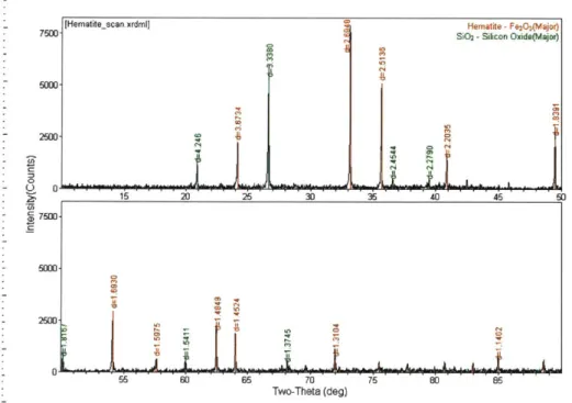
The laboratory powder X-ray diffractometer data turned out to be very accurate. The best example of success using the Search/Match function was with the hematite sample. The search returned only two possible matches: hematite and quartz. When plotted on top of the measured dataset, the two database spectra matched almost perfectly (Figure 7). Similarly, the spectrum for gypsum was a very good match. Gypsum was actually fourth in terms of FOM, but when comparing the match of gypsum to those of rancieite, brushite, and jamborite-the top three FOMs-it became obvious that gypsum was actually a better match. Although there were a number of peaks that did not show up in the measured data, the database spectrum of gypsum explained the most measured peaks.

The jarosite and anhydrite samples were slightly more complicated. When performing a SEARCH/MATCH on the jarosite [KFe, (SO4

),

(OH)6] sample, jarosite came up as the third

best FOM, behind straczekite [(Ca, K, Ba)2 V8020 -3H20] and berndtite [SnS2]. While the

database spectrum for jarosite did match up with a number of peaks in the data, there were still approximately 11 peaks that were not explained with by the jarosite dataset. In this

(24)

[Hematite scan.xrdml] Hematite -Fe2O3(Major)

30 -SiO2 -Siicon Oxide(Major)

NJn 10-15 20 25 30 35 40 45 0 0-20 253- 0 4 0. 55 60 65 70 Two-Theta (deg) 75 80 85 FMay. =27.2017 01:2p QdOIJAO)

Figure 7: PANalytical data for hematite. The black is the data collected on the PANalytical; the red peaks are the hematite d-spacing values from the database; and the green peaks are the quartz d-spacing values from the database.

0 0 Gyp um scan.xrdmil 10. Gypsum -Ca(SO4)(H20)2(10J 0%) 75- 252-15 20 25 30 35 4b 100 75-50. 45 55 S60 Two-Theta (deg) 65 70 75

F Ar127..207 On. 0:4p (iDJADE7)

Figure 8: PANalytical data for gypsum. The black is the data collected on the PANalytical, while the red peaks are the gypsum d-spacing values from the database. Although the intensity values do not match up, the peak positions are a good match.

751 251 0 U 75 I

(25)

(Jarosite scan.xrdmI] Jarosite -K(Fe3(SO4)2(OH)e)(100.0 3000-- 300- 2000-27 28 29 3) 31 32 33 34 35 36 37 38 39 40 41 30 0- 442000-2 43 440 4 47 48 3 34 3 37 39 2 5 40 551 57 56 59 60 61 62 63 64 65 66 67 68 69 70 71 Two-Theta (deg) Fdday. " 27. 2007 01:33p QD/JADE?)

[Jarositescan.xrdmi] Jarosite -K(Fe3(SO42(OH)e)(Minor)

300- Natrojarosie -NaFe3(SC4)2(OH)e(Majo) 1000-12 13 14 15 16 17 18 19 20 21 2 23 24 25 26 - 19 2b 21 22 23 2 27 28 29 3) 31 32 33 34 35 36 37 38 39 40 41 CC 3000-2000 4 42 2 43 4 45 47 0 4 49 51 32 533 5 36 3 839 540 55 15 3000- 2000- 1000-57 6b 59 so 61 62 63 64 65 66 67 68 69 70 71 Two-Theta (deg)

Frday. Ar" 27. 2007 01:" 2 OWDJDE)

Figure 9: PANalytical data for jarosite. The red peaks correspond to jarosite, and the green correspond to natrojarosite. The top plot shows the d-spacing database peaks of just jarosite, while the bottom plot shows how natrojarosite peaks match peaks that were not picked up by jarosite.

6 0 -'" 3"-0

(26)

low0-situation, a "paint peak" function was performed. The unidentified peaks were manually

"painted." Then JADE performed another SEARCH/MATCH, focusing on these painted peaks. The "paint peak" SEARCH/MATCH identified natrojarosite [NaFe3 (SO4)2 (OH),] as one of

the best matches. Jarosite and natrojarosite are both trigonal and chemically similar. Therefore, it seemed to make sense that the jarosite sample was a mixture of

jarosite

and natrojarosite. While this pair of minerals did not explain every peak of the dataset, it produced a good match (Figure 9).

Finally, the anhydrite sample was not pure. What made this dataset especially

challenging to analyze was that there was strong preferred orientation (Figure 10). The intense peak that corresponds to the 020 plane made every other peak incredibly small6_{. However, The}

SEARCH/MATCH function produced anhydrite as the second FOM. As with the gypsum

sample, anhydrite was the better match, because more of the peaks from the measured dataset

Fgr :d Cty Ot.e b p ts C rr. s Gys

7i

7

LJL

Li

752 3 44 46 46 57 AS 49 55 61

15 2 3553 3 4 55 66 17 6 5 1

TWO-TheMa(dog) TV00.heta (dog)

Figre 0: A~aytial ataforanhydrite. The black pattern is the measured pattern; the red peaks correspond to

the database d-spacings for anhydrite; and the green peaks correspond to the database d-spacings for gypsum. The left spectrum corresponds to large spacings (small angle), while the right spectrum corresponds to smaller

d-spacings (larger angle). They are separated because of the very strong peak at 29~ 25.50, which makes it difficult

to see the lower-intensity peaks at larger 20 values. Especially in the left image, it is evident that gypsum is present in the sample.

(27)

were explained by anhydrite than by ianthinite [(U0 2) .5(UO3) -10(H2O)], the top FOM.

However, of the 39 peaks in the measured dataset, 8 were not explained by anhydrite. Therefore, a "paint peak" function was again necessary, and revealed gypsum as the top FOM. This made sense, because gypsum (CaSO4 -2H20) is simply hydrated anhydrite (CaSO4). It is remarkable

how well the gypsum dataset filled in all of the peaks that were missing after matching the anhydrite database values with the dataset.

Table 4 lists the values determined for xoffset and zoffset-geometric corrections

discussed above-in addition to fluorescence lines and d-spacings. Since each sample was only run a handful of times, it is almost certain that not every orientation was captured by CXRDF. Therefore, it is understandable that fewer peaks were identified on CXRDF than are visible in the plots of data from the laboratory powder X-ray diffractometer. The real question is whether CXRDF is accurately identifying peaks that are representative of the minerals.

Table 4: CXRDF Data Mineral xoffset zoffset Fluorescence d-spacings

Anhydrite -90 5.5 Ca, S, P 1.52, 1.71, 2, 3.1, 3.49, 3.8

Gypsum -90 5.5 Ca, S, P 1.23, 1.25, 1.31, 1.45, 1.5, 1.6, 1.77, 1.88, 2.18, 2.5, 3.1, 3.75, 4.3

Hematite -80 6 Fe, Si _{1.49, 1.69, 1.82, 2.21, 2.51, 2.69, 3.34,}

3.72

Jarosite -120 7.5 Fe, Si, K, Ca 1.55, 2.25, 2.5, 2.8, 3.09, 3.1, 3.35

VI. Discussion

Comparing the CXRDF and the PANalytical data revealed a number of strengths and weaknesses of CXRDF. Looking generally at the data, it is evident that CXRDF was able to detect a number of d-spacings for each mineral. It was not always the case, however, that the detected d-spacings were among the most intense d-spacings found in powder X-ray diffraction experiments. It is not clear whether this is a downfall of the instrument's design or a downfall of

(28)

the software. In addition, although the range of the fluorescence data is somewhat limited, it is helpful and accurate. This important feature of the instrument may be key to the effectiveness of CXRDF.

The jarosite dataset was particularly helpful in revealing strengths and weaknesses of CXRDF. Two of the top three d-spacings for jarosite are 3.08A and 3.1 IA. The resolution of CXRDF is best at small d-spacings (large angles), with a d-spacing resolution of 0.04A at

2.088A [3]. Therefore, with the current detector, CXRDF would be unable to resolve two of the

top three d-spacings for jarosite. While it is possible to rotate the sample in such a way that

3.08A is illuminated in one run, and 3.11 A is illuminated in another, being able to illuminate only one d-spacing at a time would be more based on luck than skill. In addition, in the equally likely event that the sample is oriented such that diffraction occurred off of both sets of planes, it would be impossible to distinguish between the two. There are two possible solutions to this.

Figure 11: A plot of d-spacing vs. counts for jarosite. When compared to the laboratory powder XRD data, it is less obvious that there is natrojarosite present in the sample. However, database d-spacings for jarosite match the measured d-spacings fairly well. Finally, the close spacing of two of the three d-spacings for jarosite demonstrates the necessity of a high resolution detector.

(29)

First, the software could recognize that especially wide peaks (or arcs) may correspond to two separate d-spacings. Then, when performing a function such as findmin, it could acknowledge that an arc might be one, or it might be the merging of two separate d-spacings. However, this is only a temporary fix, as it inherently increases the uncertainty of the data. A real solution to the problem would be to utilize a detector that is capable of the resolution necessary to distinguish between two closely spaced d-spacings.

Another reason to improve the resolution of the detector is related to the fluorescence data. Some elements-such as Fe and Ca-fluoresce very brightly on the CXRDF data. As a result, d-spacings that are in the form of spots, as opposed to full arcs, can be "lost" in the fluorescence. Better resolution of this data may allow one to identify a spot within a fluorescence line, although this theory would need to be tested to be confirmed. A second possible solution would be to create a command that allows the software to remove fluorescence data. The difficulty in this is identifying which events that fall at the same energy and angle correspond to fluorescence, and which result from diffraction. One possibility is to take each individual value of 29 and find the average number of events that occur over a small energy range. The software could then subtract out the average number of events, perhaps revealing diffraction in areas that had a larger-than-average number of events at a given value of 20.

One strength of the instrument that was revealed by the jarosite data was the

incorporation of fluorescence data with diffraction data (Figure 12). When running afindmin command on the jarosite sample, it did not appear in the list of top 10 matches. However, when running findelem with Fe and K as the fluorescing elements, jarosite comes up 6 th out Of 10.

(30)

SM:O

-eT oi nd 7jar osi te. evt

Nsplthi tTheesamp

1 0

26 0dg)

Figure 12: A plot of Energy vs. 20 for jarosite. Fluorescence lines confirmn the presence of K and Fe, which are

expected in jarosite. There is also evidence of Si and Ca, which implies that there are impurities or a second mineral within the sample.

improve the effectiveness of the instrument7. In addition, in the hematite data from CXRDF, Si was identified as an element in the sample. Even if only a few quartz d-spacings were identified in the data, Si fluorescence could be a good hint that quartz was present, given how widespread quartz is, and that it is commonly associated with hematite.

7 However, it also raises the question of how impurities can affect the search. Whenfindelem was attempted with Fe

(31)

Looking more closely at the hematite sample, one can immediately recognize that

CXRDF was capable of definitively identifying hematite (Figure 13). This demonstrates that the instrument can identify one of the most important minerals in the discussion about whether there was once standing water on Mars. In addition, when comparing the data to the laboratory

powder XRD data, it becomes apparent that the additional arcs in the CXRDF data correspond to the d-spacings of quartz (Figure 14). On the one hand, this is very encouraging: CXRDF can

Figure 13: A plot of Energy vs. 20 for hematite. The yellow lines correspond to the top three d-spacings for the mineral hematite from the software's database. In addition, note the fluorescence line just below 2 keV, which corresponds to the fluorescence of Si.

(32)

Figure 14: A plot of d-spacing vs. counts for hematite. The plot shows a good match with hematite and quartz, with some peaks still unexplained by the top three d-spacings for the two minerals. The large hump in the data is a result of Fe fluorescence.

resolve d-spacings from at least two separate minerals simultaneously8. However, without knowing that quartz was present in the sample, it would be very difficult to determine what the

second mineral was. Although there are a number of peaks, it is unclear which belong to hematite and which belong to the second mineral. In addition, if it is obvious that there is a

8 This, of course, is dependent on the pair of minerals.

(33)

second mineral, is it possible that there is a third mineral? Then which d-spacings correspond to each of the three minerals? It is certainly not impossible to identify multiple phases using SM and the CXRDF data. However, the amount of time and effort that would need to be put into every sample becomes very daunting. It is possible that improving the data analysis software will help lessen this problem. If the software could recognize that a number of peaks were not explained by the spectrum for hematite-like the JADE software recognized when looking at the PANalytical data-then perhaps it could perform a second search to try and match the remaining peaks to an additional mineral. Improving the software would solve the problem without any changes to the instrument itself.

One can also confidently identify the presence of gypsum in the anhydrite data on CXRDF (Figure 15). While the CXRDF data for the anhydrite sample include one primary d-spacing for anhydrite, they actually contain two primary d-d-spacings for gypsum. This is slightly unnerving, since anhydrite has primary spacings that are in the middle of the range of d-spacings that can be detected by the instrument (3.49A, 2.85A, and 2.33A). The data therefore demonstrate the difficulty of using an unprepared sample. It would appear that in five separate runs, the sample was never oriented in such a way that two of the top three d-spacings for anhydrite were illuminated. In this sense, a direct comparison between powder diffraction and diffraction of an unmodified sample is very difficult to make. The intensities that have been identified with powder diffraction do not apply to a solid sample. Therefore, it would not be an

.9

appropriate analysis to look for only the top d-spacings determined from powder diffraction . One possible solution to this would be to alter thefindmin command. Rather than searching for

9 Here, the powder diffraction data that is being discussed relates to the database values that are used with the

findmin andfindelem commands, not the measured values from the PANalytical.

(34)

Figure 15: A plot of d-spacing vs. counts for anhydrite. Although the hump that results from the Ca fluorescence makes it difficult to see, the dataset does match with one of the top d-spacings for anhydrite (3.49A) and two of the top d-spacings for gypsum (3.07A and 4.28A).

minerals based on the hierarchy of the peaks identified with powder diffraction, perhaps the command should give weight to minerals that have the highest number of matched peaks, regardless of their relative intensities.

(35)

Figure 16: A plot of d-spacing vs. counts for gypsum. Only two of the top three d-spacings are visible because the

3rd d-spacing is too large to be detected by the instrument. Note that there are quite a few small d-spacings,

however, that could help to identify this sample as gypsum.

Identifying gypsum with this modified form offindmin would become much easier to do. When looking at the gypsum PANalytical data, the most prominent peak is at a d-spacing of

7.58A, which corresponds to a very small angle. Although CXRDF identified a number of

smaller d-spacings (Figure 16), it is not capable of picking up this d-spacing because of the Beryllium window coupled with the angle of the incoming rays. Recall that small angle

(36)

X-rays are low in energy. In addition, because they diffract at a small angle, they have to travel through a large portion of the Beryllium window. These low-energy X-rays that have to travel through a thicker portion of the Beryllium window are more likely to be absorbed, and are therefore not detected by the CCD.

To help solve this problem, Dr. Gendreau and his team are considering a new window geometry. The new set-up would have two windows that share an edge, oriented approximately perpendicular to the X-ray beam, in contrast to the current set-up of one straight window that forms an oblique angle with the beam (Figure 17). This would make the path through the Beryllium window shorter, while maintaining the structural integrity of the window. The new

Figure 17: Window geometries for CXRDF. The left figure is the current design, with the red arrows corresponding to X-rays, while the black horizontal line is the Beryllium window. The right figure is the proposed new geometry, with the two perpendicular black lines depicting the new window design, which is meant to shorten the path of the X-rays through the window.

angular shape of the window would mean the X-rays would most likely have to travel through a short distance of air before reaching the sample, depending on the shape of the sample.

However, calculations of the loss of signal in air versus the amount of absorption in Beryllium suggest that that the signal would still strengthen rather than weaken.

One could argue that it is not vital that the instrument be able to pick up large d-spacings. As discussed above, it may be possible to identify a mineral with many lesser-intense d-spacings.

(37)

However, this may not solve the problem. Clays, for example, have d-spacings larger than 10A, far beyond the instrument's current capabilities [13] [14]. If CXRDF is to identify clay minerals, it will actually need to improve its d-spacing range, not just its software.

It could also prove very important to improve the range of energies that can be detected

by CXRDF. There are a few elements just outside the range of detectable fluorescence that

might be very significant. On the low-energy end, it would be helpful to be able to detect K, Na, and Mg. The X-rays that result from fluorescence of these elements are currently not detected because they are absorbed by the Beryllium window. On the high-energy end, the highest-energy element that is detected is Ni, which fluoresces at 7.478

A.

However, Cu fluorescence occurs at 8.048 keV, while Zinc fluorescence occurs at 8.639 keV. These two elements are fairly common in minerals, and therefore it might be worthwhile to improve the maximum value of detectable fluorescence. With a different X-ray source, it might be possible to pick up higher energy fluorescence, revealing more about the sample.

VII. Conclusions

CXRDF will ultimately be very effective as a tool for definitive planetary mineral

identification. It successfully identified prominent d-spacings for the four minerals in discussion in this thesis, which suggests that it could help answer some questions about the geologic history of planetary bodies such as Mars. In addition, the fluorescence data proved to be very important, revealing clues about possible second phases in what were assumed to be pure samples. Finally, the fact that CXRDF successfully identified these minerals without any sample preparation means that it would be especially valuable for missions to other planets.

(38)

There are a few changes that are necessary for improving CXRDF's effectiveness. A

CCD that is capable of better resolution would greatly improve the instrument's ability to

distinguish between closely spaced d-spacings, and to identify d-spacings that are currently lost in very bright fluorescence lines. In addition, being able to identify larger d-spacings (smaller angle diffraction) and higher energy fluorescence would improve the instrument's ability to definitively identify minerals. However, the most important feature of the instrument that must be improved is the data analysis software. The instrument's design limits the range of d-spacings that can be detected. However, some of these limitations can be overcome with more advanced software. For instance, putting more weight on the number of d-spacing matches that occur, rather than the highest intensity peaks, may be a more appropriate way to search for a match between the obtained data and the database values. In addition, making sure thefindmin feature recognizes what d-spacings are simply beyond the range of the instrument would improve its effectiveness at correctly identifying minerals.

Finally, it may be beneficial for CXRDF to have the capability to powder a sample. Although the instrument is meant to be lightweight and to have the fewest number of moving parts possible, it may be important to be able to powder the surface of a rock. Currently, measurements are being taken only on the surface of the mineral. Therefore, in environments like that of Mars, CXRDF would likely be identifying a weathering rind that coats the true mineral underneath. While this rind itself may be significant to the geology, it will limit the instrument's ability to identify the overall composition of a given outcrop. In addition, as was evident in the anhydrite data, preferred orientation can make it very difficult to identify a mineral. Therefore, it may be useful to be able to powder a sample and thus take measurements on multiple orientations, as opposed to just one. This would not undermine CXRDF's overall

(39)

design-to be able to identify an unprepared sample-because it would still take measurements on solid samples when possible, and therefore be able to operate without any other moving parts. However, adding a grinding capability may add to its ability to definitively identify minerals with thick rinds or prominent cleavage planes.

It is important to keep in mind that the instrument that was evaluated in this thesis is only the second prototype of CXRDF. A third prototype has already been designed, and will soon be ready for testing. This third prototype has made the instrument smaller, as the goal is for the instrument to ultimately be portable and handheld. In addition, the new window design is being tested. This change is key, as it could mean that larger d-spacings will be detectable, along with lower-energy fluorescence.

VIII. Acknowledgements

I would like to acknowledge the designers of the instrument, Dr. Keith Gendreau and

Zaven Arzamounian. In addition, I would like to thank Carl Francis of the Mineralogical Museum at Harvard University and Dr. Jeffrey Post of the Mineral Sciences Division at the National Museum of Natural History for helping me to obtain samples of these minerals; Dr. Scott Speakman of MIT's Center for Materials Science and Engineering for his help in using the PANalytical Multipurpose X-ray Diffractometer; George Ricker Jr. and Peter Ford of MIT's Kavli Institute for Astrophysics & Space Research for their collaboration on this project; and finally my thesis advisor, Professor Sang-Heon Shim, for his help and guidance throughout this process.

(40)

IX. References

[1] ASU, undated, What is Emissivity?: <http://tes.asu.edu/MARSSURVEYOR/

MGSTES/TESemissivity.html> [follow "proceed to" links], (May 13, 2007). [2] Wenk, H. R. and Bulakh, A. (2004). "Mossbauer spectroscopy." Minerals: Their

Constitution and Origin. Cambridge: Cambridge University Press, 240-242.

[3] Gendreau, Keith et al, June 27, 2006, CCD Based Multi-Wavelength X-ray Diffractometer:

<http://esto.nasa.gov/conferences/ESTC2006/presentations/clpl.pdf>, (January 17,

2007).

[4] Blake, D. F. et al., March 13, 2007, Progress in the Development of CheMin: A Definitive

Mineralogy Instrument on the Mars Science Laboratory (MSL '09) Rover:

<http://www.lpi.usra.edu/meetings/lpsc2007/pdf/sess324.pdf> [16-17], (May 13, 2007).

[5] Bragg's Law: <http://www-outreach.phy.cam.ac.uk/camphy/xraydiffraction/

xraydiffraction7_1.htm>, (May 14, 2007).

[6] Amptek, November 5, 2002, X-ray Fluorescence Spectroscopy:

<http://www.amptek.com/xrf.html>, (May 14, 2007).

[7] Grotzinger, J. P. et al. (2005). "Stratigraphy and sedimentology of a dry to wet eolian

depositional system, Burns formation, Meridiani Planum, Mars." Earth Planet. Sci. Lett. 240, 11-72 (2005).

[8] Grotzinger, page 62.

[9] Knauth, L. P., Burt, D. M. and Wohletz, K. H. (2005). "Impact origin of sediments at the

Opportunity landing site on Mars." Nature 438, 1123-1128.

[10] Knauth, page 1123. [11] Knauth, page 1125.

(41)

[12] McCollom, T. M. & Hynek, B. M. (2005). "A volcanic environment for bedrock diagenesis at Meridiani Planum on Mars." Nature 438, 1129-1131.

[13] Tomita, K., Shiraki, K., and Kawano, M. (1998). "Crystal structure of dehydroxylated

2M1 sericite and its relationship with mixed-layer mica/smectite." Clay Science 10, 423-441.

[14] Heaney, P. J., Post J. E., and Evans, H. T. (1992). "The crystal structure of bannisterite."