An Analog VLSI Chip for Estimating the
Focus of Expansion
by
Ignacio Sean McQuirk
B. S., California Institute of Technology (1988) S. M., Massachusetts Institute of Technology (1991)
Submitted to the Department of Electrical Engineering and Computer Science in partial fulfillment of the requirements for the degree of
Doctor of Science at the
MASSACHUSETTS INSTITUTE OF TECHNOLOGY May 1996
@ Ignacio Sean McQuirk, 1996
The author hereby grants to MIT permission to reproduce and to distribute copies of this thesis document in whole or in part.
Signature of Author
-Department o ectrical Engineering and Computer Science June 6, 1996
Certified bn
ae- "un- .eLJ Professor of Electrical Engineering and Computer Science
Thesis Co-Supervisor Certified by B th ld K P H er o1/[1•iL .L .k. .. orn.~t.LL Professor of Electrical Engineering and Computer Science
Thesis Co-Supervisor Accepted by. .7ASSA C LIBRARIES
U
S
An Analog VLSI Chip for Estimating the Focus of
Expansion
by
Ignacio Sean McQuirk
Submitted to the Department of Electrical Engineering and Computer Science on June 6, 1996, in partial fulfillment of the
requirements for the degree of Doctor of Science
Abstract
For applications involving the control of moving vehicles, the recovery of relative motion between a camera and its environment is of high utility. This thesis describes the design and testing of a real-time analog VLSI chip which estimates the focus of expansion (FOE) from measured time-varying images. Our approach assumes a camera moving through a fixed world with translational velocity; the FOE is the projection of the translation vector onto the image plane. This location is the point towards which the camera is moving, and other points appear to be expanding outward from. By way of the camera imaging parameters, the location of the
FOE gives the direction of 3-D translation.
The algorithm we use for estimating the FOE minimizes the sum of squares of the differences at every pixel between the observed time variation of brightness and the predicted variation given the assumed position of the FOE. This minimization is not straightforward, because the relationship between the brightness derivatives depends on the unknown distance to the surface being imaged. However, image points where brightness is instantaneously constant play a critical role. Ideally, the FOE would be at the intersection of the tangents to the iso-brightness contours at these "stationary" points. In practice, brightness derivatives are hard to estimate accurately given that the image is quite noisy. Reliable results can nevertheless be obtained if the image contains many stationary points and the point is found that minimizes the sum of squares of the perpendicular distances from the tangents at the stationary points.
The FOE chip calculates the gradient of this least-squares minimization sum, and the es-timation is performed by closing a feedback loop around it. The chip has been implemented using an embedded CCD imager for image acquisition and a row-parallel processing scheme. A 64x64 version was fabricated in a 2pm CCD/BiCMOS process through MOSIS with a design goal of 200 mW of on-chip power, a top frame rate of 1000 frames/second, and a basic accuracy of 5%. A complete experimental system which estimates the FOE in real time using real motion and image scenes is demonstrated.
Thesis Co-Supervisor: Hae-Seung Lee
Title: Professor of Electrical Engineering and Computer Science Thesis Co-Supervisor: Berthold K. P. Horn
Biography
Ignacio Sean McQuirk was born on September 7, 1966 in San Pedro, California. Raised near Los Angeles, California, he attended the Mary Star of the Sea High School and graduated in 1984. He received the B.S. degree with honors from the California Institute of Technology, Pasadena, in 1988 and the S.M. degree from the Massachusetts Institute of Technology, Cam-bridge, in 1991, both in electrical engineering. His master's thesis was entitled "Direct Methods for Estimating the Focus of Expansion in Analog VLSI." He is a member of Sigma Xi, Tau Beta Pi, and a student member of the IEEE.
As a General Motors Scholar, Mr. McQuirk worked during the summers of 1986 and 1987 at Delco Electronics in Goleta, CA. The summer of 1986 was spent working on a digital control system design for the Hemispherical Resonator Gyroscope (HRG), a highly accurate gyro under development at the time. During the summer of 1987, he worked on an IEEE-488 I/O card circuit design destined for use in a variety of low cost guidance systems. Mr. McQuirk also spent the summer of 1988 working at AT&T Bell Laboratories in Whippany, NJ installing the Valid RealChip high-level digital hardware emulator as well as debugging the software integrating Valid RealChip into a functional system simulation and verification environment for high speed discrete digital designs.
Mr. McQuirk was a National Science Foundation Graduate Fellow from 1988 until 1991. He has also been an AT&T Bell Laboratories Cooperative Research Fellow from 1991-1996. Mr. McQuirk's current research interests center on analog circuit design applied to signal processing tasks.
Acknowledgments
This thesis describes research done at the Research Laboratory of Electronics, the Microsys-tems Technology Laboratories, and the Artificial Intelligence Laboratory of the Massachusetts Institute of Technology in collaboration with the MIT Vision Chip Project. Support for this work was provided by the National Science Foundation and the Advanced Projects Research Administration (grant numbers MIP-8814612 and MIP-9117724). Support for the author was provided in part by a National Science Foundation Graduate Fellowship as well as a Cooperative Research Fellowship from AT&T Bell Laboratories.I am deeply indebted to my thesis advisors, Professors Hae-Seung Lee and Berthold K.P. Horn, for all of their assistance in all of the various phases of this project. Professor John Wyatt also deserves many thanks for supervising the early stages of this work and for all of his efforts on behalf of the Vision Chip Group.
Chris Umminger and Steven Decker have been of great help, providing useful comments and advice over the years as this research progressed. Craig Keast, Mikko Hakkarainen, and Lisa Dron deserve kudos for the technical assistance they gave in the CCD aspects of the design of the FOE chip. Thanks also go to Bob Armstrong and Ricardo Telichevesky for giving invaluable assistance in the design and testing of the FOE system.
Amelia Shen, Chavela Carr, and Jennifer Lloyd have provided me at various times with more emotional support then they perhaps realize, and for that I am deeply grateful.
Finally, thanks to my parents and the rest of my family who have been so supportive of my education. I deeply appreciate all that they have done for me.
Si es real la luz blanca
de esta ldmpara, real
la mano que escribe, ison reales
los ojos quie miran lo escrito?
De una palabra a la otra
lo que digo se desvanece.
Yo sd que estoy vivo
entre dos parentesis.
Contents
Abstract 3 Biography 5 Acknowledgments 7 List of Figures 14 List of Tables 21 1 Introduction 232 Direct Methods for Estimating the Focus of Expansion 27
2.1 The Brightness Change Constraint Equation . . . 27
2.2 Algorithms Based on the Brightness Change Constraint Equation . . . 30
2.2.1 Rotation and Translation When Depth is Known or Structured . . . 30
2.2.2 Translation: The Eigenvalue/Eigenvector Solution . . . 33
2.2.3 Translation: The Linear Solution . . . 34
2.2.4 Translation: Minimizing Z2 . . . 35
2.2.5 Translation: Minimizing the Number of Negative Depth Values . . . 37
2.2.6 Translation: Algorithms Based on the Distribution of Negative Depth Values . . . 38
2.2.7 Translation: Solutions Which Favor Smoothness of Depth . . . 41
2.3 Algorithmic Simulations ... 42
2.3.1 Synthetic Image Generation ... 42
2.3.2 Simulation Results ... 44
3 The FOE Chip System Architecture and Circuit Design 47 3.1 Potential Approaches ... .. ... ... ... ... ... .. ... ... ... .47
3.2 Richardson's Iterative Method . .. .. . . .. . . . ... .49
3.4 Architecture Simulation ... 3.5 Circuit Structures ...
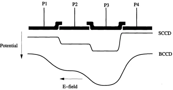
3.5.1 Charge Coupled Device Fundamentals . . . . 3.5.1.1 The MOS Capacitor . . . . 3.5.1.2 The Delta-Depletion Approximation . . . 3.5.1.3 The Potential Well Analogy . . . .
3.5.1.4 The Surface Channel CCD . . . . 3.5.1.5 Charge Storage and Dark Current . . . .
3.5.1.6 CCDs as Analog Shift Registers . . . . . 3.5.1.7 Transfer Inefficiency . . . . 3.5.1.8 Imaging ...
3.5.1.9 Charge Input ... 3.5.1.10 Charge Output ...
3.5.1.11 The Buried Channel CCD . . . . 3.5.2 The Interline CCD Imager with Storage . . . . 3.5.3 The CMOS Processing Array ...
3.5.3.1 Estimating the Brightness Gradients . . . 3.5.3.2 The Cutoff Weighting Function . . . . 3.5.3.3 Getting the Brightness Gradient Squared 3.5.3.4 The Multiplier Core . . . . 3.5.4 The Position Encoder ...
4 The FOE Test System
4.1 The Motion Problem ...
4.2 The Optical/Mechanical Subsystem . . . .
4.2.1 The Flexible Image Carrier . . . . 4.2.2 The DC Motor System . . . .. 4.2.3 The Distal Interface ...
4.2.4 The Proximal Interface ... 4.3 The Electrical Subsystem ...
4.3.1 Clocking .... ... . .. . ...
4.3.2 The Feedback Control Processor . . . .
4.3.3 Interfacing the Chip to the Test System 4.3.3.1 The ADC Interfaces... 4.3.3.2 The DAC Interfaces ...
. . . .125
CONTENTS
... ... . . . . .• . . . . . . . . . . . . . . . . . . ..1 . . . . . . . . . . . . . ... ... ... . o. . . . . . . . . . . ... ., . . . . . . . . . Magnitude ., . .• .., . ,... 103 .103 S104 104 .107 108 110 .113 .115 .118 .119 .120 .122 ... . . . . . . . . . . . . . . . . . . . . . . . . . . . . . . . . . . . . . . . . . . . . . ... ... ... . . . . . . . . . . . . . . . . . . . . . . . . . . . . . . . . . . . . . . . . . . . . . ... ... 4.3.4 Later Enhancements ...CONTENTS
5 The 5.1 FOE Basic 5.1.1Chip/Test System Results Functionality ...
I/O Results from the CMOS Processing Array ...
129
... 129
... 129
5.1.1.1 The Absolute Value and the Cutoff Weighting Function . . . 129
5.1.1.2 Estimating the Gradient Magnitude .
5.1.1.3 The Multiplier Core . . . . 5.1.1.4 The Position Encoder . . . . 5.1.2 Basic CCD results ...
5.1.2.1 Charge Input and Output . . . . 5.1.2.2 Transfer Inefficiency . . . . 5.1.2.3 Dark Current . . . . 5.1.2.4 Optical Responsivity . . . .
5.1.3 Electrical Input and Electrical Output . . . . .
5.2 Imaging Results: Raw Image Data . . . .
5.2.1 The Target Image ...
5.2.2 Optical/Mechanical Preliminaries . . . . 5.2.3 Camera Calibration using Rotation . . . . 5.2.4 Imaging Results: Finding the FOE . . . . 5.2.4.1 Biases in the Solution . . . . 5.3 Processed Data Results: Finding the FOE . . . .
131 133 135 135 135 142 143 144 146 150 150 153 155 158 159 166 6 Conclusions 6.1 Summary 177 . . . .177
6.2 Improvements and Future Work ... . . . .177
List of Figures
1-1 Illustration of the passive navigation scenario . . . . . 25
2-1 Viewer-centered coordinate system and perspective projection . . . . . 28
2-2 Definition of the location of the focus of expansion . . . 30
2-3 Permissible bands of s on the unit sphere . . . 34
2-4 The great circle which fits the distribution of directions of s vector for the set of stationary points ... 35
2-5 Determination of permissible and forbidden regions for directions of Er . . . . . 39
2-6 The map of probabilities that the depth-is-positive constraint is violated .... . 40
2-7 Pixel cube used in estimating the the three partial derivatives of image brightness from an image pair. ... 43
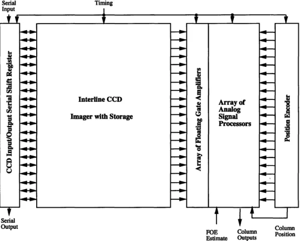
3-1 Block diagram of the system architecture of the FOE chip . . . . . 51
3-2 Simulated FOE system transient on synthetic image data with (x0, Yo) = (22.5,42.5). Loop gain hAmax is less than 1... 53
3-3 Simulated FOE system transient on synthetic image data with (x0, yo) = (22.5,42.5). Loop gain hAma, - 1 . ... 53
3-4 Simulated FOE system transient on synthetic image data with (x0, Yo) = (22.5,42.5). Loop gain satisfies: 1 < hAmax _ 2... 54
3-5 Simulated FOE system transient on synthetic image data with (x0, yo) = (22.5,42.5). Loop gain hAmax Z 1. Saturating multipliers and sums are modeled . . . . . 54
3-6 Photograph of the fabricated FOE chip with the various components indicated. . 56 3-7 An M OS Capacitor. ... 57
3-8 Energy band diagrams and charge distributions for the MOS capacitor . . . . . 58
3-9 The potential into the semiconductor for a deep-depletion MOS capacitor with 0, 1/4, 1/2, 3/4, and full charge . . . . . 60
3-10 The potential well analogy. ... 61
3-11 Diagrammatic representation of a typical surface-channel CCD . . . . . 61
LIST OF FIGURES
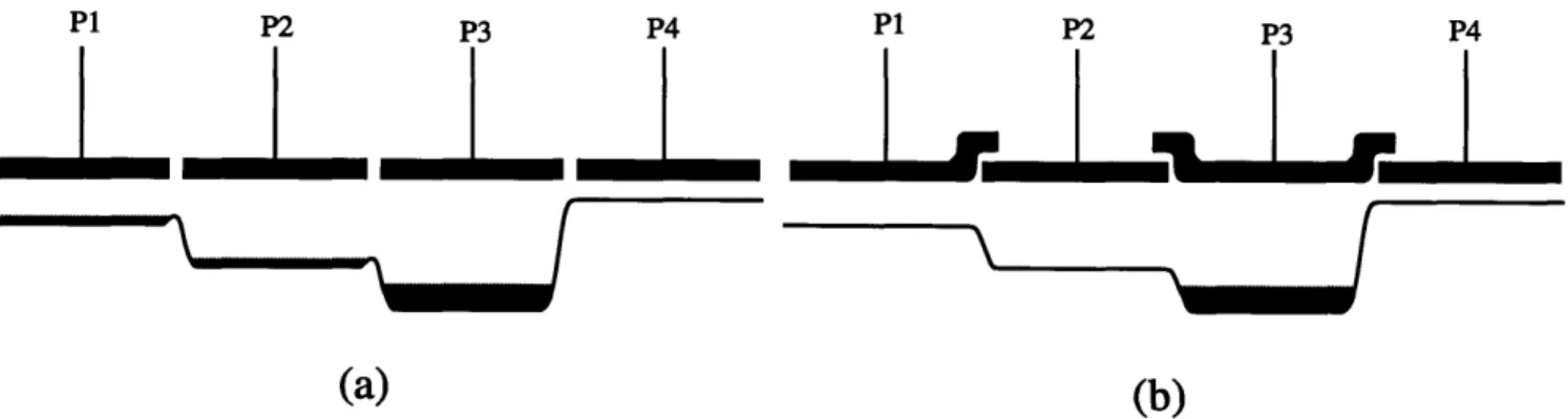
3-13 (a) Potential "bumps" caused by gate separation leading to transfer inefficiency.
(b) Overlapping gate structure alleviating potential "bumps" . . . . . 64
3-14 Typical optical CCD responsivity. . . . 66
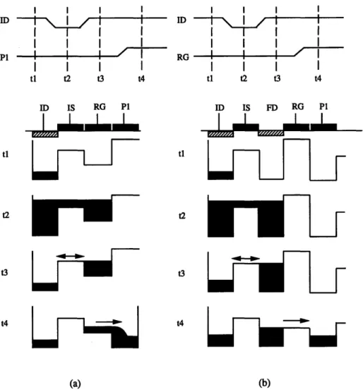
3-15 Input structures, clocking waveforms, surface potentials, and signal charge, for (a) the standard fill-and-spill approach and (b) for the split-gate fill-and-spill technique . . . 67
3-16 Potentials and charge locations during shifting and sensing for (a) the floating diffusion output structure and (b) the floating gate output structure . . . . . 68
3-17 Required clock waveforms for output using (a) the floating diffusion output struc-ture and (b) the floating gate output strucstruc-ture . . . . . 69
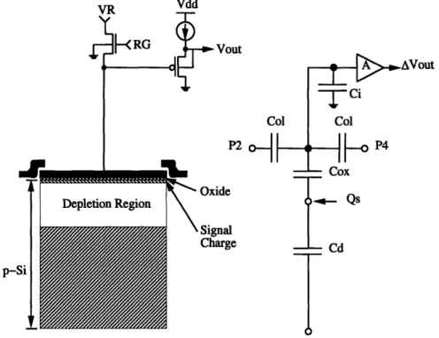
3-18 Lumped circuit model for the floating gate output structure in a surface channel CCD. . . . ... . .. 70
3-19 Diagrammatic representation of a typical buried-channel CCD, including input and output structures ... 72
3-20 Energy band diagram for buried channel COD with (a) no charge, and (b) with charge .. . . . 73
3-21 The potential into the semiconductor for a buried channel CCD . . . . . 73
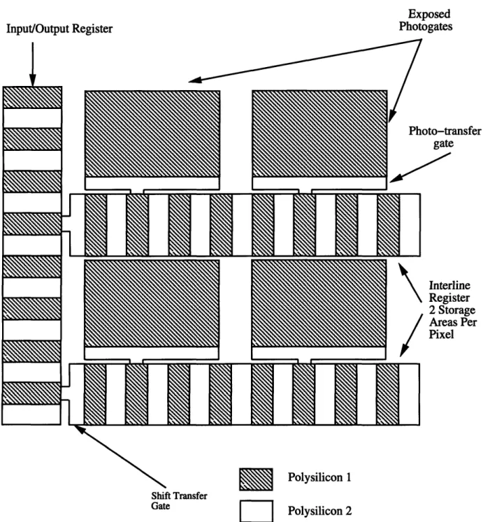
3-22 Burying the channel leads to smoother fringing fields enhancing transfer efficiency. 74 3-23 Schematic representation of the interline CCD imager on the FOE chip . . . . . . 75
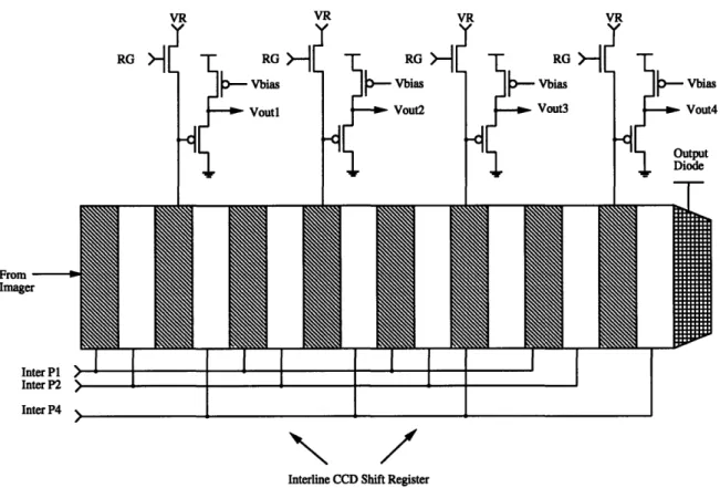
3-24 Estimating the image brightness gradients requires four floating gate outputs in a row . . . . . 77
3-25 Lumped circuit model for the floating gate output structure in a buried channel CCD . . . . . 77
3-26 Block diagram indicating the structure of analog row processor in the cMOS processing array. ... ... 79
3-27 A simple source coupled pair is used to transduce voltage signals from the floating gate outputs to current signals for gradient estimation . . . . . 81
3-28 Normalized input differential voltage to output differential current transfer char-acteristic of the source-coupled pair . . . . . 81
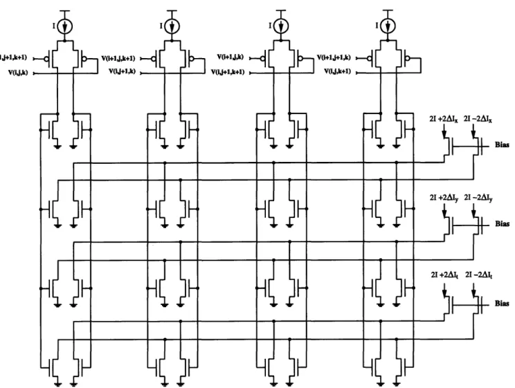
3-29 Using transconductors and mirrors to generate the first centered difference ap-proximations to the image gradients ... 83
3-30 Block diagram representation of the Cutoff Weighting Function . . . . . 83
3-31 Circuit implementation of the Cutoff Weighting Function . . . . . 84
3-32 One stage of the masking shift register . . . 84
3-33 Applying the result of the Cutoff Weighting Function to the brightness gradient. 87 3-34 A simple three transistor current mode MOS quadratic circuit with its bias tree. 87 3-35 Full circuit implementation for finding the brightness gradient squared magnitude. 89 3-36 Four-quadrant bipolar Gilbert multiplier . . . . . 90
LIST OF FIGURES
3-37 A simple MOS version of the Gilbert multiplier . . . 91
3-38 Normalized input differential voltage to output differential current transfer char-acteristic of the MOS multiplier ... 92
3-39 The first layer of multipliers with output mirroring . . . 95
3-40 The second layer of multipliers with triode-based I/V converter . . . 95
3-41 Mesh plot of the normalized DC transfer curve of the analog processor found by driving E. (C) maximally ... 96
3-42 Family of curves obtained by slicing the surface in the
C
direction . . . . . 973-43 Family of curves obtained by slicing the surface in the i direction . . . . . 97
3-44 Circuit diagram of the position encoder . . . . . 99
3-45 The simple two-stage operational amplifier used in the position encoder . . . . . 100
3-46 SPICE gain response of operational amplifier used in multiplexed position encoder. CL = 10pF . . . .. .. . .. . . . .. . . .. . . . .100
3-47 SPICE phase response of operational amplifier used in multiplexed position en-coder. CL = 10pF . ... 101
3-48 SPICE step response of operational amplifier used in multiplexed position encoder. CL = 10pF . .. . .. . . . . .. . .. . . . .. . . .. . . . .101
4-1 A high level view of the basic test setup, showing the two major subsystems: optical/mechanical, and electrical . . . . . 104
4-2 a). Light within the critical angle <p given can be transmitted down an optic fiber using total internal reflection. b). The principle of image transmission by an image guide. c.) Flexible fiber-optic carrier used in remote visual inspection. .105 4-3 The physical structure of the mechanical and optical system . . . . . 107
4-4 The distal mount, allowing placement of the FOE anywhere in the image plane. .109 4-5 The distal clamp for attaching carrier to the distal mount . . . . . 109
4-6 Optical interface to the proximal mount . . . . . 111
4-7 The proximal end, showing attachment to the FOE board . . . . . 112
4-8 Block diagram and floorplan of the FOE system board . . . . . 114
4-9 Block diagram of the pattern generator for generating all clock waveforms on the FOE board . . . ... 116
4-10 Sample design for a clock driver with adjustable levels and rise/fall times... . 116
4-11 DSP system for implementing discrete time feedback loop . . . . . 120
4-12 Board interface for the error output channels from the FOE chip . . . . . 121
4-13 Board interface for the absolute value output channel from the FOE chip .... . 122
4-14 Board interface for the quadratic output channel from the FOE chip. . . . 123
4-15 Monotonic voltage output DACs are used to generate the position voltages (Vxo, Vyo) for the FOE location ... 124
LIST OF FIGURES
4-17 Output circuit for one of the 8 CCD I/O channels . . . 127
4-18 Circuit schematic for the muxing daughter board . . . 127
4-19 Simple water-based cooling system for the FOE chip . . . 128
5-1 Absolute value characteristic measured from the test cell provided on the FOE chip . . . .130
5-2 The cutoff weighting function characteristic, large scale. Et is driven maximally and the lines represent the 50% switching points . . . 131
5-3 The cutoff weighting function characteristic, small scale . . . . . 132
5-4 Measured quadratic circuit characteristic with E, driven maximally . . . . . 132
5-5 The family of curves for the x-channel output current of the test cell parameter-ized by x - x0 . ... 134
5-6 The family of curves for the x-channel output current of the test cell
parameter-ized by E~. . . .. . . . .. . . . ... 134
5-7 Scope trace of y-channel output with Ey maximally driven . . . . . 136
5-8 Scope photograph showing the settling time of the test cell. The output circuit is the same as on the main array. The traces in order from top to bottom are Oreset, Olatch, e, and
W
... 1365-9 Scope waveform showing operation of the position encoder over an image frame. 137 5-10 Magnified scope waveform showing operation of the position encoder . . . . . 137
5-11 Source follower characteristic from pre-charge voltage to output . . . . . 139
5-12 Nonlinearity of the source follower characteristic . . . . . 140
5-13 Input to output characteristic of the I/O shift register . . . . . 141
5-14 Illustration of the measurement of CCD transfer inefficiency using the step re-sponse of a shift register...142
5-15 Illustration of the measurement of dark current . . . . . 145
5-16 Setup for measuring the quantum efficiency of the imager on the FOE chip. . . .145
5-17 Plot of the measured output signal as a function of incident light power . . . . . 146
5-18 Setup for introducing test patterns into the FOE chip . . . . . 147
5-19 Measured absolute value characteristic for four processors in the main array under Et excitation . ... 148
5-20 Weighting function characteristic measured from a processor in the main array. .149 5-21 Family of curves obtained for the y-channel from a processor in the main array under E. excitation ... 151
5-22 Family of curves obtained for the x-channel from the bottom processor in the main array under E. excitation ... 152
5-23 Illustration of target scene used in the lab . . . . . 153
LIST OF FIGURES
5-25 Sample motion sequence. The settings of the distal mount are 0 = -90 and
S= 13.50 placing the FOE in the upper left hand corner as indicated by the cross. 156
5-26 Target scene with 0 = 0 and
0
= 50. Detected features are indicated by "x"s while the center of the image target is indicated by "*" . . . . . .1585-27 Example of the algorithm in action. The settings of the distal mount are 0 = -18' and q = -18' placing the FOE in the lower left hand corner as indicated by the x. The track of the motor system is visible in the upper left hand corner. 160 5-28 Results of raw image data taken from imager on FOE chip .. . . . .161 5-29 Geometry used to consider sensitivity of the stationary point weighting to
devi-ations in the solution . ... 162 5-30 Geometry for considering the effects of the cutoff weighting function .. . . . . .164 5-31 Simple geometry of a band about a stationary point .. . . . .165 5-32 Least squares solution given by the center and endpoints of a band about a
stationary point . . . .. . . . . .. . . . .. 166 5-33 Illustration of the situation when the FOE is near the image boundary.
Con-straints from features that would normally counteract the stationary band at-traction are absent due to the finite image size .. . . . .167 5-34 Measured offsets for the entire column of processors for the absolute value channel
and the gradient magnitude channel .. . . . .167 5-35 Measured offsets for the entire column of processors for the absolute value channel
and the gradient magnitude channel .. . . . .168 5-36 Mesh plot of |Et as calculated by the FOE chip with frontal motion .. . . . . .169 5-37 The image of the
lEt!
channel during frontal motion is shown on the left, andon the right is the binary image representing the result of applying the cutoff weighting function . ... ... ... ... ... 169 5-38 Lumped circuit model for the set of four floating gate amplifiers including the
effects of the layout error ... 170 5-39 The image of the gradient magnitude channel during frontal motion is shown on
the left, and on the right is the binary image representing the result of applying the gradient thresholding ... 171 5-40 Simple op-amp circuit for correcting the sign error on the FOE chip . . . . . . .172 5-41 Mesh plot of the x error channel output. Motion is frontal, and the FOE estimate
is at the im age origin . ... 173 5-42 Mesh plot of the y error channel output. Motion is frontal, and the FOE estimate
is at the im age origin . ... 173 5-43 Transient response of the FOE chip and feedback loop. Motion was frontal, and
20
LIST OF FIGURES
5-44 Example of the algorithm in action using the FOE chip in a simple constant gain feedback loop ... ... .. 174 5-45 Comparison of distorted FOE locations (o's) with the results of algorithmic
pro-cessing of raw image data (x's) and the estimates provide by the FOE chip closed in the feedback loop (+'s) . ... 175
List of Tables
4-1 Typical image carrier parameters.. . .. .. . . . . .. 106
4-2 Specifications of the Klinger motor system used in the experimental setup for testing the FOE chip ... 108
5-1 Table of device parameters for the floating gate amplifiers . . . 138
5-2 Summary of CCD performance parameters . . . . . 147
5-3 Summary of FOE chip camera calibration parameters . . . 159
Introduction
Some attention has recently been given to the potential use of custom analog VLSI chips for early vision processing problems such as optical flow [1, 2], smoothing and segmentation [3, 4, 5, 6, 7, 8] orientation [9, 10], depth from stereo [11, 12], edge detection [13, 14] and alignment [15, 16]. The key features of early vision tasks such as these are that they involve performing simple, low-accuracy operations at each pixel in an image or pair of images, typically resulting in a low-level description of a scene useful for higher level vision. This type of processing is well suited to implementation in analog VLSI, often resulting in compact, high speed, and low power solutions. These chips exploit the inherent parallelism of the computation along with the close coupling of the processing circuitry with the image sensor. This thesis details the application of this approach of focal plane processing to the early vision task of passive navigation.An important goal of motion vision is to estimate the 3-D motion of a camera in an envi-ronment based on the resulting time-varying image sequence. Traditionally, there have been two basic approaches to this problem: feature based methods and motion field based methods. In feature based methods, an estimate of motion and scene structure is found by establishing the correspondence of prominent features such as edges, lines, etc., in an image sequence [17, 13]. In motion field based methods, the apparent velocity of points in the image, the optical flow [18], is used to first approximate the projection of the three dimensional motion vectors into the image plane, the motion field. The optical flow is then used to estimate the camera motion and scene depth [19]. Both the correspondence problem and optical flow calculation have proven to be difficult in terms of reliability and implementation. We therefore look to methods which directly utilize image brightness information to recover motion [20, 21, 22, 23]. These methods lead to computations in the image domain rather than symbolic or sequential computations.
The introduction of the focus of expansion (FOE) for the case of pure translation simplifies the general motion problem significantly. The FOE is the intersection of the translation vector of the camera with the image plane. This is the image point towards which the camera is moving, as shown in Figure 1-1. If the camera velocity has a positive component along the optic axis,
CHAPTER 1. INTRODUCTION
features will appear to be moving away from the FOE and expanding, with those close to the FOE moving slowly and those further away moving more rapidly. Through knowledge of the camera parameters, the FOE gives the direction of camera translation. Once the FOE has been determined, we can estimate distances to points in the scene being imaged. While there is an ambiguity in scale, it is possible to calculate the ratio of distance to speed. This allows one to estimate the time-to-impact between the camera and objects in the scene. Applications for such a device include the control of moving vehicles, systems warning of imminent collision, obstacle avoidance in mobile robotics, and aids for the blind.
This thesis investigates the design and implementation of a chip in analog VLSI for estimation of the focus of expansion produced by camera motion. The goal of the project is to demonstrate the chip functioning in a complete motion vision system operating in real time using real motion with real image scenes. Consequently, the thesis is divided into three basic parts: a review of the algorithm chosen for implementation along with its theoretical basis, a description of the
FOE chip architecture and its circuit design, and the test system and experimental setup devised to accomplish our goal.
The thesis begins in Chapter 2 by describing the algorithmic foundations for the FOE chip. The brightness change constraint equation, which forms the basis for our differential approach to the motion vision problem, is derived, allowing the formulation of a variety of low-level approaches suitable for implementation. The conclusions provided by extensive simulation of these algorithms along with a knowledge of what is feasible in analog VLSI allows us to pick one of these algorithms for implementation. Chapter 3 provides a detailed description of the structure and operation of the final architecture settled upon along with its associated circuit components. Chapter 4 describes the test system and experimental setup designed to support the chip, as well as the requirements resulting from the necessity of using real data from real motion in real time. Chapter 5 presents the test results of the FOE chip, from the circuit level to the system level to the algorithmic level, confirming its operation and characterizing its performance. Finally, the work is summarized and concluding comments made in Chapter 6.
xo I
Apparent Motion
of Image Points
Optic Axis
Camera
/
Direction of Motion
Time-to-Impact =
Depth
Velocity
FIGURE 1-1: Illustration of the passive navigation scenario, showing the definition of the focus of expansion as the intersection of the camera velocity vector with the image plane.
Foc. o.f ,
2
Direct Methods for Estimating the
Focus of Expansion
2.1
The Brightness Change Constraint Equation
The brightness change constraint equation forms the foundation of the various direct algo-rithms for rigid body motion vision [23, 21, 24] that we have explored for potential implemen-tation in analog VLSI. It is derived from the following three basic assumptions:
* A pin-hole model of image formation. * Rigid body motion in a fixed environment.
* Instantaneously constant scene brightness.
Following [21, 24, 19], we use a viewer based coordinate system with a pin-hole model of image formation as depicted in Figure 2-1. A world point
R (X, Y, Z)T (2.1)
is mapped to an image point
r
(x, y,
f)T
(2.2)
using a ray passing through the center of projection, which is placed at the origin of the coordinate system. The image plane Z =
f,
wheref
is termed the principal distance, is positioned in front of the center of projection. The optic axis is the perpendicular from the center of projection to the image plane and is parallel to the Z-axis. The x- and y-axes of the image plane are parallel to the X- and Y- axes and emanate from the principal point (0, 0,f)
in the image plane. The world point R and the image point r are related by projection:r
R
CHAPTER 2. DIRECT METHODS FOR ESTIMATING THE Focus OF EXPANSION
Z
FIGURE 2-1: Viewer-centered coordinate system and perspective projection.
which is the perspective projection equation [25]. To find the motion of image points given the motion of world points, we differentiate Equation 2.3 using the chain rule:
re =
~(R
--)Rt - (Rt --)R)(24
rt = (R •.)2
((ZR
-(Rt
•)R) (2.4)where we have defined
dR dX dY dZ )T
R
dt
dt dt ' dt ' dt (2.5)rt = d dt , dOT (2.6)
We can rewrite Equation 2.4 as
r = ( x (Rt x R)) _ x (Rt x r)(2.7)
rt (R .) 2 = R (2.7)
Next, we introduce the constraint implied by having the camera move relative to a fixed envi-ronment with constant translational velocity t = (t., ty, t)T and constant rotational velocity w = (w, w,, w,)T. The resulting motion of a world point R relative to the camera satisfies:
Rt = -t - (w x R) = -t - (w x r)
(R
(2.8)Clearly, this constraint is valid only for instantaneous motion. Combining this with Equa-tion 2.7, we arrive at a parameterizaEqua-tion of the moEqua-tion field rt:
(r(r
rt = -Z x r x (2.9)
A common method to relate the motion field rt to the measured image brightness E(x, y, t)
is to do so through the constant brightness assumption [23]. We assume that the brightness of a surface patch remains instantaneously constant as the camera moves. This implies:
dE
dE
= Et + Er - r = 0 (2.10)dt
R ,Y,Z)
2.1. THE BRIGHTNESS CHANGE CONSTRAINT EQUATION
OE
OE
TEEt =- 9E , Er = (Ez, E,0)T = OE O ' O (2.11) In practice, the constant brightness assumption is valid for a large class of image sequences [18]. Combining Equation 2.9 and Equation 2.10, we have:
Et-Er -
rx
(fR
0
(2.12)
To simplify this expression, we can define the new image quantities s and v as follows:
s (Er x )x r, v-rxs
(2.13)
Through the use of some vector identities, we find:
Er - (x (rx t)) = ((Er x Z) x r) -t (2.14)
Er .( x (rx ×(x w))) = - v.w - (2.15)
Combining these results with Equation 2.12, we have:
v*w s.t
Et
+
+
= 0 (2.16)f
R
Z
This is known as the brightness change constraint equation.
Now, in order to investigate the case of pure translation, we set w = 0: s't
Et + s = 0 (2.17)
This equation remains the same if we scale both the depth Z and translational velocity vector t by the same scale factor. This ambiguity is referred to as the scale-factor ambiguity. Defining the FOE:
ro = (xo, Y0o, f) (2.18)
as the intersection of the translational velocity vector t with the image plane as in Figure 2-2, the following relation results:
ft
r -= (2.19)
Again using vector identities, we can note that
s -ro = ((Er x i) x r) - ro
= (Er - r)(. -ro) - ( - r)(Er -ro)
=
fEr
- (r- ro) (2.20)Combining Equations 2.17, 2.19 and 2.20, we derive our final result for the case of pure trans-lation:
CHAPTER 2. DIRECT METHODS FOR ESTIMATING THE Focus OF EXPANSION
Z
FIGURE 2-2: Definition of FOE location as intersection of velocity vector t with the image plane.
which is the brightness change constraint equation for the case of pure translation. This can also be expressed using components as
rEt
+ (x
-
xo)Ex
+ (y
-
yo)E,
=
0
(2.22)
7 - Z(X, y)/t.
The time to impact r is the ratio of the depth Z to the velocity along the optic axis tz. This is a measure of the time until the plane parallel to the image plane and passing through the center of projection intersects the corresponding world point. The time-to-collision of the camera is the time-to-impact at the focus of expansion.
2.2
Algorithms Based on the Brightness Change Constraint
Equation
Having derived the brightness change contraint equation, we can now turn to algorithms utilizing this differential constraint with the goal of constructing a dedicated analog VLSI chip to estimate camera motion through the FOE .
2.2.1
Rotation and Translation When Depth is Known or Structured
Finding both rotation and translation when scene structure is also unknown is difficult chiefly due to the dependence of Z on x and y. For example, if we have n x n brightness gra-dient measurements, then we have n2 constraints provided by the brightness change constraint equation but 6 more unknowns than that, producing an underconstrained system. If we assume that somehow we are provided with the depth map Z(x, y), then the problem becomes over-constrained with six unknowns and n2 constraints. Hence, we utilize least-square minimization
t )
1
y, t z)2.2. ALGORITHMS BASED ON THE BRIGHTNESS CHANGE CONSTRAINT EQUATION
to find a solution. We can minimize with respect to w and t an integral over the image of the squared error of the constraint equation:
mi n/
f / ( E v c .t- ) 2
i
(Et
+ v
f
+
dJdy
(2.23)
Differentiating and setting the result equal to zero to find the extrema yields a closed form solution:
ft T
dTdy
(fI
dxdy
dxdy
=[
]
(2.24)
dzdy J 2)dxdy
dxdy
Alternatively, if we know that the scene geometry is one of a parameterized family of surfaces, then we can also have an over-constrained system. For example, consider the simple case of a scene consisting of a single plane of unknown depth. The equation for a plane is:
R - n = 1 (2.25)
where n is a normal to the plane. Imposing the perspective projection equation (2.3) implies:
Z- f (2.26)
r-n
Combining this with the brightness change constraint equation, we have:
fEt + v - w + (r - n)(s - t) = 0 (2.27) Now, we have nine unknowns (the components of t, w, and n) and can solve using least squares methods. Again, we can minimize the sum of the squared error over the image:
( )2
min
(Et
+ v-w +
(r-
n)(s. t))2dxdy
(2.28) W,t,n 11,Differentiating this expression and setting the result equal to zero gives:
fI
(fEt+
v -w+(r. n)(s . t))vdxdy = 0 J (r.n)(fEt+v-w+(r.n)(s.t))sdxdy = 0Jj(s-t)(fEt+v-w
+
(r. n)(s-t))rdxdy = 0 (2.29)Even though these equations are nonlinear, there are iterative methods for their solution and, in fact, a closed form solution using eigenvalue/eigenvector analysis [26].
Another approach to simplifying the situation imposed by the local variation of the depth map Z is to remove the translational component entirely. When we only have rotation, then the brightness change constraint equation becomes especially simple:
CHAPTER 2. DIRECT METHODS FOR ESTIMATING THE FOCUS OF EXPANSION
This is always an over-constrained problem with three unknowns and n2 constraints, one for
every picture cell. We can minimize the square of the error of this equation:
(V*W2
minJ (Et + -
) dxdy
(2.31)
w
f
to find the solution
(vvT)
dxdy] w
=-f
(vEt) dxdy
(2.32)
which is clearly just a special case of Equation 2.24.
To examine when this least-squares method for recovering rotational velocity becomes ill-conditioned, an analysis was performed in [21] assuming a uniform distribution of the allowed directions of v which demonstrated that the L2 condition number of the matrix in the left hand side of Equation 2.32 increases as the extent of the field of view (Fov) decreases. The FOV is the cone of r directions defined by the principal distance
f
and finite extent of the image plane. With this analysis, the condition number reaches a minimum at a half-angle 0, = 57.420. In general, the third component of w, the rotation about the optic axis, is not recovered as accurately as the other two. The relative error between the third component and the other two varies inversely with the Fov [21].Obviously, the more difficult situation due to the local variation of Z, and hence the more interesting one, is when we have some sort of translational motion. For simplicity, we will from now on eliminate the rotational component. Again, known scene geometry can greatly reduce the difficulty of the problem. As an example of a plain scene geometry, we can assume the presence of a plane perpendicular to the optic axis at a distance Zo. In this case the solution becomes:
sS) dxdy] t' = - (sEt) dxdy (2.33)
t
t'-
-
(2.34)
-Zo
The third component of t' is the now constant time to impact T. Notice the similarity to the
solution for the case of pure rotation in Equation 2.32. The observations we noted for pure rotation also hold in this case. The condition number of the matrix in Equation 2.33 decreases with increasing FOV, reaching a minimum at half-angle 0, = 54.740, and the accuracy with which we recover the third component is always less than the other two and varies inversely with the FOV. Thus, when examining rotation and translation separately, we find that a large
FOV is required for accuracy. This is likely to also be necessary when recovering rotation and translation simultaneously because it becomes very difficult to differentiate between rotational and translational motion for small FOVs.
Since we are interested in situations where the scene geometry is completely unknown, we now restrict our attention to the special case of pure translation with arbitrary scene geometry.
2.2. ALGORITHMS BASED ON THE BRIGHTNESS CHANGE CONSTRAINT EQUATION
2.2.2
Translation: The Eigenvalue/Eigenvector Solution
Even when we choose to eliminate rotation, it is difficult to solve for the translational motion once again due to the local variation of Z. There are three approaches that we have explored for estimation of the translational motion alone. Through introduction of the FOE, these problems can be restated to yield simpler solutions. It is these simplified solutions that appear promising for implementation in analog VLSI.
Image points at which Et = 0 provide important constraints on the direction of translation;
they are referred to as stationary points [21]. With Et = 0, the brightness constraint equation
becomes:
s't
St = 0
(2.35)
Z
With finite and nonzero Z, this implies that s and t are orthogonal. Ideally, nonparallel s vectors at two stationary points are sufficient to calculate the direction of the translation vector
t, and hence the FOE. Of course, due to noise, the constraint equation will not be satisfied
exactly, so we minimize the L2 norm of the error of the equation for the set of stationary points {P.}:
min
t,• f Pn}I(s -t)
2+ A(1 - I|t|
2)
(2.36)
Here we have added an additional constraint of IlItII
= 1 to account for the scale factor ambiguity.Clearly, we cannot estimate the absolute magnitude of the translation vector in the absence of additional information about Z. We can, however, estimate its direction. The resulting solution of this minimization is the eigenvalue/eigenvector problem:
ss
Tt =
At
(2.37)
where we take as our solution the eigenvector corresponding to the smallest eigenvalue.
In order to understand more clearly the properties of this algorithm, we look more closely at the geometry of the brightness change constraint equation [21]. Knowing the permissible directions of r due to a finite field of view and noting that s - r = 0 from Equation 2.13, allows
us to calculate the region of allowed s directions. The directions of r lie in a cone defined
by the half angle 0 of the field of view. For a given r, s - r = 0 defines a plane in which s
must lie. This plane cuts the unit sphere in a great circle and the collection of such great circles for all allowed r in the finite image plane forms the permissible band of s directions as shown in Figure 2-3. This band extends on the unit sphere the same angle 0 as the field of view. Additionally, each point in the image plane constrains the translational vector t through Equation 2.17 to be in one hemisphere which is termed the compatible hemisphere. To see this we form the s-projection [21]:
CHAPTER 2. DIRECT METHODS FOR ESTIMATING THE FOCUS OF EXPANSION
Optic Axis Direction
I'ermissible Band
011
nXN
FIGURE 2-3: Permissible bands of s on the unit sphere. After [21]. We know that from Equation 2.17
Et = (s -t)
Z
=s -.t = sign ()
Is-tI
Since imaged depth is positive, i.e. Z > 0, this implies:
s. - t >0
Clearly, s also lies in the same permissible band as s, and hence t must be within 900 of -, defining a compatible hemisphere. For each pixel in our imaging array, we can calculate an s
and the intersection of all of the resultant compatible hemispheres forms a polygon in which the direction of the translation vector t must lie. This polygon has relatively few sides; they are formed by points where s - t = 0, i.e., constraints provided by stationary points. Thus, the algorithm described earlier essentially locates the best center of this region in a least squares sense. Equivalently, we can view the algorithm as finding the best great circle which fits the distribution of directions of the s vector for all stationary points as shown in Figure 2-4. 2.2.3 Translation: The Linear Solution
If we pose the problem in terms of the FOE (xo, yo), we can instead use the simpler form of Equation 2.21 and minimize with tz = f:
minE Er -(r -ro)
2
fP.)
(2.39)
(2.40)
2.2. ALGORITHMS BASED ON THE BRIGHTNESS CHANGE CONSTRAINT EQUATION
e Band Direc
Tram
FIGURE 2-4: The great circle which fits the distribution of directions of s vector for points where Et a 0. After [21].
A linear closed form solution for this slightly different problem is:
ErE)
ro
=
ErE
) r
(2.42)
L fJ {P-}
Note that this equation involves no dependence on the principle distance
f
and is independent of the coordinate system origin! We do not need to knowf
or the location of the principal point to find the FOE. We do need to know the camera calibration in the case of Equation 2.37 when we were solving for the translation vector t.In general, the approach of posing the problem in terms of the FOE and minimizing with
tz =
f
leads to a linear solution. This is usually the simplest answer, and therefore the most appealing for realization in analog VLSI.2.2.4 Translation: Minimizing Z2
It is clear that good constraints of the FOE occur at points where Et = 0, usually a small set.
This indicates that our answer is based on a few critical points and is therefore not especially robust. A modification of the preceding algorithm provides a means of estimating the FOE
without explicitly finding this set and extends the computation to the entire image [21]. If we use an assumed velocity vector t' as an estimate for t in Equation 2.17, we get incorrect depth values:
Z
= Z
(2.43)
CHAPTER 2. DIRECT METHODS FOR ESTIMATING THE FOCUS OF EXPANSION
This equation implies that we can get negative depth values for incorrect choice of t'. Addi-tionally, we can get values that will be very large, both positive and negative, near stationary points (where s -t ; 0). This suggests that, assuming the range of Z is finite, minimization of the integral of Z2 subject to ||tJ12 = 1 may be a good method to find the translation vector:
min
{
2 72dxdy+
A
1
-
11t2)(2.44)
where, in order to reduce potential problems with noise where Et Z 0, a positive constant has been added to Et2. The solution to this minimization problem is once again an
eigen-value/eigenvector problem:
Il
Tdxdy
t=
At(2.45)
where we take as our solution the eigenvector corresponding to the smallest eigenvalue. Posing our problem in terms of the FOE with tz =
f
gives instead the simpler problem:Er
J
(r - ro))2
min E,2 + 77
dxdy
(2.46)r o
III,
f 4
It is important to note that for points where Et = 0, this error function is essentially the same
as in Equation 2.41. Points other than stationary points are then weighted inversely with Et
using a Cauchy function: 1
W(Et, = E 1) (2.47)
Et2 + q2
Now the integrals in this equation are over the whole image, as opposed to sums over the set of stationary points as in Equation 2.41. The solution to this problem becomes:
[JW(Et,
q)
ErET) dxdy ro
=J
W(Et,
i)(ErET) rdxdy
(2.48)
or equivalently:
J
W(Et,r)E.((x
- xo)Ex+
(y - yo)Ey)dxdy = 0J
W(Et, 7)E, ((x - xo)Ex + (y - yo)Ey) dxdy = 0 (2.49) The actual functional form of the weighting with Et in Equation 2.47 may not be essential, as long as the weight is small for large Et and large for small Et. Thus, we may be able to use something much simpler, perhaps even a cutoff above IEtI > q [27, 23]. The new cutoff weighting function becomes:W(Et,
1 if Et <
(2.50)
2.2. ALGORITHMS BASED ON THE BRIGHTNESS CHANGE CONSTRAINT EQUATION
2.2.5 Translation: Minimizing the Number of Negative Depth Values
Another promising approach to finding the FOE is based on the depth-is-positive constraint
[28, 29, 30]. As noted in Equation 2.43, incorrect choice of vector t' results in negative Z'(x, y).
Imaged depth, however, must be positive.
We want methods which attempt to find the t' which minimizes the number of negative Z' values across the image:
min u (Et ((x - xo)Ex + (y - yo)Ey)) dxdy. (2.51)
where u(t) is the unit step function. Because the functional is not convex, this is a difficult problem to solve. We can attempt to find the minimum by searching over the available solution space. For each choice of (xo, yo) we can calculate the total number of negative depth values. We can choose as an initial estimate of the FOE the location on a coarse tessellation of the image plane which has a minimum number negative depth values. Then, to achieve better resolution, we can perform finer searches about this estimate, until we reach the desired accuracy. Of course, this is highly computationally intensive and inefficient. To avoid this, we can formulate algorithms which use a convex error function instead.
One idea attempts to utilize a convex error functional which penalizes negative Z' much more heavily than positive Z' such as:
mmin
exp (#Et ((x - xo)E. + (y - yo)E,) dzdy (2.52)where
3
controls the steepness of the penalty for negative Z'. Alternatively, we can formulate a convex error functional which penalizes negative depth values only:min
-Et27 Os
o)) au-
r(xo, yo)) dxdy
(2.53)
Choosing a > 1 makes each term in the sum strictly convex, and hence the sum is also strictly convex. We can additionally weight the terms in this sum by our confidence in the robustness of the measurements with respect to noise. Using a confidence measure that is proportional to both Et and the magnitude of Er, we havemin IEtErIp (E, Er- (r - ro))' u(EtEr • (r - ro))dzdy (2.54) where p controls our confidence in the data. This method should be less noise sensitive when compared with the other methods that we have discussed.
Yet another idea attempts to mesh the Z2 approach with the idea embodied in Equation 2.51,
by using a bi-quadratic error function:
Er
(r-)rou)_
_
mmf
( E(r -ro))2 [Au(EtEr.(r - ro))
+
u( - EtEr .(r - ro))] dxdy (2.55)CHAPTER 2. DIRECT METHODS FOR ESTIMATING THE Focus OF EXPANSION
where A controls the penalty assigned negative depth values compared to positive depth values. The solution to this problem then becomes:
W
W
I
, dxdy ro =
f
W
T
dxdy
(2.56)
W =Au(EtEr - (r - ro))
+
U -EtEr - (r - ro)) (2.57)For a given A, these equations can be solved iteratively. If we set A = 1, we are solving the
Z2 problem. By continuing on A, we penalize negative depth values more heavily. Of course,
we can use alternative weighting with Et such as the cutoff weighting function in lieu of the Cauchy weight we have shown here.
2.2.6 Translation: Algorithms Based on the Distribution of Negative Depth
Values
All of the algorithms based on the depth-is-positive constraint that we have discussed so far have been complex or inefficient, and therefore not suitable for implementation. Perhaps a more promising algorithm is based on the distribution of negative depth values for a given conjectured location of the FOE (x', yo) [30]. We require that
ZZ =
)2
(Er
-(r
-
ro))
(Er -(r
-
r')) > 0
(2.58)
since Z > 0 and a possible solution Z' must also satisfy Z' > 0. If t
/Et
is finite and nonzero, this effectively reduces to(Er -x)(Er - x') > 0 (2.59)
where x is the vector from the point r to the true location of the FOE and x' is the vector from the point r to the assumed location of the FOE. For a given point r, this equation divides the possible directions of Er into a permissible and forbidden region. Examining Figure 2-5, we draw the vectors x and x' for a given point P. For each vector, we then draw the line perpendicular to that vector. This divides the plane into four regions. If Er lies in the permissible regions, where the projection on both vectors is of the same sign, then the constraint ZZ' > 0 is satisfied. In the forbidden regions, the projections are of opposite sign, and the constraint is violated. Since we assume that we know nothing a priori about the image, we can use a model which assigns a uniform probability distribution to the possible directions of Er. In this case, the angle subtended by the forbidden region is a measure of the probability that the depth-is-positive constraint is violated at that point. Proceeding in this manner for every point P in the image plane, we can define a probability map as shown in Figure 2-6. For example, for points P on the line segment connecting the true FOE to the conjecture, the constraint will be violated with probability 1. Additionally, on the extension of the line segment past the two foci, the probability of a negative depth value is zero. Elsewhere, the map indicates that points where
2.2. ALGORITHMS BASED ON THE BRIGHTNESS CHANGE CONSTRAINT EQUATION
Y
S
Permissible Region
True FOE'\ ."' Assumed FOE
-- '
-- - Permissible Region '
Image Plane
/ A FIGURE 2-5: Determination of permissible and forbidden regions for directions of Er. the constraint is violated will tend to cluster about this line segment, with the probability of a negative depth value dropping inversely with the perpendicular distance from the line. These observations lead to a variety of algorithmic ideas.
We can assume an estimate for the FOE, find the negative depth bit map using
sign(Z')
=
u
(E
((xo
-
)E
+
(yo
-
y)E
(2.60)
and locate the "constraint" line which connects the conjecture to the true FOE. Ideally, the intersection of two different constraint lines will give a good estimate of the true FOE. In the presence of noise in the image brightness, we would want to find more than two constraint lines, and then calculate the true FOE as the point which minimizes the sum of squared distances from these constraint lines [30]. This is rather complicated; a simpler method would be to assume a conjecture, find the centroid of the resulting negative depth bit map, use this as the new estimate of the location of the true FOE, and iterate as necessary. The centroid r0 of a bit map is defined as:[
b(x, y)dxdy] ro
=
fJ b(x, y)rdxdy
(2.61)
where b(x, y) is our bit map. This is a reasonable calculation because the four-fold symmetry of the probability map implies that the expected location of the centroid lies halfway along the line connecting the two foci. This procedure can be thought of as "walking" down a constraint line.
However, there are two difficulties with this approach. First, if we assume that noise causes
Forbidden Regio
CHAPTER 2. DIRECT METHODS FOR ESTIMATING THE Focus OF EXPANSION
FIGURE 2-6: The map of probabilities that the depth-is-positive constraint is violated for a
given conjecture. The two foci refer to the locations of the true and assumed location of the
FOE.
a uniform distribution of negative depth values even when we have the correct answer, then the centroid will be biased away from the desired location and towards the center of the image. Secondly, the finite extent of the image plane can violate our assumption of symmetry, also causing the centroid to deviate. To alleviate these problems, we can restrict the centroid calculation to a region of support (Ros) around the current estimate of the FOE. In this case, we are essentially performing the following iteration:
JW
(r, ro)) u (EtEr (ron-1) - r) (ro - r) dxdy = 0 (2.62)where ro ) is the estimate of the FOE at the nth iteration and W is some weighting function which selects the ROS about the estimate of the FOE for the calculation. In practice, a weighting function of the form
W(rro) 1 if Ix - x1ol < A and y - yoI<A (263)
W(r, r) =
0 otherwise(2.63)
would probably be simple to implement.