Publisher’s version / Version de l'éditeur:
eceee Summer Study Proceedings, 2017, 2017-06
READ THESE TERMS AND CONDITIONS CAREFULLY BEFORE USING THIS WEBSITE. https://nrc-publications.canada.ca/eng/copyright
Vous avez des questions? Nous pouvons vous aider. Pour communiquer directement avec un auteur, consultez la première page de la revue dans laquelle son article a été publié afin de trouver ses coordonnées. Si vous n’arrivez pas à les repérer, communiquez avec nous à PublicationsArchive-ArchivesPublications@nrc-cnrc.gc.ca.
Questions? Contact the NRC Publications Archive team at
PublicationsArchive-ArchivesPublications@nrc-cnrc.gc.ca. If you wish to email the authors directly, please see the first page of the publication for their contact information.
NRC Publications Archive
Archives des publications du CNRC
This publication could be one of several versions: author’s original, accepted manuscript or the publisher’s version. / La version de cette publication peut être l’une des suivantes : la version prépublication de l’auteur, la version acceptée du manuscrit ou la version de l’éditeur.
Access and use of this website and the material on it are subject to the Terms and Conditions set forth at
Remote energy auditing: energy efficiency through smart thermostat
data and control
Newsham, Guy; Pardasani, Ajit; Grinberg, Yuri; Bar, Koby
https://publications-cnrc.canada.ca/fra/droits
L’accès à ce site Web et l’utilisation de son contenu sont assujettis aux conditions présentées dans le site
LISEZ CES CONDITIONS ATTENTIVEMENT AVANT D’UTILISER CE SITE WEB.
NRC Publications Record / Notice d'Archives des publications de CNRC:
https://nrc-publications.canada.ca/eng/view/object/?id=ea7a5049-6093-437c-85c8-d8d49ae1f7d7
https://publications-cnrc.canada.ca/fra/voir/objet/?id=ea7a5049-6093-437c-85c8-d8d49ae1f7d7
ECEEE SUMMER STUDY PROCEEDINGS 1003
Remote energy auditing: Energy
eiciency through smart thermostat
data and control
Guy R. Newsham
National Research Council Canada (NRC) – Construction Portfolio 1200 Montreal Road, Building M24
Ottawa, ON, K1A 0R6 Canada
guy.newsham@nrc-cnrc.gc.ca
Ajit Pardasani
National Research Council Canada (NRC) – Construction Portfolio 1200 Montreal Road, Building M24
Ottawa, ON, K1A 0R6 Canada
ajit.pardasani@nrc-cnrc.gc.ca
Yuri Grinberg
National Research Council Canada (NRC) – ICT Portfolio 1200 Montreal Road, Building M50
Ottawa, ON, K1A 0R6 Canada
yuri.grinberg@nrc-cnrc.gc.ca
Koby Bar
Energy Management Advisor Israel
kobybar29@gmail.com
Keywords
homes, audit, end-use consumption, electricity use, smart me-tering, thermostats
Abstract
We describe the development of “remote energy audit” tech-niques using data from a pilot study in 500 dwellings in Ontario, Canada. his pilot study provided a unique combination of data sets: smart thermostat, occupancy events, and smart meter data, combined with basic information on household characteristics and weather data. With knowledge of building physics and oc-cupant energy use behaviours, we deployed a variety of data analytic techniques to derive insights into household energy use characteristics. hese included partial end-use disaggregation of electricity, opportunities for energy savings via dynamic thermo-stat setback, and an estimate of the relative thermal eiciency of the house structure. he results on these metrics emphasize the heterogeneous nature of energy performance even across house-holds in the same region. Such individualized remote audit infor-mation may be a relatively inexpensive way for utilities to target energy eiciency programs and messaging towards households more likely to yield beneits.
Introduction
Residential energy use forms a substantial fraction of any coun-try’s total secondary energy use, and improving the energy ef-iciency in dwellings is a key part of the energy policy of most countries. For example, residential energy use in Canada in 2013 comprised 17 % of total secondary energy use, and 14 % of GHG emissions (NRCan, 2016).
On-site audits of the energy performance of houses, as a fa-cilitator of energy eicient upgrades, are supported by numer-ous jurisdictions worldwide, and can be efective in improving energy eiciency and occupant comfort, speciically because the recommendations are customized to each house (Parekh et al., 2000; Frondel & Vance, 2013; Taylor et al., 2014; Considine & Sapci, 2016). However, such audits, conducted by profession-als, are invasive and relatively expensive to deploy at scale. With the availability of new datasets from smart devices and public/ existing databases, there is the potential for utilities (or others) to use data analytics to conduct “remote energy audits” without entering the home (Zeifman & Roth, 2016). Remote audits will not be as accurate and detailed as on-site audits, but can be ex-ercised at a fraction of the cost.
Utilities have oten advertised the same energy eiciency program to all customers, regardless of circumstance. he-oretically, remote audit information will enable utilities to target energy eiciency programs towards households most likely to accept the ofer, and most likely to yield beneits to the householder and the utility. One option may then be to elevate inancial incentives to the target households, further increasing likelihood of program participation, and raising the efect of incentive investments. Retailers and their service providers have been using data to target advertising for years, and utilities are now starting to follow their lead (Du Bois, 2014).
Data-driven and innovative approaches to enhance residen-tial energy eiciency began with benchmarking and feedback on social norms: in simple terms making higher users aware of how they compare to others, with the goal of eliciting behav-ioural change, in some cases supported by incentivized
technol-ogy (Ehrhardt-Martinez, 2012). Some approaches have focussed on classifying (or segmenting) households into socio-economic groups, and using survey data to understand which groupings have a greater propensity for energy program uptake and to tar-get programs toward these groupings (Du Bois, 2104; Horizon Utilities Corporation, 2014). Simply targeting customers with pre-existing higher energy use may yield substantial beneits for conservation programs (Taylor et al., 2014). Alternative meth-ods look at patterns of energy use using hourly load proiles, enabling, for example, targeting of air-conditioning demand re-sponse (DR) programs to households that tend to have higher usage on summer aternoons (Kwac et al., 2014; Albert & Raja-gopal, 2015).
Other approaches come closer to the spirit of auditing, by deriving end-use estimates for appliances or appliance classes (Armel et al., 2013), or identifying particular characteristics of the house, or the behaviours of its occupants, that efect en-ergy use. Importantly, this may identify households that are not among the highest users overall, but which nevertheless could realize substantial savings in certain aspects of energy use. Some of these approaches require the installation of ad-ditional hardware (e.g. high sampling rate electricity meters), which might ofer higher accuracy or more features (although accuracy is still limited, see St. John, 2013), but somewhat subverts a scalability goal. Others rely on data that is already readily available to utilities, or is easily obtained (Birt et al., 2012; Schmidt, 2012). he rapidly increasing deployment of advanced (or smart) metering infrastructure worldwide (Ac-centure, 2013), and greater availability of weather, geo-spa-tial and demographic data generally, ofers opportunities to develop more smart audit features. Advanced insights may be enabled particularly when data science is married with a strong understanding of building physics (Zeifman & Roth, 2016).
Connected (or smart) thermostats are undergoing rap-id market uptake, and ofer the potential for rap-identifying en-ergy eiciency opportunities from the high volume of data that they typically collect, and one such opportunity is sup-port for remote auditing (Rotondo et al., 2016). Data from smart thermostats typically include: setpoint temperatures, actual indoor temperatures, HVAC (heating, ventilating and air conditioning) system runtimes, and, in some cases, mo-tion sensor data.
his paper describes the development of a variety of remote energy audit techniques using data from a pilot study provid-ing a unique combination of data sets: both smart thermostat and smart meter data, combined with weather data, and basic
information on household characteristics. hese insights high-light the potential to target energy eiciency programs and messaging using relatively straightforward, and scalable, ana-lytical techniques.
Household Sample and Descriptive Data
he pilot project was managed by a Canadian telecom service operator. A typical install of their Home Energy Management System (HEMS) consisted of: a smart thermostat, two wireless motion sensors, two wireless door sensors, and two wireless smart plugs to monitor and control appliances. hese devices were connected using a Zigbee wireless mesh network to the telecom service operator’s data servers via an internet gateway. We aggregated event-based smart thermostat and motion/door sensor data to hourly values, and merged these with hourly, whole-house smart meter data from the local electrical utility company, and hourly weather data from Environment Cana-da. he telecom service operator also provided information on household characteristics reported by the home owner when they irst engaged with the HEMS (on-boarding).
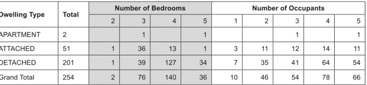
he Canadian telecom service operator provided data for 564 houses. he dataset contained energy and thermostat data (setpoints, actual temperatures, HVAC run-times) for 527 dwellings, motion/door (occupancy) data for 416 houses, and household characteristics data for 254 houses. Table 1 sum-marizes the household characteristics; the two dwellings were electrically heated and were removed from further analysis, all other dwellings were gas heated.
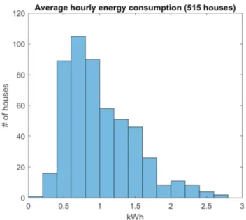
here were 515 houses that had energy consumption records for at least 8000 hours from March 2015 to February 2016 (inclusive). Figure 1 shows the distribution of average hour-ly energy use among those houses1; mean=1.05 kWh,
medi-an=0.90 kWh, standard deviation (SD)=0.56 kWh.
Furthermore, Table 2 shows the average hourly electricity consumption by number of household occupants. As expected, average total energy use increased systematically with the num-ber of occupants.
hese data are consistent with comparable studies, and add to our conidence that this sample is representative. Newsh-am et al. (2011) exNewsh-amined electricity data from 320 houses in Southern Ontario in 2008, and reported a mean hourly elec-tricity use of 1.0 kWh over a full calendar year. Other studies
1. Ten houses were excluded from this analysis because they were clear outliers (total energy use was three standard deviations above the mean).
Table 1. Characteristics of sample dwellings.
Dwelling Type Total Number of Bedrooms Number of Occupants
2 3 4 5 1 2 3 4 5
APARTMENT 2 1 1 1 1
ATTACHED 51 1 36 13 1 3 11 12 14 11
DETACHED 201 1 39 127 34 7 35 41 64 54
5. BUILDINGS AND CONSTRUCTION TECHNOLOGIES AND SYSTEMS
ECEEE SUMMER STUDY PROCEEDINGS 1005 5-065-17 NEW SHAM ET AL
conducted in Ontario report typical average hourly household electricity use of 1.0–1.2 kWh (Strapp et al., 2007; Navigant, 2008). Newsham et al. (2011) further reported that electricity use increased linearly with number of household occupants.
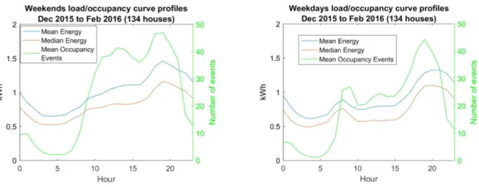
Figure 2 shows average hourly load and occupancy activity proiles for winter months, as an example, for weekdays and weekends separately. As expected, higher energy use was as-sociated with a higher frequency of occupancy-related events. On weekends the morning increase in electricity use was later and less pronounced than on weekdays. Average energy use de-clined during the middle of the day on weekdays because many homes are vacated during these hours, but this decline did not occur on weekends when daytime occupancy is more common; overall, energy use was higher on weekends than weekdays.
Disaggregation of Energy Use
REFRIGERATION AND PHANTOM LOAD USE
Some electrical loads, such as refrigerators and other plugged-in appliances (so called “phantom loads” or “base” or “standby” loads) draw energy continuously (at the hourly level). To esti-mate these loads in each house we examined electricity use dur-ing hours when HVAC was not operatdur-ing. We then rank-ordered these hourly loads and considered the 10th percentile value; this
served to exclude hours with the highest discretionary appliance use, while also eliminating hours with very unusually low con-sumption. his approach is likely to primarily identify consump-tion during typical overnight hours. Figure 3 shows estimates for all houses2; mean=0.35 kW, median=0.30 kW, SD=0.23 kW.
From 327 Southern Ontario houses from 2008, Birt et al. (2012) reported a result of 0.3 kWh/hour using a similar ap-proach. Nelson (2008) reported results of a similar study of~300 households in British Columbia, Canada, the average base load was 0.30 kW for single-family dwellings, and 0.15 kW for row houses. In 12 highly-instrumented households in Brit-ish Columbia, Nelson et al. (2014) reported an average baseload of 0.29 kW, the major contributors to which were refrigeration, computing and entertainment, and water heating (if applica-ble). By comparison, the estimates derived in our study appear credible. Typical average base loads for houses in Europe (based on measurements from >1000 households) are about half these values, consistent with lower electricity use compared to North America generally, with refrigeration comprising about half the total base load in Europe (Grinden & Feilberg, 2008).
AIR CONDITIONING (AC) USE
We considered summer data and hours in which there were no occupancy events (to reduce variation in the energy use due to discretionary appliance usage). he data were plotted (x-axis: fraction AC runtime/hr, y-(x-axis: kWh/hr total household energy use) and a robust regression analysis was performed3. 2. We also applied a further ilter, removing hours in which there were some oc-cupancy events, to provide extra assurance that there was minimal discretion-ary appliance use. This reduced the sample size substantially, but produced very similar results to Figure 3.
3. Given that run-time data were available directly from the thermostat, this was the most direct way to estimate AC size. Absent run-time data, AC size might be estimated by plotting electricity use vs. outside temperature, as described in Birt et al. (2012).
An example from one house is shown in Figure 4. here is con-siderable scatter in the data, relecting the variability across all electricity end-uses and all hours. Very low values of electricity use during high run-time hours might relect data communica-tion errors, or times when the thermostat called for cooling but when the AC unit was disconnected. Nevertheless, the regres-sion trend is obvious. Subtracting the regresregres-sion it at value “0” (AC was not running) from the it at value “1” (AC was running all hour) gives an estimate of the size of the central AC unit controlled by the thermostat, in kW.
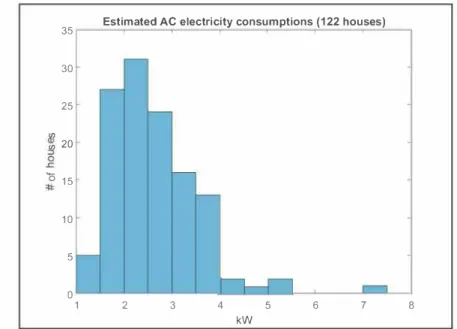
here were 122 houses with applicable data for which the R2
value of the regression was above 0.6, and for these the estimat-ed AC size (kWh per hour/hour=kW) is shown4 in Figure 5;
mean=2.63 kW, median=2.45 kW, SD=0.90 kW.
Direct measurement of 390 residential AC units in Ontario showed an average power draw of 1.93 kW (min. 0.99 kW; max. 5.01 kW) (KEMA, 2009), whereas Toronto Hydro (2016) guid-ance on energy use suggests 3.5 kW for a central air-condition-er. he mean value of 2.63 kW that we derived lies within this range, and by comparison, the estimates derived in our study appear credible. We can calculate the annual energy use for AC in each house by multiplying the estimated AC size by the total hours and partial hours of AC runtime5. Figure 6 shows the
esti-mated annual energy used for AC cooling for houses with suit-able data; mean=952 kWh, median=752 kWh, SD=792 kWh.
4. This includes the power draw of the central circulation fan.
5. We illed in missing data via the nearest-neighbour approach, based on: hour of day, and outside temperature.
Figure 1. Average hourly electricity consumption for sample dwellings.
Table 2. Average hourly electricity consumption by number of household occupants.
# of occupants 1 2 3 4 5
Figure 2. Average load and occupancy event proiles for the winter season (December 2015–February 2016) for the sub-set of houses with suitable data.
Figure 3. Estimate of refrigeration and phantom loads for all houses.
Figure 4. Example of regression used to make an AC size estimation for a single house, regression R2=0.79. 140 120 100 � 80 i 0 c
o
60 : 40 20Refrigeration and Phantom Loads (506 houses)
O ____JJJJJJJJ=��d
0 0.2 0.4 0.6 0.8
kW 1.2 1.4
1.6
5. BUILDINGS AND CONSTRUCTION TECHNOLOGIES AND SYSTEMS
ECEEE SUMMER STUDY PROCEEDINGS 1007 5-065-17 NEW SHAM ET AL
Newsham & Donnelly (2013) generated a statistical model for residential electricity and gas use based on a large sample of households across Canada. Using their coeicient for central cooling, and applying average cooling degree day values for To-ronto, yields an estimate of ~700 kWh/yr. Newsham & Donnel-ly (2013) quote other estimates of residential central AC energy use in Canada, including British Columbia at 346 kWh/yr and 1,963 kWh/yr for Quebec, both of which have a milder summer climate than Southern Ontario. By comparison, the estimates derived in our study appear credible.
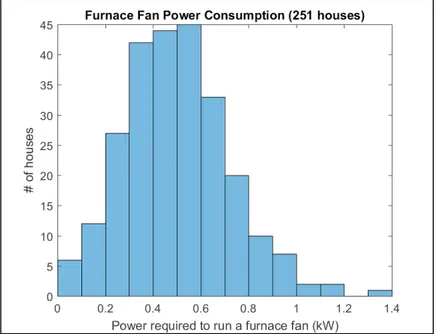
FURNACE FAN USE
Dwellings heated by natural gas in this pilot used a central furnace (typically in a basement), with warm air distributed throughout the dwelling using ducts and an electrically-pow-ered circulation fan. To disaggregate the furnace fan electricity
use, we employed a similar technique to the AC consumption estimation, considering records from the heating season during which no occupancy events were recorded. Figure 7 shows the estimated furnace fan power draw for all houses with suitable data6; mean=0.50 kW, median=0.49 kW, SD=0.22 kW.
he Canadian Centre for Housing Technology (CCHT) comprises full-scale single-family detached research houses built to standards similar to the current Ontario Energy Code. Measurements of the power draw of examples of both Perma-nent Split Capacitor (PSC) and Electronically Commutated Motor (ECM) type furnace fans at the CCHT showed their full
6. The furnace fan is a smaller load than AC, and thus more diicult to estimate. We tried limiting our estimates to houses where the regression R2 was >0.6. This reduced the sample size substantially, but produced very similar results to Figure 7.
35 Estimated AC electricity consumptions (122 houses) 30 25 ) 20 ) 0 15 10 5 0 1 2 3 4 5 6 7 8 kW
Figure 5. Estimate of AC size for the sub-set of houses with strong regression its.
output power was 0.49 kW and 0.28 kW, respectively (Gusdorf et al., 2002). he PSC type is the most common in residential applications. Consumer guidance on furnace fan wattage rang-es from 0.35–0.75 kW (Toronto Hydro, 2016; Consumer Re-ports, 2016). By comparison, the estimates derived in our study appear credible.
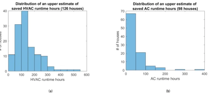
Potential Energy Savings from Additional Thermostat
Setback
More savings can result from additional thermostat setbacks during absence or night-time than those programmed in the houses, either because no setback7 was programmed at all, or
because the programmed setback was not as deep as it poten-tially could be. A smart thermostat, supported by occupancy information, could engage such setbacks automatically (e.g. Lieb et al., 2016). To estimate the upper limit of these sav-ings for the heating period, we summed all the HVAC runt-ime hours when the thermostat setpoint was above 18 °C, and
there were no occupancy-related events in the three previous hours8. For the cooling season, we summed the HVAC
runt-ime hours when the thermostat setpoint was below 25.5 °C
and there were no occupancy related events in the three pre-vious hours9.
Note, however, our analysis was limited to houses for which reliable occupancy event data were available. Reliability could have been compromised for several reasons, including: the oc-cupancy/door sensors were not installed; the sensors were
in-7. We use the generic term “setback” for both heating and cooling seasons. In the heating season, this means lowering the thermostat setpoint during absences or overnight, in the cooling season it means raising the setpoint.
8. Given that the occupancy-related sensors might not capture all occupant activ-ity, we chose three hours as an (arbitrary) safety factor to be conident that the house was indeed unoccupied.
9. 18 and 25.5 °C were guided by the setpoints reported in a survey of Canadian households (NRCan, 2010); they were within the range of reported values, but towards the more energy-eicient end of the range.
stalled but not in places where activity occurred; the sensor bat-teries failed; or, there was a wireless data transmission error.
Figure 8(a) shows the estimated additional HVAC runt-ime savings in the heating season, for houses with suitable data; mean=144.0 hours per house, median=127.5 hours, SD=92.1 hours. Figure 8(b) shows similar data for the cooling season; mean=48.4 hours, median=33.2 hours, SD=56.6 hours.
We consider this analysis an upper estimate of the potential savings in runtime hours for several reasons. First, the sugges-tion that setback could be deeper than 18/25.5 °C might not be
acceptable to the occupant. Second, we are suggesting that all run-time hours will be saved with these additional thermostat setbacks. In fact, if the absence is long enough that the internal temperature reaches the setback temperature the HVAC sys-tem will resume operation. Finally, when the resident returns there may be additional energy use in HVAC activity to recover to the occupied setpoint. he exact energy impact of these ef-fects depends on occupancy schedules, solar gains and other exterior conditions.
Some consideration needs to be given to how big the auto-mated setback should be, and to house temperature recovery time, given that the occupant may be returning to a tempera-ture they had not programmed. he safest choice is what might be termed a “shallow setback”, perhaps only 1 °C, which would
be unlikely to be noticed by a returning occupant, and is within the deadband and measurement error margin of many ther-mostats anyway.
Relative House Structure Thermal Characteristics
his analysis is based on a variant of the basic heat balance equation for a house, in the absence of solar gains (Eq. 1):
Figure 7. Estimated furnace fan power draw for all houses with suitable data.
∆�#=�� ��'− �# * + �#.* �* + �/ �*
5. BUILDINGS AND CONSTRUCTION TECHNOLOGIES AND SYSTEMS
ECEEE SUMMER STUDY PROCEEDINGS 1009 5-065-17 NEW SHAM ET AL
where,
∆Ti change in indoor air temperature in one hour
U integrated envelope heat loss characteristic due to con-ductive and iniltrative processes
A exposed area of building To outdoor air temperature Ti indoor air temperature
Qint internal heat gains (e.g. waste heat from appliances, oc-cupant metabolic heat)
Qf heat gains from furnace
Mt thermal mass characteristic (higher thermal mass means slower change in temperature for a given heat gain) his can be expressed as a simple linear equation (Eq. 2):
y = mx + c where, y = ∆Ti x = (To – Ti) m = UA/Mt c = (Qint + Qf)/Mt
From the thermostat data we know the indoor air temperature in any given hour and its change during that hour, and we know the outdoor air temperature from Environment Canada data, therefore, we can conduct a regression on these data and es-timate the m and c parameters. A relatively high value of m, meaning relatively high heat loss, indicates a relatively poorly insulated envelope, an envelope with relatively high air leakage, a relatively large envelope area10 or a house with relatively low
thermal mass, or a combination of all three.
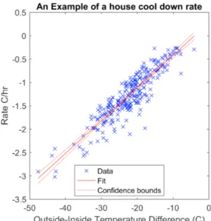
To estimate these parameters in the heating season, we looked at the time period when the house cooled down at night ater the night setback started. Note that in this situation Qf = 0 and c rep-resents internal gains (and thermal mass) only. For each house, the cool down time was recorded along with the average inside and outside temperature observed at that time (the cool down
10. Note, it might be possible to parse out the efect of envelope area with data on house size, supplied either by the homeowner or from a public database.
period was only recorded if the indoor temperature drop over-night was at least 1 °C). hus, for a single night, ∆T
i is the
tem-perature drop in the cool down period divided by the time that the cool down took, and (To–Ti) is the diference between the average outdoor and indoor temperatures during that period.
An example of a single night of time series data is shown in Figure 9. We identiied the beginning of the house cool down period at night-time when temperatures started falling con-sistently, 23:55 in the example in Figure 9. We identiied the end of the cool down period when the indoor temperature did not drop anymore and/or the furnace started, 03:37 in the ex-ample in Figure 9. he indoor-outdoor temperature diference was ((20.5+17.8)/2)–2.25=16.9 °C. he cool down rate was thus
2.7/3:42=0.73 °C per hour. Note that in the Figure 9 example the indoor temperature drop during cool down was very linear.
We did this for all nights with valid data for a single house. Finally, we performed a linear regression on this set of points to ind the amount of time it took for the house to cool down as a function of the temperature diferences between the inside and the outside. To limit the regression artefacts, we constrained the regression to output models with non-negative intercept11.
Figure 10 shows the resulting “rate vs. temperature diference” plot for all nights for the same single example house.
he best it regression line in Figure 10 was: Y=0.07*X+0.28; this generates the m (slope=0.07) and c (intercept=0.28) param-eters in Eq. 2. We then computed these paramparam-eters for all houses with suitable data, and the result is shown in Figure 11. Note that the houses with the largest slopes also tend to have the larg-est intercepts, sugglarg-esting common causes that afect both pa-rameters. For example, these could be houses with relatively low thermal mass, or relatively large houses that would tend to have larger envelope areas and higher internal gains. Nevertheless, for houses with low intercept values, there was a range of slopes, and those with larger slopes could be targets for energy eiciency programs designed to improve envelope performance.
11. A negative intercept would mean that the house keeps losing temperature even though the outside temperature is equal to the temperature inside the house, a physical impossibility.
Figure 8. Upper estimates of HVAC runtime hours savings due to additional setback in the (a) heating season, and (b) cooling season, for houses with suitable data.
(a) (b)
Conclusion
he growing availability of house performance data from smart thermostats, smart meters, and public databases ofers many possibilities for estimating various house characteristics and quantifying savings opportunities at the individual house level. Segmentation of household populations based on such estimates may be used to target energy eiciency programs to-wards houses most likely to beneit. In principle, this may in-crease program participation, and yield more beneit for a given program investment.
Data from a sample of typical houses in Ontario, Canada demonstrated some viable approaches for deriving such char-acteristics and opportunities related to end-use disaggrega-tion, automated thermostat setbacks, and thermal character-istics of the houses. he end-use disaggregation estimates were credible compared to other methods on similar house popula-tions: mean refrigeration and phantom loads were estimated as 0.35 kW, the mean central AC size was 2.63 kW, and the mean furnace fan power draw was 0.50 kW. For many houses, a hun-dred or more of hours of potential HVAC run-time could have
Figure 9. Indoor temperature cool down during night-time setback for a single house on a single night, showing derivation of parameters for our analysis.
Figure 10. Cool down rate vs. temperature diference for an example house over the heating season. The best it regression line is shown.
Figure 11. Estimated cool down rates of all houses with suitable data. The colours of each point represent the variability explained (R2) by
5. BUILDINGS AND CONSTRUCTION TECHNOLOGIES AND SYSTEMS
ECEEE SUMMER STUDY PROCEEDINGS 1011 5-065-17 NEW SHAM ET AL
natural gas use and overall energy use during the heat-ing season of CCHT research facility. Proceedheat-ings of Gas Technology Institute’s First Natural Gas Technologies Conference and Exhibition, (Orlando, FL).
Horizon Utilities Corporation. 2014. Energy mapping for de-livery of conservation and demand management (CDM) programs. Project Report, 13 pages.
KEMA. 2009. Ontario Power Authority 2009 peaksaver® residential air conditioner measurement and veriica-tion study. Report for OPA (Toronto Hydro). URL: http://www.powerauthority.on.ca/sites/default/iles/ new_iles/2009/2009%20peaksaver%20Residential%20 Air%20Conditioner%20Measurement%20and%20Verii-cation%20Study.pdf.
Kwac, J.; Flora, J.; Rajagopal, R. 2014. Household energy con-sumption segmentation using hourly data. IEEE Transac-tions on Smart Grid, 5 (1), 420–430.
Lieb, N.; Dimetrosky, S.; Rubado, D. 2016. hriller in Asi-lomar: battle of the smart thermostats. Proceedings of ACEEE Summer Study on Energy Eiciency in Buildings (Paciic Grove, CA), 2.1–2.13.
Navigant. 2008. Evaluation of Time-of-Use Pricing Pi-lot. Presented to Newmarket Hydro, and delivered to the Ontario Energy Board. URL: http://www.oeb.gov. on.ca/OEB/Industry+Relations/OEB+Key+Initiatives/ Regulated+Price+Plan/Regulated+Price+Plan+-+Ontario+Smart+Price+Pilot.
Nelson, D.J. 2008. Residential baseload energy use: concept and potential for AMI [Advanced Metering Infrastruc-ture] customers. Proceedings of ACEEE Summer Study on Energy Eiciency in Buildings (Paciic Grove, CA), 2.233–2.245.
Nelson, D.J.; Berrisford, A.J.; Xu, J. 2014. MELs: What have we found through end-use metering? Proceedings of ACEEE Summer Study on Energy Eiciency in Buildings (Paciic Grove, CA), 9.274–9.285.
Newsham, G.R.; Birt, B.J.; Rowlands, I.H. 2011. he Efect of Household Characteristics on Total and Peak Electricity Use in Summer. Energy Studies Review, 18, (1), 20–33. Newsham, G.R.; Donnelly, C.L. 2013. A Model of Residential
Energy End-Use in Canada: Using Conditional Demand Analysis to Suggest Policy Options for Community En-ergy Planners. EnEn-ergy Policy, 59, 133–142.
NRCan. 2010. 2007 Survey of Household Energy Use (SHEU-2007) Detailed Statistical Report. URL: http://oee.nrcan. gc.ca/publications/statistics/sheu07/pdf/sheu07.pdf. NRCan. 2016. Energy Use Data Handbook. Natural Resources
Canada. URL: http://oee.nrcan.gc.ca/corporate/statis-tics/neud/dpa/data_e/downloads/handbook/pdf/2013/ HB2013e.pdf.
Parekh, A.; Mullally-Pauly, B.; Riley, M. 2000. he EnerGuide for houses program: a successful Canadian home energy rating system. Proceedings of ACEEE Summer Study on Energy Eiciency in Buildings (Paciic Grove, CA), 2.229–2.240.
Rotondo, J.; Johnson, R.; Gonzalez, N.; Waranowski, A.; Badg-er, C.; Lange, N.; Goldman, E.; FostBadg-er, R. 2016. Overview of existing and future residential use cases for connected thermostats. Report for the Building Technologies Oice, US Department of Energy. URL: https://energy.gov/sites/ been saved by automatically adjusting the thermostat when no
occupancy was detected for an extended period. Further, ana-lysing the rate at which a house cools down overnight provides an indicator of relative thermal eiciency. Doubtless, other en-ergy eiciency insights may be gained by further analysis of similar data by researchers with a knowledge of building phys-ics, occupant behaviour, and data science. For example, house-holds whose electricity demand has greater coincidence with the system-wide peak could be identiied, and be targeted for demand-response programs.
he next step should be to validate remotely-derived house-hold characteristics by comparison to on-site physical audits. If successful, future market research should test the hypothesis that targeting programs based on these estimates and segmen-tation does indeed lead to program beneits.
References
Accenture. 2013. Realizing the Full Potential of Smart Metering. URL: https://www.accenture.com/
t20160413T230144__w__/us-en/_acnmedia/Accenture/ Conversion-Assets/DotCom/Documents/Global/PDF/In- dustries_9/Accenture-Smart-Metering-Report-Digitally-Enabled-Grid.pdf.
Albert, A.; Rajagopal, R. 2015. hermal proiling of residential energy use. IEEE Transactions on Power Systems, 30 (2), 602–611.
Armel, K.C.; Gupta, A.; Shrimali, G.; Albert, A. 2013. Is dis-aggregation the holy grail of energy eiciency? he case of electricity. Energy Policy, 52, 213–234.
Birt, B.J.; Newsham, G.R.; Beausoleil-Morrison, I.; Armstrong, M.M.; Saldanha, N.; Rowlands, I.H. 2012. Disaggregating categories of electrical energy end-use from whole-house hourly data. Energy and Buildings, 50, 93–102.
Considine, T.J.; Sapci, O. 2016. he efectiveness of home energy audits: a case study of Jackson, Wyoming. Resource and Energy Economics, 44, 52–70.
Consumer Reports. 2016. Power play. URL: http://www.con-sumerreports.org/cro/resources/images/video/wattage_ calculator/wattage_calclulator.html.
Du Bois, D. 2014. How eiciency is learning about market segmentation from internet giants and political cam-paigns. Greentechmedia, October 30th. URL: https://www.
greentechmedia.com/articles/read/how-energy-eicien- cy-marketers-are-learning-about-market-segmentation-from.
Ehrhardt-Martinez, K. 2012. A comparison of feedback-in-duced behaviors from monthly energy reports, online feedback, and in-home displays. Proceedings of ACEEE Summer Study on Energy Eiciency in Buildings (Paciic Grove, CA), 7.60–7.74.
Frondel, M.; Vance, C. 2013. Heterogeneity in the efect of home energy audits: theory and evidence. Environmental and Resource Economics, 55, 407–418.
Grinden, B.; Feilberg, N. 2008 Analysis of monitoring cam-paign in Europe. Report D10 of REMODECE project. URL: http://remodece.isr.uc.pt/downloads/REMODECE_ D10_Nov2008_Final.pdf.
Gusdorf, J.; Swinton, M.C.; Entchev, E.; Simpson, C.; Cas-tellan, B. 2002. he impact of ECM furnace motors on
servation and eiciency programs. Applied Energy, 115, 25–36.
Toronto Hydro. 2016. Appliance Usage Chart. URL: http:// www.torontohydro.com/sites/electricsystem/residential/ yourbilloverview/Pages/ApplianceChart.aspx.
Zeifman, M.; Roth, K. 2016. Residential remote energy perfor-mance assessment: estimation of building thermal param-eters using interval energy consumption data. Proceedings of ACEEE Summer Study on Energy Eiciency in Build-ings (Paciic Grove, CA), 12.1–12.12.
Acknowledgements
his project was funded by the Canadian telecom service opera-tor referred to in the text, and by the National Research Council Canada under its High Performance Buildings Program. he authors are grateful for the help provided by Ryan Shaw and Eshna Kaul, and by Elias Puurunen (Northern HCI Solutions Inc.).
prod/iles/2016/12/f34/Overview%20of%20Existing%20 Future%20Residential%20Use%20Cases%20for%20 CT_2016-12-16.pdf.
Schmidt, L. 2012. Online smart meter analysis achieves sus-tained energy reductions: results from ive communities. Proceedings of ACEEE Summer Study on Energy Eicien-cy in Buildings (Paciic Grove, CA), 12.264–12.276. St. John, J. 2013. Putting energy disaggregation tech to the test.
November 18th. URL:
https://www.greentechmedia.com/ar-ticles/read/putting-energy-disaggregation-tech-to-the-test. Strapp, J.; King, C.; Talbott, S. 2007. Ontario Energy Board
Smart Price Pilot Final Report. Prepared by IBM Global Business Services and eMeter Strategic Consulting for the Ontario Energy Board. URL: http://www.oeb.gov. on.ca/OEB/Industry+Relations/OEB+Key+Initiatives/ Regulated+Price+Plan/Regulated+Price+Plan+-+Ontario+Smart+Price+Pilot.
Taylor, N.W.; Jones, P.H.; Kipp, M.J. 2014. Targeting utility customers to improve energy savings from