An analytic structure for sustainable energy in competitive electricity markets

An Analytic Structure for Sustainable Energy in Competitive Electricity Markets by

Arnob K. Bhattacharyya

Submitted to the Department of Electrical Engineering and Computer Science

in Partial Fulfillment of the Requirements for the Degrees of

Bachelor of Science in Electrical Engineering and Computer Science

and Master of Engineering in Electrical Engineering and Computer Science

at the

MASSACHUSETTS INSTITUTE OF TECHNOLOGY May 9, 2003

V Massachusetts Institute of Technology 2003. All rights reserved.

OF TECHNOLOGY 0- .

JUL 3 0 2003

LIBRARIES

Author

Department of Electrical Engineering and omputer Science D n ay 9, 2003

Certified by

Stephen R. Connors Coordinator -Multidisciplinary Research Director, Analysis-Group for Regional Electricity Alternatives Thesis-j.ppervisor

Accepted by

An Analytic Structure for Sustainable Energy in Competitive Electricity

Markets

by

Amob Bhattacharyya

Submitted to the Department of Electrical Engineering and Computer Science on May 9th 2003 in

partial fulfillment of the requirements for the degrees of Bachelor of Science in Electrical Engineering and Computer Science and Master of Engineering in Electrical Engineering and Computer Science

ABSTRACT

Vast resource requirements and copious production of emissions and their associated social and environmental concerns have made the electric utility sector a hot topic of several debates. Some of the core issues include increased competition, increased population growth accompanied by increases in demand, and global climate change. Although this is a global problem, we address the issues presented on a more regional level by looking at the Scandinavian utility sector. In this thesis, PROSYM, a chronological electric power production costing simulation computer software package, is tested as a possible model to be used for a sustainability project. It is determined that PROSYM's hydro logic is inept and suggestions are made as to how to improve the model to handle a system with a large amount of hydro generation. With these fixes in place, we then shift focus to the benefits and costs of adding alternative energy sources to the system. Multiple simulations are run to test the feasibility of adding wind to the Scandinavian system. Emissions and transmission line capacities are analyzed to measure the effect of this added generation. Having looked at both a model and an alternative energy source, detailed suggestions are made as to the requirements for a sustainable production model. Model, data, and scenario requirements are discussed thoroughly in an effort to attract multiple stakeholders and to engage them in a debate over the critical issues and the future direction for a planning project in Scandinavia.

Thesis Supervisor: Stephen R. Connors

Title: Coordinator - Multidisciplinary Research

Acknowlegdements

I would like to thank my advisor and mentor Stephen R. Connors for his unrelenting support. He provided the guidance and inspiration I needed to complete the work, by constantly taking time out of his busy schedule to design work arounds for problems encountered. Furthermore, the input from Audun Botterud and Kaare Gether helped to develop the thesis making it more

comprehensive. Audun worked on several projects for more than the span on a year, yet he always found time to brainstorm with me. Thanks!!

I would also like to thank Prasad Ramanan for several late night discussions that made me look at problems in a different light. His guidance helped me to sail through my graduate studies. It has

truly been a privilege to work with him throughout my MIT career. I wish you the best in your career and your life.

Lastly, to my family who has been always supportive and understanding, I couldn't have done it without you. I owe all my success to your love.

Table Of Contents

INTRODUCTION 9

2 OVERVIEW OF MODELLING AND DATA ISSUES 11

2.1 The PROSYM and EMPS Models 11

2.1.1 PROSYM 11 2.1.2 EMPS 11 2.1.3 PROSYM vs. EMPS 12 2.1.4 Current Work 13 2.2 Geographic Division 13 2.3 Load Division 14 2.3.1 Norway 14 2.3.2 Sweden 15 2.3.3 Denmark 16 2.4 Transmission Lines 17 2.5 1 Hydro Production 18

2.6 Heat Rates for Thermal Plants 19

2.7 Modeling Germany, Finland, Poland, and Russia 21

2.8 Profiles for Nuclear and CIP Plants 22

3 1IYDRO SCIIEDULING AND TIlE PROSYM MODEL 25

3.1 Hydro Scheduling Methodology 25

3.1.1 Hydro Scheduling Issues 25

3.1.2 External Hydro Scheduling 25

3.1.3 Scenario Selection and Data Preparation 26

3.21 lydro Scheduling Results 27

3.2.1 Varying Hydro/Flat Thermal Results 27

3.2.2 Flat Ilydro/Varying Thermal Results 29

3.2.3 Varying I lydro/Thermal Results 30

3.3 Improving the Hydro Scheduling Methodology 33

3.3.1 Representative Weeks 33

3.3.2 Results of Ilydro Scheduling Methodology for Representative Weeks 35

3.3.3 Factor Adjustment for Run-of-River Content 38

3.3.4 Results of Factor Adjustment for Run-of-River Content 40

3.4 Pitfalls and Alternatives 42

3.4.1 Pitfalls of Hydro Scheduling Methodology 42

3.4.2 Alternatives 43

4 INTEGRATING WIND INTO TIE ANALYSIS OF TIE SCANDINAVIAN SYSTEM 45

4.1 Wind in Norway 45

4.1.1 Load Characteristics in Norway 45

4.1.2 Wind Characteristics in Norway 48

4.2 Converting Wind to Power 49

4.2.1 Converting Data to I lub Height 49

4.2.2 Analyzing Wind in Norway 50

4.2.2.1 NorwayS 50

4.2.2.2 NorwayW 51

4.2.3 Estimating the Power Curve 4.2.4 Total Power

4.2.5 Power Surface Curves 4.2.6 Load Surface Curves 4.3 PROSYM Simulations

4.3.1 Transmission Lines 4.3.2 Transmission Area Prices 4.3.3 CHP Generation

4.3.4 Hydro Scheduling 4.4 Transmission Line Solution 4.5 Issues with Wind

4.6 Conclusions

5 MODEL AND DATA REQUIREMENTS FOR A PLANNING PROJECT IN

ENERGY

5.1 The Optimal Model

5.1.1 System Boundary & Time Resolution 5.1.2 Economics 5.1.3 Wind 5.1.4 H ydro 5.1.5 Thermal 5.1.6 Hydro/Thermal Coordination 5.1.7 Price-Flexible Load 5.1.8 Cost/Bid-based Dispatch 5.2 Data 5.2.1 Load Data 5.2.2 Hydro Data 5.2.3 Wind Data 5.2.4 Heat Data 5.2.5 Plant Data 5.2.6 Database Organization 5.2.7 Database Security 5.3 Scenario Selection

5.3.1 Supply Side Technology Options 5.3.2 Demand Side Technology Options 5.3.3 Bidding Strategies

5.3.4 Emission Trading

5.4 Multi-Attribute Trade-Off Analysis 5.5 Conclusions CONCLUSION REFERENCES 54 57 58 60 60 61 63 65 65 66 66 67 SUSTAINABLE 69 69 69 70 70 70 71 72 72 74 74 74 74 75 75 75 76 78 78 78 79 79 80 81 82 83 85

INTRODUCTION

Environmental emissions, increasing demand for power, and vulnerability of electric power networks have increased concerns about the sustainability of the electric sector. These issues not only play an important role in the choice of future options for system development, but in current operation as well. It is important that we understand that the issues mentioned above are not disjointed. A solution that decreases environmental emissions at the risk of higher vulnerability of the power network is not robust. Any proposed solution will be complex, will have to be implemented with finite resources, and will have some degree of impact on society as a whole.

Decision makers and planners in the electricity sector are searching for an elegant solution to the sustainability problem by addressing the issues mentioned above. There are an ample number of suggestions for solving this problem. Technological advances in power generation, power storage, end-use efficiency, and load management have provided us with both demand side and supply side solutions. The key is to accurately model these new technologies and to use them effectively to benefit the system in the present and the future. With the emergence of policy measures to control emissions and increased competition, these new technologies must be flexible. They must adapt to constraints that change rapidly and unpredictably.

Thus, any solution to this problem must balance the social, economic, and environmental dimensions of sustainable development. They must contribute to the management of risk and the improvement of flexibility, in order to avoid serious disruption of the energy system [I]. However, social concerns and regulatory policies which express themselves to govern system operation can change quickly. Changes in technology and public concern are reflected by changes in the regulatory and decision-making process, and policy options have proliferated, including emissions trading and taxes and various structures for increased competition. It is left up to the decision makers to deal with the conflicts of interest which exist between technological appropriateness, social acceptance, economic soundness and responsibility towards future generations, with the goal of social and economic development which achieves or maintains a high standard of living and improves quality of life [2].

As the above discussion has outlined, there is a need for research that will address the problems related to sustainability and the electric utility sector on the technical, systems, and decision-making levels.

There are several goals for this project. The idea is to involve a wide range of participants from the electricity sector, utility sector, environmentalists, and customers and to engage them in a debate of the current issues. It is important to identify and implement a wider range of measures that will serve as accurate indicators of sustainability. Improved modeling tools that simulate electric system operation under competition, and include transmission and distribution effects are essential to a project in sustainability. Analyzing technology options that are considered 'next generation' is of importance as this will give us insight into the limits of the current system.

These are some of the end goals for this project. We need to enumerate some of the more immediate goals that will help us reach these end goals. The most important of these goals is the gathering of data that describes the Scandinavian electricity market accurately and effectively. The next is to gather a group of stakeholders who can enlighten us as to the most critical issues and those that can be addressed at a later time. Using this information a set of scenarios must be developed that analyzes a wide array of both supply and demand side options. Finally, a model must be chosen to test these scenarios and to further identify and refine the goals for this planning project.

We have attempted to address some of the goals mentioned above in this paper. The first major issue that we tackled was the selection and examination of a possible model for the project. Using a minimal data set, we tested the model to determine its feasibility for the project. After analyzing the model, we present possible improvements to enhance the functionality of the model in Chapter 2. While testing the model, meetings were held with possible stakeholders to determine particular areas of interest. One area of interest was chosen and researched quite thoroughly and is presented in Chapter 3. Chapter 4 integrates both the previous chapters and presents the requirements for a model that is to be used in this planning project. The chapter also discusses possible scenarios that should be explored and tested once a model has been chosen. Finally, we conclude and reiterate our findings.

2 OVERVIEW OF MODELLING AND DATA ISSUES

2.1 The PROSYM and EMPS Models 2.1.1 PROSYM

The electric power system in Scandinavia was simulated using the PROSYM model. PROSYM is a chronological model that represents the operation of several individual generating units which serve customer electricity demand on an hourly basis. As a general matter, the units with lower operating costs have priority in the dispatch over higher cost units, so that the total cost of operating the system is minimized. The model also recognizes generator operating constraints such as minimum down time and maximum ramp rates as well as transmission constraints between each of the individual "transmission areas" in the study region. In PROSYM, the electric industry is divided into a number of interlinked transmission areas, which correspond to the utilities' transmission capabilities and geographic boundaries; there are eight transmission areas in the three country region used in this analysis [3].

2.1.2 EMPS

EMPS has been developed for optimization and simulation of hydro-thermal power systems with a considerable share of hydropower. It takes into account transmission constraints and hydrological differences between major areas or regional subsystems. The EMPS model optimizes the utilization of storage capacity (hydropower, gas, emission quotas) in relation to demand and alternative sources of supply. The model has been developed for studying the operation of the Nordic and European power systems, and may also include gas markets and emissions quotas. The model is well suited for simulating the utilization of national or international energy resources, the interaction between hydropower and thermal-based generation, and e.g. the interaction between a gas- and an electricity market. Several hundred production units may be represented in a number of subsystems which may e.g. represent parallel markets for electricity and gas. Among available results are simulated market prices, generation, consumption and trade as well as emissions and economic results. At present, the model is frequently used for forecasting spot price development [4].

2.1.3 PROSYM vs. EMPS

Time resolution: PROSYM has an hourly while the EMPS model has a weekly time resolution. It

is therefore possible to add more detailed operational constraints with the Prosym model.

Thermal description: PROSYM allows the modeling of thermal plants in a very detailed fashion,

using max/min capacity, heat rates, ramp rates, start up/shut down costs, and variable operating costs. The EMPS model represents the thermal generation simply with marginal costs and available capacity.

Hydro description: The EMPS model has a detailed description of the optimization of hydropower

generation including all hydropower plants in the system. The network of waterways is also represented in the model. The Prosym model has no long-term optimization of hydropower, but dispatches the available hydro energy throughout the week, using internal hydro logic. Each single hydro unit can in theory be represented, but waterways and run of water between plants are not represented in the model. By using the EMPS model for long-term and Prosym for short-term dispatch of resources we should, at least in theory, end up with a good hydro description.

Transmission: The EMPS model divides Scandinavia into 15-20 areas and normally applies simple

constraints on the weekly energy transport between the areas. It is possible to add an additional DC loadflow module to represent the physical flow with more detail. PROSYM can handle up to 10 areas with hourly constraints on the transport capacity between areas.

Market design: Prosym can simulate a bid-based market, with possible strategic behavior from

participants with market power. The EMPS model does not have this option and aims at minimizing total cost by optimal use of the hydro reservoirs. In Prosym we can also represent ancillary services like reserve requirements. This may not be important in a system with more than

50 % hydropower.

Outages: In Prosym outages can be drawn from a probability distribution. In the EMPS model the

2.1.4 Current Work

The most crucial element of our work is to compile all necessary data, which include demand data, heat rates for thermal plants, weekly energy values, and fuel ratios for CHP plants that use two or more fuels. The next step is to determine scenarios to test in the short- and long-term. This is important as there are several issues that need to be considered and they must be compiled in an intelligible manner that will allow easy analysis of the results. Next, simulations spanning 1-year to 30-years into the future must be run and results must be collected and analyzed. Running these simulations allow us to learn the intricacies of the model, as well as its constraints. Then a different set of scenarios must be run and the results of these scenarios must be compared with previously collected results. This process is repeated until all alternatives have been exhausted.

2.2 Geographic Division

To proceed in our study of the Scandinavian area using the PROSYM model, the first step was to reduce the aggregate nature of the data. To accomplish this, we began by dividing each country in our model into distinct transmission areas. Thus, Norway was divided into four sub-areas, Sweden into two sub-areas and Denmark into two sub-areas. In the EMPS model, Norway consisted of twelve distinct areas. We tried to choose sub-areas so that the main bottlenecks in the system are still represented. This led us to reduce the twelve sub-areas into four as shown below.

Glomma Ostland Sorost

Hallingdal Norway South

Telemark Sorland

Vestsyd Norway West

Vestmidt

Norgemidt Norway Mid

Helgeland

Troms Norway North

Finnmark

Sweden and Denmark were divided into two sub-areas, Sweden North and South and Denmark East and West. These divisions were the same as those in the EMPS model for Sweden and Denmark. Once these divisions had been determined, the next step was to divide the aggregate load amongst the newly created areas.

2.3 Load Division 2.3.1 Norway

From the EMPS model, we acquired data for each of the twelve areas in Norway for 1999. We aggregated the data for the twelve sub-areas into the PROSYM areas that were created. The data from the EMPS model was quite detailed, as it divided the demand for each of the twelve areas in Norway into three parts, an industrial, residential, and price-flexible part, but has an hourly time resolution. As we aggregated the data into the four PROSYM areas, we were able to maintain the same level of detail as the EMPS model. This allowed us to extract ratios for the industrial, residential, and price-flexible parts of the load for each of the four PROSYM areas. The sum of these three parts for each area was the fraction of the total load that was assigned to that area. We combined the residential and price-flexible ratios into one; however the industrial was not easily combinable. Given that most of the industry in Norway is heavy industry which is running all the time and requires an almost constant amount of electricity, the total industrial load was subtracted from the aggregated Norwegian load. The Norwegian load, minus the industry, was then divided into the four PROSYM areas using the combined residential and price-flexible ratios. Once this was complete, the fraction of the total industrial load for each area was added back to create four separate demand profiles for the four PROSYM areas.

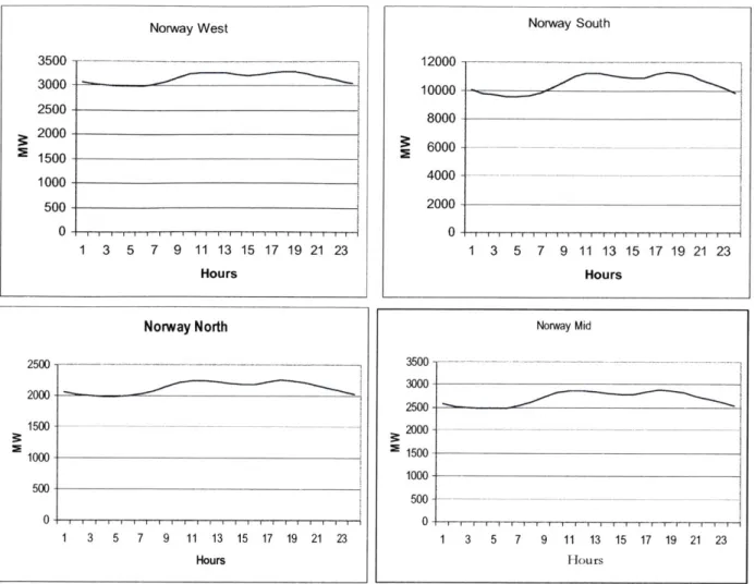
The figures below shows the total Norwegian load broken up into four separate areas for Jan. 2 0th,

Norway West 3500 -- - - - - --- - ---- - - - - -,_ 3000 - 2500-2000 1500- 1000- 500-1 3 5 7 9 11 13 15 17 19 21 23 Hours Norway North 2500 -- - - - -- - -2000 1500 -- _ - - 1000-500 1 3 5 7 9 11 13 15 17 19 21 23 Hours Norway South 12000 - _- -- _-- -_- -- 10000-8000 6000 - - --- - - -4000 --2000 1 3 5 7 9 11 13 15 17 19 21 23 Hours Norway Mid 3500 --- -A 3000 2500 - 2000---m 1500 1000 500 ---0 1 3 5 7 9 11 13 15 17 19 21 23 Hours

Figure 2-1: Variation in demand over a period of 24 hours in Norway.

As can be seen from above, the demand follows the same pattern in all four areas. This is because they are all based on the same aggregate hourly load data for Norway for 2001. Demand in all areas has a bi-modal profile. The first peak occurs at approximately noon, after which demand decreases slightly. We see that demand then rises to a second higher peak at approximately 5 in the evening, when people get home and start preparing dinner. From the graphs above, we see the Norway South has the largest load compared to the other areas as it is compromised of six sub-areas with a denser population.

2.3.2 Sweden

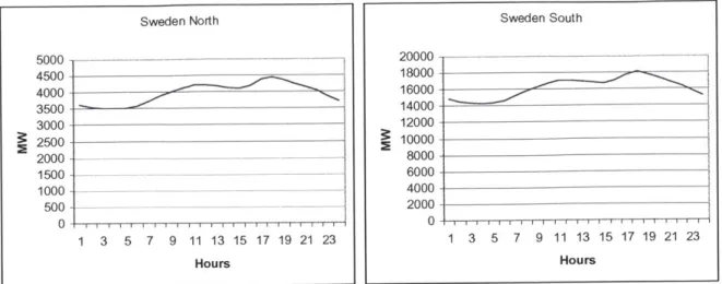
For Sweden, we also acquired data from the EMPS model. Since Sweden is modeled as North and South in the EMPS model, we directly determined the fraction of the total load for each area. With these ratios, we divided the 2001 data into North and South. Below is the graph of demand in the

Sweden North 5000 -4500 4000- 3500- 3000- 2500- 2000---1500 - - ---100 0 - -- - - - -500 -_--- __ 0 1 3 5 7 9 11 13 15 17 19 21 23 Hours Sweden South 20000 -- --- - _---18000 16000-. 14000 12000 10000 8000 6000 4000 2000 0 1 3 5 7 9 11 13 15 17 19 21 23 Hours

Figure 2-2: Variation in demand over a period of 24 hours in Sweden.

As can be seen from the graphs above, both Sweden North and Sweden South follow the same pattern. Similar to Norway, Sweden's demand profile is bimodal. Demand reaches its first maximum at approximately noon, decreases a bit for the following 3 hours and then reaches a new higher maximum at approximately 5 in the evening. It is obvious that Sweden South has a much higher load than Sweden North.

One point to take note of for both Norway and Sweden is that these demand profiles were artificially created from real data. That is, we have applied our own ratios to separate the load into separate parts to create different demand profiles. These ratios were extracted from EMPS input data, but may not be entirely accurate.

2.3.3 Denmark

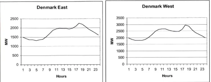
For Denmark, we acquired real historical data for East and West from Nord Pool. This means that we did not apply any ratios to the total demand to break them into their respective parts. The data in the figure below is therefore real data, and that explains why they have slightly different shapes, as opposed to the sub-areas in Norway and Sweden. Below is the graph of demand in the two areas of Denmark for January 2 0th,2001.

Denmark East 2500- - - - --- 2000-1500 1000 - - - -- _ 500-0 , 1 3 5 7 9 11 13 15 17 19 21 23 Hours Denmark West 3500---3000 2500- -2000 S1500-1000 500 0 1 3 5 7 9 11 13 15 17 19 21 23 Hours

Figure 2-3: Variation in demand over a period of 24 hours is Denmark.

Once again we see that the demand in Denmark East and West follow the same pattern. Similar to Norway and Sweden, Denmark's demand profile is bimodal. The first peak occurs at noon and the second higher peak occurs at approximately 6 in the evening. We also notice that the demand profile in Denmark is not as smooth as the other two countries. This can be attributed to the fact that this is real data. Also, Denmark is different from the other two countries as its load is almost evenly shared between East and West.

2.4 Transmission Lines

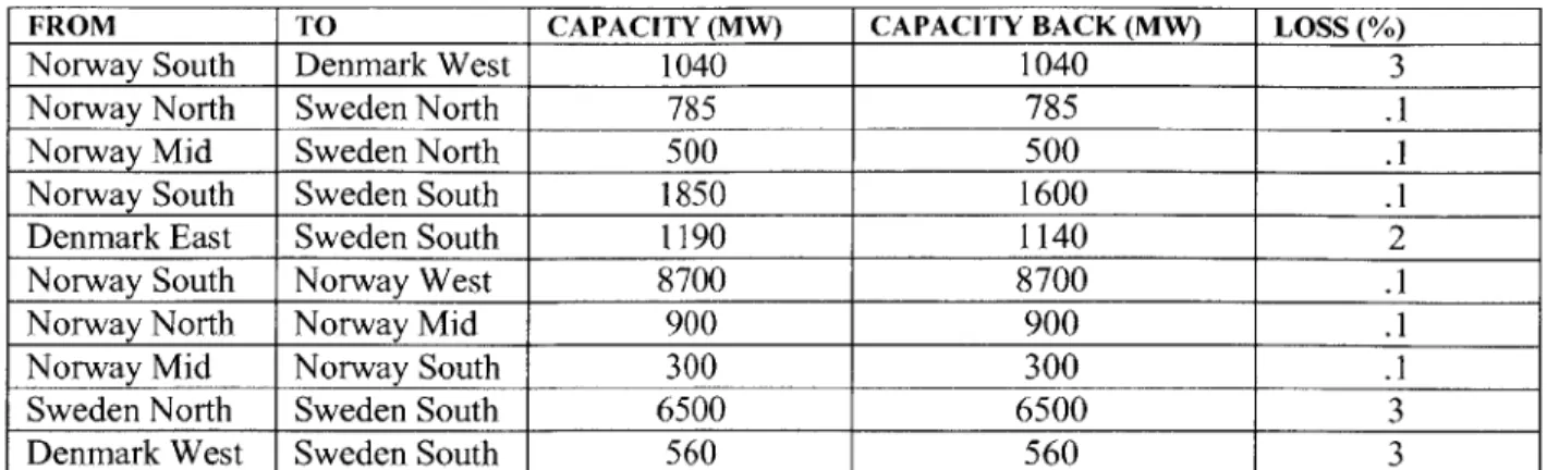
The transmission lines were modeled with the help of the EMPS model. The model had a list of all lines between the various areas, their MW capacity, loss rate, and duplex characteristics. Since we reduced the number of Norwegian areas from twelve in the EMPS model to four in the PROSYM model, some transmission lines needed to be aggregated. For example, Norway South has one transmission line that is an aggregate of all the transmission lines to the six individual sub-areas that it is composed of. This single transmission line is equivalent in capacity, loss rate, and duplex characteristics to all the transmission lines entering and leaving the six sub-areas comprising Norway South. Transmission lines were created in a similar fashion for the rest of Norway. Since Sweden and Denmark were represented the same way as the EMPS model, no aggregation was needed for lines leaving those two countries. Below is a table of the all the links in the PROSYM model.

FROM TO CAPACITY (MW) CAPACITY BACK (MW) LOSS (%)

Norway South Denmark West 1040 1040 3

Norway North Sweden North 785 785 .1

Norway Mid Sweden North 500 500 .1

Norway South Sweden South 1850 1600 .1

Denmark East Sweden South 1190 1140 2

Norway South Norway West 8700 8700 .1

Norway North Norway Mid 900 900 .1

Norway Mid Norway South 300 300 .1

Sweden North Sweden South 6500 6500 3

Denmark West Sweden South 560 560 3

Table 2-2: Transmission lines with associated loss rates between the transmission areas

2.5 Hydro Production

For hydropower we had access to weekly inflow statistics at Sintef Energy Research (SEfAS) for

both Sweden and Norway. The hydrological inflow series usually run from 1930 until 1990, so we

had sufficient statistical material for hydropower. In the EMPS model these series are used for

long-term stochastic optimisation of the storable hydropower generation. The time resolution in

the EMPS model is one week, and the optimisation usually takes place over a time period of I to 5 years. We used the EMPS model for long-term hydropower scheduling purposes in our trade-off

analysis, but we intended to use PROSYM for more detailed modelling with hourly time

resolution. We therefore needed to prepare the weekly results for hydropower generation from the

EMPS model so that they could be transferred to the PROSYM model. PROSYM requires a

weekly or monthly available hydropower production as input, and allocates the energy between the hours of the week, using specific logic for hydropower. The level of detail and complexity applied in this logic is flexible. The simplest and fastest way is to let the available hydropower be

scheduled in order to meet the demand as much as possible during high demand hours in the

system, and therefore level out the demand met by thermal units. The model can also optimize the hydropower generation through iterations based on an assessment of the marginal value of water in

the reservoirs. In the last case water values from the EMPS model can possibly be used as initial marginal values of the water in PROSYM.

The PROSYM model treats the weekly/monthly hydro generation as a deterministic variable. We will therefore need to create a set of scenarios to incorporate the uncertainty in hydro inflow into

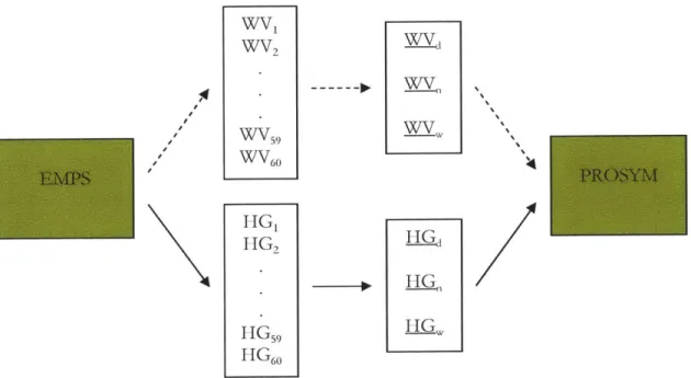
our model. Figure 2-4 illustrates how this can be done, by reducing the simulated values of weekly hydro generation and possibly also water values from EMPS, into for instance three scenarios for the availability of hydro energy in the power system. The methodology described here is directly applicable for the storable part of the hydropower generation. The non-storable part of the inflow can also be modelled in the same way, but with no flexibility in how to dispatch the energy over the week. We therefore represent the run of river fraction of the hydropower as minimum weekly capacities in PROSYM. Alternatively, run-of-river generation can also simply be modelled as a reduction in the demand.

, WV1 WV? WV59 WV60 HGI HG₂ HG₅₉ HG₆₀ W~d WVI WV HG, HG, 4

Figure 2-4: The transfer of weekly hydropower data from the EMPS model to the PROSYM model: a) Extraction of simulated weekly results for hydro generation (HGj) and possibly also water values (WVi) from the EMPS model. b) Reduction to three (or more) hydro scenarios (dry-d, normal-n, wet-w). c) Input of hydro scenarios to the PROSYM model.

Unfortunately, we have not been able to obtain plausible results with the built-in hydropower logic in PROSYM. Therefore, we have developed a logic that will treat the hydro power outside of the PROSYM model, as further described in Chapter 2.

2.6 Heat Rates for Thermal Plants

few levels of production and the associated incremental heat rate to run at those production levels.

The second is an average method for which we specify a level of production and an associated average heat rate for that level. And lastly, a coefficient option which allows us to specify

coefficients to create a heat rate curve. As we did not have detailed information available, we

decided to use a flat average heat rate curve. This means that the efficiency of the plant remained

constant at all levels of production. As production is increased, the cost associated with production

is directly related to the cost of fuel. The heat rate determines the initial marginal cost, but has no

bearing on the cost as production is increased from the minimum to the maximum level. As more

data becomes available we may switch to other options of modeling heat rates.

Sweden's nuclear and coal plants were assigned values to create a flat average heat rate curve.

Since there was no readily available data on heat rates for nuclear and coal plants, an average heat

rate for similar nuclear and coal plants was assigned to Sweden's plants. For Sweden's CHP

plants, average heat rates between 8000 GJ/GWh and 10000 GJ/GWh were assigned. As more

data becomes available these numbers will become more precise. For Denmark, data was

extracted from the EMPS model for all CHP plants leading to average heat rates ranging from

8,000 GJ/GWh to 65,000 GJ/GWh.

Below is a table of the various thermal plants in Sweden and Denmark.

Sweden Denmark

Plant Type Capacity (MW) Location Plant Type Capacity (MW) Location

Nuclear 9500 South CHP 400 West

CHP 635 South CHP 616 West

CHP 642 South CHP 700 West

CHP 641 South CHP 681 West

CHP 300 South CHP 700 West

CHP 170 South CHP 633 West

Com. Turbine 180 South CHP 1374 West

Com. Turbine 415 South CHP 250 East

CHP 151 North CHP 522 East CHP 1382 East CHP 500 East CHP 249 East CHP 166 East CHP 700 East CHP 466 East

2.7 Modeling Germany, Finland, Poland, and Russia

Although we are modeling the Scandinavian electricity market, we must take into account that a portion of electricity that is used in Scandinavia is purchased from surrounding areas such as Germany, Finland, Poland, and Russia. In the same respect, when there is overproduction in Scandinavia electricity is sold to these areas as well. It is important to account for these areas as the prices and dispatch of the system is very dependent on the conditions in the neighboring areas. The imports serve as another source of electricity, while the exports increase the actual demand that the system faces in times of surplus generation. However, accounting for these areas does not mean including them as generation sources in our model. Including them as generation sources would increase the complexity of the model and would make our results harder to evaluate. It would also increase the input data requirement considerably. Thus, we decided to represent these areas with purchase/sales contracts. A purchase contract allows an area to purchase electricity if the contract price of the electricity is lower than the marginal cost of increasing production of the next unit. A sales contract allows an area to sell electricity at a specified contract price, if there is a surplus in that area. The amount of electricity that can be purchased/sold was determined by the physical capacities of the links connecting Norway, Sweden, and Denmark with Germany, Finland, Poland and Russia. For example, there is a link of capacity 600 MW between Sweden South and Germany. This link was converted into an equivalent purchase and sale contract with a maximum capacity of 600 MW. Thus, Sweden can purchase a maximum of 600 MW at any given time and sell a maximum of 600 MW at any given time. These purchase/sales have a price associated with them. The prices that were assigned to these contracts were based on a price profile of low off-peak prices (7pm to 7am and weekends) and higher off-peak prices (7am to 7pm). One thing that these contracts do not take into account is emissions. When sales are made from Scandinavia to other areas, then emissions can be calculated, but when electricity is purchased from surrounding areas the emissions are not taken into account. An appropriate solution to modeling emissions for purchases must be devised.

Below is a table of all the transactions that occur between transmission areas in Scandinavia and neighboring areas.

Transmission Area Transaction Capacity (MW) Country

Sweden North Purchase 900 Finland

Sweden North Sales 500 Finland

Sweden South Purchase 600 Germany

Sweden South Purchase 600 Poland

Sweden South Purchase 550 Finland

Sweden South Sales 600 Germany

Sweden South Sales 600 Poland

Sweden South Sales 550 Finland

Denmark West Purchase 900 Germany

Denmark West Sales 1300 Germany

Denmark East Purchase 600 Germany

Denmark East Sales 600 Germany

Table 2-4: Purchase/Sales contracts between Scandinavia and surrounding areas

2.8 Profiles for Nuclear and CHP Plants

In order to add more detail to our model, we created weekly profiles for the nuclear plant in

Sweden and the CHP plants in Denmark. The idea for having such profiles was to mimic reality.

In real life the nuclear and CHP plants display a seasonal pattern, with more production in the

winter months and lower production in the summer months.

The figure below illustrates the heat-power characteristics of a typical CHP plant.

IsofuelC -10 D- )% Fuel ... ... .... ... .. -Minimum Fuel Ma E ximum Heat xtraction Heat

Figure 2-5: Heat characteristics of typical CHP plant. F

0-E

PR ...

When this unit generates maximum power, heat production is the waste heat from the unit (Point A). As power generation decreases, heat production capacity increases and more heat can be extracted for the steam turbine. However, when power generation decreases further below PB, heat production capacity decreases. Along the curve AB, the amount of fuel burned is constant, power generation decreases and heat extraction increases. Along BC, the heat extraction valve is set to its maximum opening while the amount of fuel burned decreases [5].

For CHP plants, there are two possible profiles that are distinctly different. A CHP plants may have follow either electricity demand or heat demand which are two different profiles. A CHP plant may primarily produce electricity, in which case heat would be a byproduct or a CHP plant may primarily produce heat, in which case electricity would be a byproduct. Lack of data has prevented us from making that distinction for the CHP units in Sweden and Denmark. All CHP units are have been assigned a fixed heat profile which in reality is not the case.

3 HYDRO SCHEDULING AND THE PROSYM MODEL

3.1 Hydro Scheduling Methodology 3.1.1 Hydro Scheduling Issues

After running several different scenarios, it became apparent that PROSYM did not dispatch hydro in a logical manner. PROSYM was instructed to use all available hydro in the transmission areas to level the system load. Although the load was being leveled, it became apparent that only one hydro power plant was being dispatched to level the load. One possible explanation into this behavior is the fact that hydro is such a large part of the overall system in Scandinavia, approximately 60% of total generation. In fact, it seems as if the largest hydro power area was able to single-handedly level the load in the entire system. Therefore only the aggregate hydro power plant represented in the model for Sweden North had a varying production level across the hours of the day. All other hydro power plants produced a constant amount of energy for every hour of the week. Several attempts were made to correct this situation, including restricting hydro generation in each transmission area to level the load in that particular area and the use of hydro banking to reduce production when prices are low and increase production when prices were high. However, a feasible solution could not be found. After much deliberation it was decided that hydro

scheduling should be done outside the model.

3.1.2 External Hydro Scheduling

There were several issues that had to be considered before hydro scheduling could be done outside the model. By scheduling hydro outside the model, one would have more power & flexibility in how the hydro resource is utilized throughout the day. Also, by removing hydro from the model, real market situations could be mimicked more accurately. These were among the benefits from removing hydro scheduling from the PROSYM model. There were several pitfalls as well, the most important being how to deal with pricing in areas that were solely comprised of electricity generation derived from hydro power. Another issue that required consideration was transmission line constraints. Questions arose as to whether or not transmission line capacities had to be adjusted in response to hydro scheduling being done outside the model. The positive/negative

aspects of hydro scheduling outside of the model became more apparent after running several simulations.

3.1.3 Scenario Selection and Data Preparation

The next step was to decide what scenarios to run, more specifically how to schedule the hydro. Obviously there were an infinite number of ways to schedule the hydro, so the first thing was to clearly define the boundary cases. The first boundary case attempts to schedule hydro in a manner that leads to a completely flat thermal production curve and a varying hydro production curve. The other extreme boundary case attempts to schedule hydro in a manner that leads to a completely flat hydro production curve and a varying thermal production curve. The next logical case is one that falls in between these two boundary cases with both varying thermal and hydro production curves. The key to picking this case is to schedule hydro in a manner that both mimics reality, given the technical constraints in the system and which leads to PROSYM output that is reasonable as well.

Before scheduling the hydro, a method for coordination among the various hydro power plants was developed. Since there are six aggregated hydro power plants, one in each area, there are several ways of dispatching them. One way of scheduling hydro is to start with the largest hydro power plant. Once it has produced its maximum capacity, the next plant is dispatched. This process continues until the load is met or all available energy from hydro power is exhausted. Another strategy is one where the hydro power is scheduled in such a manner that it first levels the load in its respective area and extra available energy is exported to other areas. The strategy chosen for the analysis below was one in which each hydro power plant produces a fraction of the total hydro production. More specifically, the total available hydro power (which includes the run-of-river content) was calculated from which a fraction was extracted indicating the amount of energy (as a percentage) that each hydro power plant is responsible for. Once the part of the system load that is to be satisfied using hydropower is calculated, the fractions determine how much each power plant will produce in each hour of the week. In this way, every hydro power plant is responsible for a fraction of the load for every hour.

Using the above described methodology, hydro power production was determined for each of the areas containing hydro power plants. Then, for each of the areas a new load was calculated by

subtracting the hydro power production from the original load. This led to new loads that were both positive and negative. For Norway, which has no other means of electricity production, a positive load in a transmission area indicates an area that must import to meet the load and a negative load indicates a transmission area will export. These new loads were entered into the model and simulations were run. For the first run of hydro scheduling, week 8 was used as it is a regular winter week. Before deciding on a particular methodology, simulations will be run on several hand-picked weeks to assure accuracy of the chosen method.

3.2 Hydro Scheduling Results

3.2.1 Varying Hydro/Flat Thermal Results

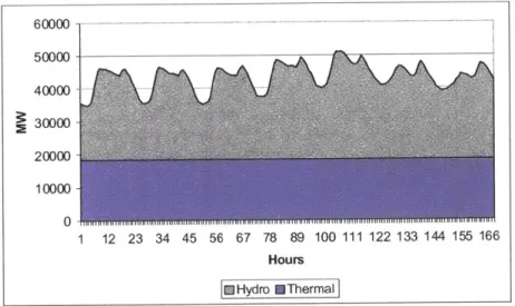
For the first scenario that was run, the results were adequate. From the graphs shown below, we see that hydro varies throughout the week and that thermal production is constant.

60000 --- -- - - 50000-30000 20000 10000 0 1 12 23 34 45 56 67 78 89 100 111 122 133 144 155 166 Hours m Hydro m Thermal

Figure 3-1: The total load divided into the parts met by hydro and thermal generation.

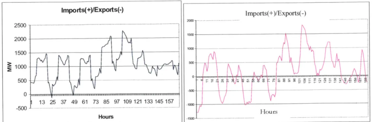
In order to gauge the accuracy of our hydro scheduling methodology, imports/exports from PROSYM are compared with actual imports/exports for that week in Norway. From the figures below, it is apparent that Norway imports during off-peak hours and exports during peak-hours which is consistent with what occurs in reality. One point to take note of is that the difference between peak imports and peak exports that PROSYM produces is approximately 4000, where as

Imports(+)IExports(-) -

1/11%

Figure 3-2: Imports/exports for Norway in week 8 using the flat thermal and varying hydro scheme. The figure on the left is the estimated imports/exports from the PROSYM model and the figure on the right is the actual exchange for Norway.

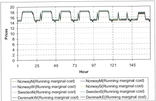
Another issue that arose is the fact that scheduling hydro in this manner is not realistic, as no hydro power is banked for future use. All available hydro power is dispatched and thermal production is flat across all hours of the week. This issue becomes more apparent as we focus on the prices in the transmission areas. In the figure below, prices in Norway North drop down.

20 ---- -- --- - -- - - - - -15 10 --- -- -- -- --- - - - - - - - - -- - ---5 -- --- - -- - - --- - - -- - - -L 0 1 25 49 73 97 121 145 Hour

-NorwayN(Running marginal cost) -NorwayM(Running marginal cost)

-NorwayW(Running marginal cost) NorwayS(Running marginal cost)

- SwedenN(Running marginal cost) - SwedenS(Running marginal cost)

- DenmarkW(Running marginal cost) -DenmarkE(Running marginal cost)

Figure 3-3: Prices in the transmission areas for week 8 estimated by PROSYM using the flat thermal and varying hydro scheme.

This is due to the fact that there is too much hydropower available in that area and all of it cannot be exported due to transmission constraints. Therefore since the power cannot be saved or stored, it simply goes to waste. In reality, system operators have knowledge of transmission line constraints and will schedule hydro in a manner that would not violate these constraints. They might choose to bank the hydro for later use when prices are high. However this scheduling

4000 3000 2000 1000 0

-methodology lacks the flexibility to allow hydro banking, as hydro power production is predetermined.

3.2.2 Flat Hydro/Varying Thermal Results

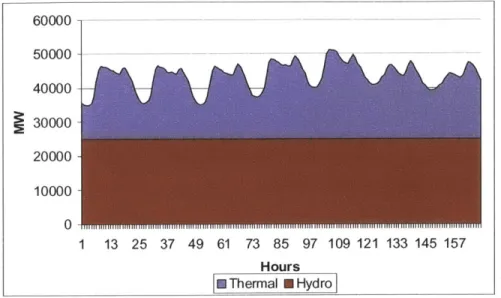
The next scenario that was run gave results that were not entirely accurate. From the graphs shown below, we see that in this scenario, hydro production is a constant throughout the week and thermal production varies from hour to hour.

60000 50000 40000 30000 20000 10000 0 1 13 25 37 49 61 73 85 97 109 121 133 145 157 Hours m Thermal U Hydro

Figure 3-4: The total load divided into the parts met by hydro and thermal generation.

Once again, looking at the imports/exports from PROSYM (below) and comparing them to actual imports/exports for that week, the PROSYM output indicates that Norway imports during peak hours and exports during off-peak hours, which is opposite of what actually occurs in reality. Another important point to take note of in this scenario is that in a system which is dominated by hydro power, it is illogical to have a flat hydro production curve. Especially in the Scandinavian case, where hydro power accounts for more than half of the energy production in the area, a varying thermal production along with a constant hydro production is unable to meet the load.

Imports(+yExports(-) Inpods(+Y/Bqorts(-) 4000 3000 2000---1000 -2000 - --201 -3000- -4000-MW AOM

Figure 3-5: Imports/exports for Norway in week 8 using the varying thermal and flat hydro scheme. The figure on the left is the estimated imports/exports from the PROSYM model and the figure on the right is the actual exchange for Norway.

3.2.3 Varying Hydro/Thermal Results

The last scenario that was run gave results that were closer to reality. This last scenario was partly derived from the first case where thermal production was flat and hydro production varied throughout the day. Since the imports/exports data for that scenario was closest to reality, the loads were adjusted using the formula below, to produce an import/export graph that was more similar to the actual.

ltnew =

1

where

itnew = new varying hydro area load

= average hydro area load over week

= hydro area load with complete load leveling C1 = load leveling factor (= 0.5)

The purpose of using the formula was to compress the graph so that that difference between peak imports and peak exports is decreased to a level that mimics reality more closely. This is done by calculating the average load over the week and multiplying the difference between the average and the actual by a load-leveling factor. This methodology gives us varying thermal and hydro production curves as shown below. The two curves follow the same pattern as they both have

higher production during peak hours and lower during off-peak hours. Comparing PROSYM import/export data to the actual data from the graphs below, we see that this new method has decreased the difference between peak imports and exports to approximately 3000.

Imports(+)/Exports(-) 2000 - - _-- -1500 1000 -500 0 -500 13 25 37 49 61 73 85 7 10 21 13 145157 -1000 Hours 4000 3000 2000 -1000 - 0 .. .. Acofo- 49515

Figure 3-6: Imports/exports for Norway in week 8 using the varying thermal and varying hydro scheme. The figure on the left is the estimated imports/exports from the PROSYM model and the figure on the right is the actual exchange for Norway.

This analysis assumes that hydro producers are behaving ideally by trying to level the load completely. However, there are several reasons as to why hydro producers may not act idealistically. For example, transmission limits may impose constraints on the manner in which hydro producers schedule production. Uncertainty in load may also lead to non-idealistic behavior as load estimates are essentially predictions as to how much power will be needed. Lastly, hydro producers may purposely act in a non-idealistic fashion by decreasing production leading to higher prices. Production is then increased at these high prices in order to maximize profits.

Looking at graphs for other areas, PROSYM import/export data for Sweden seems to be a translated version of the actual import/export graphs. The peaks and shape of the graph are very similar, however the PROSYM output indicates that Sweden is mainly an importer, where as in actuality Sweden both imports and exports. There are two possible explanations for the discrepancy in this case. First, Sweden's electricity infrastructure is composed of both thermal and hydro generation. The load-leveling factor analysis used does not take this into account. Secondly, the run-of-river content in Sweden South is a large percentage of the actual energy production from hydro. The analysis used does not differentiate between run-of-river content and actual energy production. Future iterations of the load-leveling analysis will take these issues into

2500 2000 1500 1000 500-0 -500 -Imports(+)/Exports(-) - ---Imports(+)/Exports(-) 13 25 37 49 61 73 85 97 Hours

Figure 3-7: Imports/exports for Sweden in week 8 using the varying thermal and varying hydro scheme. The figure on the left is the estimated imports/exports from the PROSYM model and the figure on the right is the actual exchange for Sweden.

Finally, examining the PROSYM import/export graphs for Denmark, there seems to be a regular pattern with high exports during off-peak hours and low exports during peak hours. Comparing the PROSYM data with actual imports/exports for Denmark, it is consistent in the fact that both describe Denmark as an exporter. However, the actual data does not have the same regular pattern as the PROSYM output. In the case of Denmark, the load-leveling methodology has no direct effect as Denmark's generation does not include hydro. However, this method may be indirectly affecting the PROSYM results for Denmark. But, as this load-leveling methodology is improved for Norway and Sweden, it may adjust the results for Denmark as well. The large fraction wind power might give "irregularities" in the actual Danish data.

Imports(+)/Exports(-) Import(+)1EkSport(-) 500-0 - ... -. -.. .. - .. 11"11.1111..11. ...- ... -7fm 1 1 13 25 37 49 61 73 85 97 109 121 133 145 157 -500- -f--l 1 ,b 0 1000 0 -1500 -1500--2000 . -2500 ---- - 2-- Hours Hours -2000 -

-Figure 3-8: Imports/exports for Denmark in week 8 using the varying thermal and varying hydro scheme. The figure on the left is the estimated imports/exports from the PROSYM model and the figure on the right is the actual exchange for Denmark.

Validity of these results can be further verified by examining the prices in the various transmission areas. As can be seen from the graph below, prices are high during peak hours and lower during off-peak hours. The prices follow a very similar pattern throughout the week, with some variation

109 121 133 145 157 I1 _Hours -- - -- --- A 1000 500 0 -500 -15WJ

in the weekend. Unlike before, where the price in Norway North fell to $3, there are no such price drops or spikes. This demonstrates that transmission constraints were not violated.

. .0 20 18 16 14 12 10 8 6 4 2 0 --- ---- - - - - -- --- --- ---1 25 49 73 97 121 145 Hour

-NorwayN(Running marginal cost) -NorwayM(Running marginal cost) -NorwayW(Running marginal cost) NorwayS(Running marginal cost)

- SwedenN(Running marginal cost) - SwedenS(Running marginal cost)

- DenmarkW(Running marginal cost) - DenmarkE(Running marginal cost)

Figure 3-9: Prices in the transmission areas for week 8 estimated by PROSYM using the flat thermal and varying hydro scheme.

Overall the results acquired from this method closely mimic reality. Using this method no transmission constraints are violated and prices are reasonable. The PROSYM import/export profile for Norway matches the actual data very closely. For Sweden and Denmark, the profiles have the correct shape and accurately describe the region as an importer/exporter, but further work is required in order to account for areas with thermal production. Also, the load-leveling method must be improved in areas for which the run-of-river content is a large part of the hydro production.

3.3 Improving the Hydro Scheduling Methodology 3.3.1 Representative Weeks

In order to continue with this analysis, a representative set of weeks from the year must be chosen in order to test the results. Although this analysis can be done for all weeks of the year, a good sample set of weeks will suffice. In order to choose these weeks, the load as well as the inflow

I

throughout the year. This was probably one of the coldest weeks in Scandinavia and would be a good week to use in testing our hydro scheduling methodology.

Load per week

8000 -- - - ---- -~~~--- --- --- --- 300000 7000 -- ₂₅₀₀₀₀ 6000 -200000 5000-4000 150000 C 00 3000- ₁₀₀₀₀₀ 2000 50000 1000 0F 0

Figure 3 -10: The aggregate load for Norway in 2001.

Week 30 was the next logical choice as it had had the lowest load throughout the year. Week 30 was a summer week with low load coupled with a high run-of-river content and moderate reservoir inflow in both Norway and Sweden, as shown by the figure below.

7000 6000 ---

-I

---I

I

I.

Week 24 was another logical choice as it represented a late spring week with high reservoir inflow and run-of-river production coupled with moderate temperatures in both Norway and Sweden.

I

* Load B ROR U Res iflow

Figure 3-12: The aggregate load for Sweden along with ROR content and reservoir inflow levels for 2001.

Thus far, weeks 6, 8, 24, and 30 were chosen. To represent a typical fall and winter week, weeks 41 and 48 were chosen, respectively. Week 41 was a typical fall week characterized by moderate load, run-of-river content, and reservoir inflow. Week 48 was a winter week characterized by high load coupled with low run-of-river content and low reservoir inflow for both Norway and Sweden. Using the weeks selected here, the hydro scheduling methodology will be fine tuned and tested for Norway, Sweden, and Denmark.

3.3.2 Results of Hydro Scheduling Methodology for Representative Weeks

Once the weeks were selected, the corresponding data had to be prepared for the analysis. Using the formula presented above, new loads were created for each of the areas for the weeks selected. These new loads were entered into PROSYM and consequently PROSYM produced import/export graphs for each of the areas. Comparing these graphs with actual exchange data shows that the factor method works well, but improvements are required. An issue that was encountered when

was often a large percentage the energy production for an area. In this case, to avoid losing the energy from the run-of-river content, much flexibility was lost in how the hydro was scheduled. In particular, Sweden South had a hydro production curve that was approximately flat for week 24 and week 30 as the run-of-river content was almost 100% of the production for that area. In this case, all hydro production came strictly from the run-of-river content and therefore was not

scheduled in a manner that took into account peak/off-peak periods.

The results for week 6 are quite similar to those of week 8 presented previously. PROSYM produces an import/export graph for Sweden which is a translated version of the actual import/exports for that area.

4000----3000 -2000 -

_I

- Norway Actual - Norway PROSYM

2500--2000_ 1500 1000 - -, 500-2 0 -500-11529 -1000 -1500 -2000 Hours

- Sweden Actual - Sweden PROSYM

For week 24 and week 30, the import/export graphs created by PROSYM are all translated versions of the actual import/exports. This translation can be attributed to the high run-of-river

content during these weeks. A correction for this will be discussed later in this chapter.

4000 -- - -- - - - -3000 2000 1000 2 0

-1oo

- Norway Actual - Norway PROSYM

4000 3000 - 2000-1000 -2

0 . . ... ... . .. .. .. .. . .

...

...

...

...

- Sweden Actual - Sweden PROSYM Figure 3-14: Actual and estimated imports/exports for both Norway and Sweden for week 24.

5000 4000. 3000_ 2000-2 1000 -0 -1000 15 29 43 5 71 85 99 13 127 141 155 -2000 --- -- --- __ ----Hours

- Norway Actual - Norway PROSYM

-500 15 29 43 57 71 85 99 113 97 141 -1000 - --1500 -2000 -S -2500 --- A-- 3000 --3500 -4000 - - - - -- - -Hours

- Sweden Actual - Sweden PROSYM Figure 3-15: Actual and estimated imports/exports for both Norway and Sweden for week 30.

I

Since the run-of-river content is still a large percentage of the energy production in week 41, the same translation phenomenon can be seen quite clearly. For week 48, the translation is less pronounced as much of the snow has melted leading to a smaller run-of-river contribution.

2000- 100010 --2000 -3000 --- - ----Hours

- Norway Actual - Norway PROSYM

-500 --1000 -1500- n -2000 2 -2500 -3000 - - - --3500 -4000 -- - --4500 -- - -Hours

- Sweden Actual - Sweden PROSYM Figure 3-16: Actual and estimated imports/exports for both Norway and Sweden for week 41.

2000- 100 0- -1000-2 -2000- -3000- -4000- -5000-Hours

- Norway Actual - Norway PROSYM

2500-2000 1500-1000 500 0--500 -1000 a...,... ... ... . ... ... " -nnfi - -S13 25 37 49 61 73 85 97 109 12113314 157 Hours

- Sweden Actual - Sweden PROSYM Figure 3-17: Actual and estimated imports/exports for both Norway and Sweden for week 48.

3.3.3 Factor Adjustment for Run-of-River Content

As presented above, when the run-of-river content is low, the hydro scheduling methodology works quite well. However, as the run-of-river content increases, the import/export graphs created by PROSYM maintain the same shape as the actual exchange data, but a translation takes place. Looking at the graphs for week 24 above, it is apparent that the PROSYM import/export graphs are a translated version of the actual exchange data. To determine the root of this behavior, the run-of-river content was analyzed for the six weeks in question. From the table below, we see that the run-of river is a small percentage of the energy production in the winter weeks except for Norway Mid and Sweden South. Proceeding through the year, we see that the run-of-river content is a much larger percentage of the energy production in the various areas. This is accurate because as

15 "T 43 7 85 11 12 17

the temperature rises, snow on the mountains melt and drain into the rivers. As the contribution from the river gets larger, the hydro scheduling methodology loses flexibility as the run-of-river content must be utilized or else it is wasted. This is a dilemma faced by hydro producers in reality because there is no control over the timing and the amount of the run-of-river content. Since it must be used and there is no control over how much comes and when, hydro producers lose much freedom in scheduling the hydro the way they wish to. Nonetheless, as can be seen from the import/export data, the hydro producers do deal with this issue in some respect. Therefore, the hydro scheduling methodology presented must account for this run-of-river situation appropriately.

Week 6 Week 8 Week 24 Week 30 Week 41 Week 48

NorwayN 1% 2% 56% 66% 33% 5% NorwayM 19% 19% 68% 82% 54% 26% NorwayW 4% 4% 61% 84% 63% 10% NorwayS 7% 6% 75% 73% 70% 17% SwedenN 2% 5% 66% 90% 86% 24% SwedenS 21% 13% 100% 99% 95% 89%

Table 3-1: The percentage of hydro that is run-of-river for the six hydro areas in our analysis.

In order to correct the hydro scheduling methodology, the factor method must somehow take into account the run-of-river content when producing the new loads. Given that the shape of the graph is correct, one must determine how to translate the graph appropriately such that it more closely mimics what occurs in reality. One such method for doing this is to adjust the new loads that are calculated by subtracting a fixed amount from them. This would essentially just translate the curve downward. The next step is calculation of this factor. Looking at the graphs closely we see that in most cases the import/export graphs produced by PROSYM are approximately 1000 above the actual import/export graphs. One possible method for adjusting the loads is to simply subtract 1000 from the load in each hour of the day. However, this method does not take into account the percentage of hydro energy that comes from the run-of-river content. A better method, one that involves the run-of-river content, is one where the amount subtracted from the new load is the percentage of hydro energy that consists of run-of-river content multiplied by 1000, as shown in the figure below.

itnew _I+= (

I

where

Anew new varying hydro area load

= average hydro area load over week

hydro area load with complete load leveling C1 = load leveling factor (= 0.5)

R

In order to use the formula above, we must aggregate the run-of-river percentages for each week for all of Norway and Sweden. Doing this gives us the run-of river percentages presented below.

Week 6 Week 8 Week 24 Week 30 Week 41 Week 48

Norway 6% 6% 68% 76% 61% 14%

Sweden 3% 6% 71% 91% 87% 30%

Table 3-2: The percentage of hydro that is run-of-river for Norway and Sweden.

3.3.4 Results of Factor Adjustment for Run-of-River Content

Using these percentages and the correct formula presented above, new loads were created and simulations were run once again. As shown below, the improved formula has taken into account the run-of-river content and PROSYM has produced import/export graphs that mimic reality. Only weeks with run-of-river percentages above 50% are presented below.