Analytical methods to interpret ground deformations due to soft ground tunneling

(1)

ANALYTICAL METHODS TO INTERPRET GROUND DEFORMATIONS DUE TO SOFT GROUND TUNNELING

by

Federico Pinto Ingeniero Civil (1997) National University of Cordoba

SUBMITTED TO THE DEPARTMENT OF CIVIL AND ENVIRONMENTAL ENGINEERING

IN PARTIAL FULFILLMENT OF THE REQUIREMENTS FOR THE DEGREE OF MASTER OF SCIENCE IN CIVIL AND ENVIRONMENTAL ENGINEERING

at the

MASSACHUSETTS INSTITUTE OF TECHNOLOGY September 1999

S ignature of A uthor...

Department of Civil and Environmental Engineering September 30, 1999

C ertified b y ... ... -.. V . v &#. . . Andrew J. Whittle Associate Professor of Civil and Environmental Engineering Thesis Supervisor

A ccep ted b y ... ... ... ... Daniele Veneziano Professor of Civil and Environmental Engineering Chairman, Departmental Graduate Committee MASSACHUSETTS INSTITUTE

OF TECHNOLOGY

MASSACHUSETTS INSTITUTE OF TECHNOLOGY

(2)

ANALYTICAL METHODS TO INTERPRET GROUND DEFORMATIONS DUE TO SOFT GROUND TUNNELING

by Federico Pinto

Submitted to the Department of Civil and Environmental Engineering on September 30, 1999, in partial fulfillment of the requirements for the degree of

Master of Science in Civil and Environmental Engineering

ABSTRACT

This thesis studies the application of simplified analytical models for predicting ground deformations caused by tunneling. The analytical models are principally based on the assumption of linear elastic ground mass response. Complete solutions are presented for ground movements in a 2-D half-plane due to prescribed deformation modes at the circular tunnel cavity wall. Preliminary 3-D solutions are also presented for the case of a tunnel heading with a uniform rate of ground convergence. The results show that approximate models based on point ground losses and distortions provide a good approximation to solutions from analyses that model the exact tunnel geometry. Further analyses show how deformations around a rectangular tunnel drift can be modeled by a series of line sinks. Deformations occurring close to the tunnel cavity are influenced by soil plasticity. The thesis proposes a simple correction factor that should be applied to measurements of cavity convergence in order to estimate far-field elastic ground movements. An alternative approach, proposed by Sagaseta (1988), assumes an average dilation rate due to plastic behavior in the soil mass. This average dilation model produces significant differences in the predicted far-field deformation pattern.

The proposed analyses have been validated using data from published case studies of tunnels constructed using different techniques and soil properties. A simple procedure is proposed for estimating the three model input parameters based on surface settlement and inclinometer data. Three of the examples show encouraging agreement with the proposed analysis. However, data from a fourth project, a deep NATM tunnel in stiff London Clay, is not consistent with either the proposed elastic or average dilation models. The proposed analysis is now available for comparison with monitoring data from the on-going Tren Urbano project in San Juan.

Thesis Supervisor: Prof. Andrew J. Whittle

(3)

ACKNOWLEDGEMENTS

I would like to thank Prof. Andrew J. Whittle for his kind support, continuous positive feedback and the energy that he dedicated towards the completion of this thesis. His insight lead me through this new and challenging experience. I would also like to thank the Tren Urbano team at MIT; Dr. John T. Germaine, Yun Kim, Guoping Zang, and Yo-Ming Hsieh, who continuously provided new ideas and insightful comments towards my work. The interaction amongst the team has made this experience very enjoyable. I would like to acknowledge the economic support provided by Tren Urbano through a contract between MIT and the KKZ/CMA Joint Venture responsible for design-build of Section 7 in Rio Piedras. The economic support provided by Fulbright/CONICOR during the summer is also gratefully acknowledged.

Acknowledgements also go out to:

Prof. Carlos A. Prato, who encouraged me to pursue graduate studies in Civil Engineering and was instrumental in nourishing my interest for research.

Prof. Hai S. Yu, who contributed to this thesis during his stay at MIT. The faculty of the Mechanics and Materials group at MIT.

Last but not least, I would like to thank my family, who has been the main source of my strength and inspiration during this challenging year. My fellow students and friends from the Geotech group at MIT; Jorge Gonzalez, Martin Nussbaumer, Alexis Liakos, Dominic Assimaki, George Kokossalakis, Christoph Haas, Attasit 'Pong' Korchaiyapruk, Dimitrios Konstantakos, Sanjay Pahuja, Catalina Marulanda, Kurt Sjoblom, Laurent Levy, Lana Aref and Kortney Adams. Their friendship is a treasure that I will carry with me forever.

(4)

(5)

TABLE OF CONTENTS Chapter Page T itle p age ... 1 Abstract... 2 Acknowledgments... . 3 Dedication... 4 Table of Contents... 5

L ist of F igu res... 9

N o tatio n ... 2 5 1. Introdu ction ... 33

1.1. T hesis O utline... 38

2. 2-D Deformation Analyses for a Deep Circular Tunnel in an Infinite Elastic Soil... 43

2.1. Uniform hydrostatic compression... 44

2.2. Pure Distortion... 48

2.3. Relative Distortion... 56

2.4. Influence of Internal Pressure Inside Tunnel... 58

3. 2-D Deformation Analyses for a Circular Tunnel in an Elastic H alf-Plane... 63 3.1. B ackground ... 63 3.2. Exact Solutions... 64 3.2.1. Uniform Convergence... 66 3.2.2. Pure Distortion... ... 68 3.3. Approximate Solutions... 71 3.3.1. Uniform Convergence... 71 3.3.2. Pure Distortion... ... 77

3.4. Comparison of Displacement Solutions for Shallow Tunnels... ... 82

3.4.1. Uniform Convergence Mode... 83

(6)

3.4.1.2. Vertical Displacements... 84

3.4.2. Pure Distortion Mode... 86

3.4.2.1. Horizontal Displacements... 86

3.4.2.2. Vertical Displacements... 88

3.4.3. Conclusions... 90

3.5. Relative D istortion... 91

3.5.1. Effects of Relative Distortion on Surface Displacements... 92

3.5.1.1. General Features... 93

3.5.1.2. Vertical Displacement at x = 0... 94

3.5.1.3. Maximum Horizontal Displacement... 95

3.5.1.4. Width of the Settlement Trough... 96

3.5.2. Effects of Relative Distortion on Horizontal Displacements on a Vertical Line Inside the Ground... 97

4. Influence of Tunnel Geometry. Rectangular Drift... 149

4.1. Green Functions for the Displacements due to a Cavity Contraction/Expansion in an Elastic H alf-Plane... 149

4.2. Displacement Field due to Uniformly Distributed Ground Loss Along a Rectangular Line... 151

4.3. Comparison of Displacement Solutions... 152

4.4. C onclusions... 153

5. Influence of Soil Plasticity... 167

5.1. 2D Deformation Analyses for a Deep Circular Tunnel in an Infinite Soil... 167

5.1.1. Undrained Plastic Deformations due to a Cylindrical Cavity Contraction... 167

5.1.2. Drained Deformations due to a Cylindrical Cavity Contraction... 168

(7)

5.2. Approximation of Dilation Effects for a Shallow Tunnel... 173

5.3. C onclusions... 176

6. Comparison With Field Monitoring Data... 193

6.1. Design Charts for Estimating Model Input Parameters... 193

6.2. C ase Studies... 194

6.1. Case 1: Metro de Madrid (Sagaseta et al., 1999) ... 195

6.2 Case 2: Sewer-Line Tunnel in Mexico City (Romo, 1997)... 197

6.3. Case 3: Heathrow Express Trial Tunnel (Deane and Basset, 1995)... 199

6.4. Case 4: N-2 Contract for the San Francisco Clean Water Project (Clough et al., 1983)... 202

7. 3-D Effects. Semi-Infinite Tunnel... 240

7.1 3-D Deformation Analysis due to a Cavity Contraction/Expansion in Elastic Infinite Space... 240

7.2. 3-D Deformation Analysis due to a Cavity Contraction/Expansion in Elastic Half Space... 242

7.3. 3-D Deformation Analysis due to a Semi-Infinite Tunnel in Elastic Half-Space... 249

7.4. C onclusions... 254

8. Summary, Conclusions, and Further Recommendations... 261

8.1. Sum m ary ... 26 1 8.2. Modeling Considerations... 262 8.3. Further Recommendations... 263 R eferences... 265 A ppend ix I... 2 69 A ppend ix II... 27 9 A ppendix III... 289 A ppendix IV ... 293 A ppendix V ... 30 1

(8)

(9)

LIST OF FIGURES

Figure

1.1. Surface settlements predicted by Peck's empirical approach

1.2. Inflection point as a function of soil type and embedment ratios H/2R

1.3. Point cavity contraction, after Sagaseta, 1986

2. 1. Initial state of stresses

2.2. Boundary conditions at infinity

2.3. Displacements pattern at the tunnel wall

2.4. Effect of ground state on relative distortion

2.5. Effect of internal pressure on relative distortion

3.1. Problem outline

3.2. Basic deforming modes for tunnel wall (after Sagaseta, 1999)

3.3. Conformal mapping (after Verruijt, 1997)

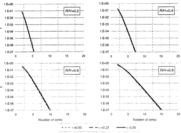
3.4. Uniform Convergence, definition of uE

3.5. Number of series terms needed for accurate evaluation of the Goursat functions

3.6. Corrections for analytic solutions using functions of complex variables

Page 40 40 41 60 60 61 61 62 98 98 99 99 100 100

(10)

3.7. Springs constants along tunnel wall, R/H = 0.5 (Verruijt, 1997)

3.8. Tunnel wall deformations for conbined uniform convergence and vertical translation, ue/R = 0.4

3.9. Surface displacements for uniform convergence, R/H = 0.5, v= 0.25

3.10. Normalized ground displacements, RIH = 0.5, v= 0.25

3.11. Convention for tunnel distortion

3.12. Complex vector decomposition

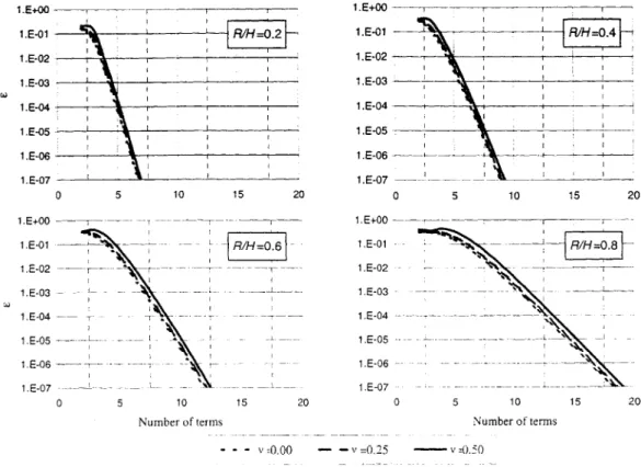
3.13. Fourier coefficients (equation {3-19})

3.14. Number of terms needed for evaluation of the Goursat functions

3.15. Vertical translation correction for tunnel wall radial distortion case

3.16. Tunnel wall deformations for combined pure distortion and vertical translation, u3/R = 0.4

3.17. Surface displacements, R/H = 0.5, v= 0.25

3.18. Ground deformations, R/H = 0.5, v= 0.25

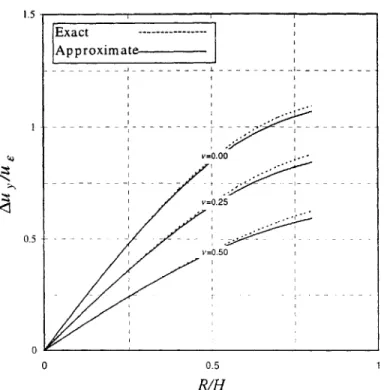
3.19. Outline of solution method proposed by Sagaseta (1987)

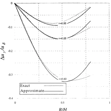
3.20. Vertical translation of tunnel springline for approximate solution for uniform convergence mode

101 102 102 103 103 104 104 105 105 106 106 107 107 108

(11)

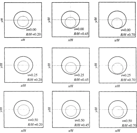
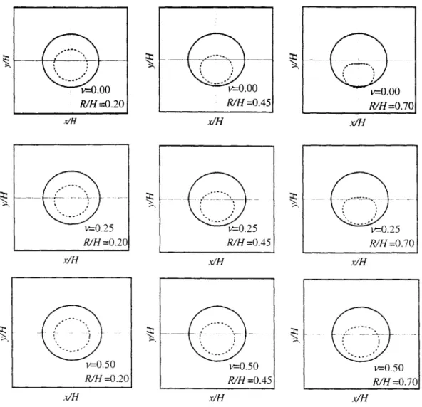
3.21. Deformations of tunnel wall due to uniform convergence mode with uE/R=-0.4 by approximate method

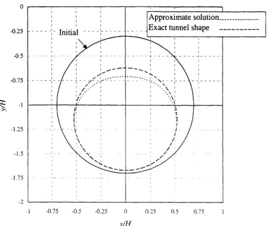
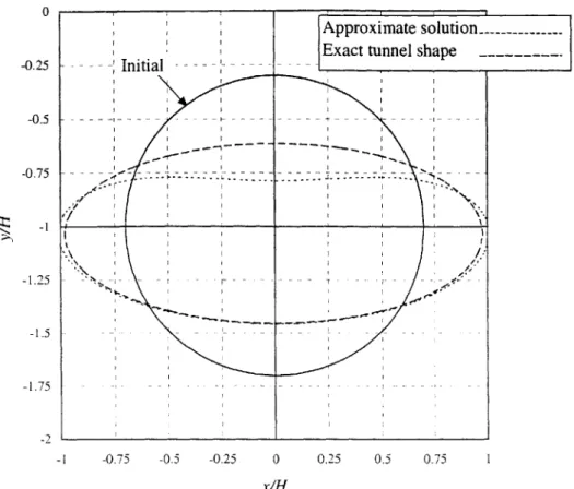
3.22. Effects of approximation of tunnel shape on deformed tunnel wall with u,/R=-0.4, R/H = 0.7, v= 0.25

3.23. Normalized surface displacements. R/H = 0.5, v= 0.25

3.24. Normalized ground displacements. R/H = 0.5, v= 0.25

3.25. Volume of expansion due to pure distortion

3.26. Vertical translation of tunnel springline from approximate solution for pure distortion mode

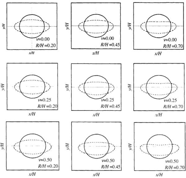
3.27. Deformations of tunnel wall due to pure distortion with u6/R = 0.4

by approximate method

3.28. Effect of approximation of tunnel shape on deformed tunnel wall

for uE/R = -0.4, R/H = 0.7, v = 0.25

3.29. Normalized surface displacements for pure distortion mode. Approximate solution for R/H = 0.5, v= 0.25

3.30. Normalized ground displacements for pure distortion mode. Approximate solution for RIH = 0.5, v= 0.25

3.31. Critical R/H ratio vs. Poisson ratio

3.32. Surface displacements due to uniform convergence mode, R/H = 0.20, v = 0.00 109 110 110 111 111 112 113 114 114 115 115 116

(12)

3.33. Ground displacements due to uniform convergence mode, RIH = 0.20, v= 0.00

3.34. Surface displacements due to uniform convergence mode, R/H = 0.20, v = 0.25

3.35. Ground displacements due to uniform convergence

mode, R/H = 0.20, v= 0.25

3.36. Surface displacements due to uniform convergence mode, R/H = 0.20, v= 0.50

3.37. Ground displacements due to uniform convergence mode, R/H = 0.20, v= 0.50

3.38. Surface displacements due to uniform convergence mode, R/H = 0.45, v= 0.00

3.40. Surface displacements due to uniform convergence mode, R/H = 0.45, v= 0.25

3.42. Surface displacements due to uniform convergence mode, R/H = 0.45, v= 0.50 116 117 117 118 118 119 119 120 120 121

(13)

3.43. Ground displacements due to uniform convergence mode, R/H = 0.45, v= 0.50

3.45. Ground displacements due to uniform convergence mode, R/H = 0.70, v= 0.00

3.50. Surface displacements due to pure distortion

mode, R/H = 0.20, v= 0.00

3.51. Ground displacements due to pure distortion mode, R/H = 0.20, v= 0.00

3.52. Surface displacements due to pure distortion mode, R/H = 0.20, v= 0.25 121 122 122 123 123 124 124 125 125 126

(14)

3.54. Surface displacements due to pure distortion mode, R/H = 0.20, v = 0.50

3.55. Ground displacements due to pure distortion

mode, R/H = 0.20, v= 0.50

3.56. Surface displacements due to pure distortion mode, RIH = 0.45, v= 0.00

mode, R/H = 0.45. v= 0.00

3.58. Surface displacements due to pure distortion

mode, R/H = 0.45. v= 0.25

mode, R/H = 0.45, v= 0.25

3.60. Surface displacements due to pure distortion mode, RIH = 0.45, v= 0.50

3.62. Surface displacements due to pure distortion mode, R/H = 0.70, v= 0.00 126 127 127 128 128 129 129 130 130 131

(15)

3.64. Surface displacements due to pure distortion mode, R/H = 0.70, v= 0.25

3.65. Ground displacements due to pure distortion mode, R/H = 0.70, v= 0.25

3.66. Surface displacements due to pure distortion mode, R/H = 0.70, v= 0.50

3.67. Ground displacements due to pure distortion mode, R/H = 0.70, v= 0.50 3.68. Surface displacements, R/H = 0.20, p = -0.5, v= 0.25 3.69. Ground displacements, R/H = 0.20, p = -0.5, v= 0.25 3.70. Surface displacements, R/H = 0.20, p = 0.5, v= 0.25 3.71. Ground displacements, R/H = 0.20, p = 0.5, v = 0.25 3.72. Surface displacements, R/H = 0.20, p = 1, v= 0.25 3.73. Ground displacements, R/H = 0.20, p = 1, v= 0.25 3.74. Surface displacements, R/H = 0.45, p = -0.5, v= 0.25 3.75. Ground displacements, R/H = 0.45, p = -0.5, v= 0.25 131 132 132 133 133 134 134 135 135 136 136 137 137

(16)

3.76. Surface displacements, R/H = 0.45, p = 0.5, v= 0.25 3.77. Ground displacements, R/H = 0.45, p= 0.5, v= 0.25 3.78. Surface displacements, R/H = 0.45, p = 1, v= 0.25 3.79. Ground displacements, R/H = 0.45, p = 1, v= 0.25 3.80. Surface displacements, R/H = 0.70, p = -0.5, v= 0.25 3.81. Ground displacements, R/H = 0.70, p = -0.5, v= 0.25 3.82. Surface displacements, R/H = 0.70, p = 0.5, v= 0.25 3.83. Ground displacements, R/H = 0.70, p = 0.5, v= 0.25 3.84. Surface displacements, R/H = 0.70, p = 1, v= 0.25 3.85. Ground displacements, R/H = 0.70, p = 1, v= 0.25

3.86. Influence of v on the normalized surface vertical

displacement at x = 0, p = 0.5

3.87. Influence of p on the normalized surface vertical displacement at x = 0, v= 0.25

3.88. Influence of relative distortion on the location of maximum horizontal displacement

138 138 139 139 140 140 141 141 142 142 143 143 144

(17)

3.89. Influence of relative distortion on the normalized maximum horizontal displacement

3.90. Influence of embedment ratio, R/H, on the surface settlement distribution. p=0.5; v= 0.25

3.91. Influence of Poisson ratio, v, on the surface settlement distribution. p=1; R/H = 0.45

3.92. Influence of relative distortion, p, on the surface settlement distribution for v= 0.25 ; R/H = 0.45

3.93. Horizontal displacement distribution, p = 1.0

3.94. Horizontal displacement distribution, v= 0.25

3.95. Horizontal displacements at x = 2-R, p = 1, v = 0.25

3.96. Horizontal displacements at x = 2-R, p = 1, R/H = 0.5

3.97. Horizontal displacements at x = 2-R, v= 0.25, R/H = 0.5

4.1. Arbitrary cavity contraction

4.2. Modeling of distributed ground loss along rectangular drift

4.3. Surface displacements due to uniformly distributed ground loss

along rectangular tunnel for D/B = 1, D/2H=0.2, and v=0.25

144 145 145 146 146 147 147 148 148 155 155 159

(18)

4.4. Ground displacements due to uniformly distributed ground loss

along rectangular tunnel for DIB = 1, D/2H=0.2, and v =0.25

along rectangular tunnel for DIB = 1, D/2H=0.45, and v = 0.25

4.6. Ground

4.7. Surface

displacements due to uniformly distributed ground loss

along rectangular tunnel for DIB = 1, D/2H=0.4, and v = 0.25

displacements due to uniformly distributed ground loss

along rectangular tunnel for D/B = 1, D/2H=0.7, and v= 0.25

along rectangular tunnel for DIB = 1, D/2H=0.7, and v = 0.25

along rectangular tunnel for BID = 0.5, D/2H = 0.45, and v= 0.25

4.10. Ground displacements due to uniformly distributed ground loss

along rectangular tunnel for BID = 0.5, D/2H = 0.45, and v=0.25

4.11. Surface displacements due to uniformly distributed ground loss

along rectangular tunnel for BID = 2, D/2H = 0.45, and v =0.25

along rectangular tunnel for BID = 2, D/2H = 0.45, and v=0.25

4.13. Influence of embedment ratio, D/2H, on the settlement trough for v= 0.25, B/D= 1 159 160 160 161 161 162 162 163 163 164

(19)

4.14. Influence of aspect ratio, BID, on the settlement trough for v= 0.25, D/2H = 0.45

4.15. Influence of the embedment ratio, D/2H, on the horizontal

displacements at x = 2Req for v= 0.25, BID = 1

4.16. Influence of the aspect ratio, BID, on the horizontal displacements

at x = 2Re, for v = 0.25, B/D= 1

5.1. Radial displacements due to a cylindrical cavity contraction (after Yu and Rowe, 1998)

5.2. Relationship between cohesion intercept, c', and preconsolidation pressure, a'p (Mesri and Abdel-Ghaffar, 1993)

5.3. Influence of soil properties on the radius of the plastic

zone, R,, for c'/p'o = 0.0

5.4. Influence of soil properties on the radius of the plastic

zone, R,, for c'/p'o = 0.1

5.5. Influence of soil properties on the radius of the plastic zone, R,, for c'p'o = 0.2

5.6. Influence of soil properties on the radius of the plastic zone, R,, for c'/p'o = 0.3

zone, R,, for c'p'o = 0.4

164 165 166 178 178 179 180 181 182 183

(20)

zone, R,, for c'/p'o = 0.5

5.9. Influence of soil properties on the reduction factor, RF, for c'/p'o = 0.0

5.11. Influence of soil properties on the reduction factor, RF, for c'/p'o = 0.2

5.13. Influence of soil properties on the reduction factor, RF, for c'/p'o = 0.4

5.14. Influence of soil properties on the reduction factor, RF, for c'/p'o = 0.5

5.15. Influence of a on surface settlements distribution, R/H = 0.2. p = 0

5.16. Influence of a on surface settlements distribution, R/H = 0.2, p = 1

5.17. Influence of a on horizontal displacements

inside the ground, R/H = 0.2, p = 0

5.18. Influence of a on horizontal displacements

inside the ground, R/H = 0.2, p = 1

6.1. Definition of the input parameters for the proposed design charts

6.2. Case 1: Madrid Metro -Measured surface settlements

6.3. Case 1: Madrid Metro -Measured horizontal displacements at x = -8 m

184 185 186 187 188 189 190 191 191 192 192 204 205 205

(21)

6.4. Case 1: Madrid Metro -Derivation of parameters p, v

6.5. Case 1: Madrid Metro -Derivation of parameters p, v

6.6. Case 1: Madrid Metro -Derivation of parameter uy0/ue

6.7. Case 1: Madrid Metro -Derivation of parameter uy0/ue

6.8. Case 1: Madrid Metro -Surface settlements

6.9. Case 1: Madrid Metro -Horizontal displacements

6.10. Case 1: Madrid Metro -Contours of predicted ground displacements

6.11. Case 2: Sewer-line tunnel in Mexico City - Measured surface settlements

6.12. Case 2: Sewer-line tunnel in Mexico City - Measured horizontal displacements

6.13. Case 2: Sewer-line tunnel in Mexico City - Derivation of parameters p, v

6.14. Case 2: Sewer-line tunnel in Mexico City - Derivation of parameters p, v

6.15. Case 2: Sewer-line tunnel in Mexico City - Derivation of parameter uy0/ue

6.16. Case 2: Sewer-line tunnel in Mexico City - Derivation of parameter uv/ue

6.17. Case 2: Sewer-line tunnel in Mexico City - Vertical displacements

6.18. Case 2: Sewer-line tunnel in Mexico City - Horizontal displacements

206 207 208 209 210 210 211 211 212 213 214 215 216 217 218

(22)

6.19. Case 2: Sewer-line tunnel in Mexico City - Contours of predicted ground displacements (based on fit to reported data)

6.20. Case 2: Sewer-line tunnel in Mexico City - Contours of predicted ground displacements (based on fit to adjusted data)

6.21. Case 2: Heathrow Express Trial Tunnel- Soil Profile

6.22. Case 2: Heathrow Express Trial Tunnel- Cross section and excavation sequence (Type three)

6.23. Case 3: Heathrow Express Trial Tunnel - Measured surface settlements

6.24. Case 3: Heathrow Express Trial Tunnel - Measured horizontal displacements

6.25. Case 3: Heathrow Express Trial Tunnel - Derivation of parameters p, v

6.26. Case 3: Heathrow Express Trial Tunnel - Derivation of parameters p, v

6.27. Case 3: Heathrow Express Trial Tunnel - Derivation of parameter uyo/ue

6.28. Case 3: Heathrow Express Trial Tunnel - Derivation of parameter uy0/ue

6.31. Case 3: Heathrow Express Trial Tunnel - Surface settlements, criterion I

218 219 219 220 220 221 222 223 224 225 226 227 228

(23)

6.32. Case 3: Heathrow Express Trial Tunnel - Horizontal displacements at

x = -9 m, criterion 1

6.33. Case 3: Heathrow Express Trial Tunnel - Surface settlements, criterion 2

6.34. Case 3: Heathrow Express Trial Tunnel - Horizontal displacements at

x = -9 m, criterion 2

6.35. Case 3: Heathrow Express Trial Tunnel - Contours of ground

displacements predicted by criteria 1, 19-May-92

6.36. Case 3: Heathrow Express Trial Tunnel - Contours of ground displacements predicted by criteria 1, 25-May-92

6.37. Case 3: Heathrow Express Trial Tunnel - Contours of ground displacements predicted by criteria 1, 29-May-92

6.38. Vertical and horizontal sub-surface displacements in the vicinity of tunnels in London Clay (after Mair and Taylor, 1992)

6.39. Case 4: N-2 Contract tunnel - Cross section

6.40. Case 4: N-2 Contract tunnel -Measured surface settlements

6.41. Case 4: N-2 Contract tunnel -Horizontal displacements at x = -3.6 m

6.42. Case 4: N-2 Contract tunnel - Derivation of the parameters p, v

6.43. Case 4: N-2 Contract tunnel - Derivation of the parameters p, v

6.44. Case 4: N-2 Contract tunnel - Derivation of the parameter uy/us

228 229 229 230 230 231 231 232 233 233 234 235 236

(24)

6.45. Case 4: N-2 Contract tunnel - Derivation of the parameter uy0/ue

6.46. Case 4: N-2 Contract tunnel -Surface settlements

6.47. Case 4: N-2 Contract tunnel -Horizontal displacements at x = -3.6 m

6.48. Case 4: N-2 Contract tunnel. Contours of predicted ground displacements

7.1. Spherical cavity contraction in infinite space -Problem outline

7.2. Spherical cavity contraction in half space

7.3. Spherical cavity contraction along tunnel axis in half space - Green function

7.4. Modeling of semi-infinite tunnel - Distributed ground loss

7.5. Contours of normalized lateral displacement, ux/ue, for R/H = 0.2, v= 0.25

7.6. Deformed ground surface for RIH = 0.2, v= 0.25

7.7. Influence of proximity to tunnel heading on surface settlements for R/H = 0.2, v=0.25

7.8. Influence of proximity to tunnel heading on lateral displacements at x = 2-R for R/H = 0.2,v = 0.25

7.9. Influence of proximity to tunnel heading on longitudinal displacements at x = 2-R for R/H = 0.2,v = 0.25 237 238 238 239 256 256 257 257 258 258 259 259 260

(25)

NOTATION

Chapter 1

Vf Deformed volume of tunnel

V0 Initial volume of tunnel

V L Ground loss volume

u" max Maximum surface settlement

R Tunnel radius

H Depth to centerline of tunnel

x1 Inflection point of Gaussian curve

Ko Coefficient of earth pressures at rest

x, Horizontal coordinate

y Vertical coordinate

Chapter 2

R Tunnel radius

J'yo In-situ vertical effective stress Ko Coefficient of earth pressures at rest

'oh0 In-situ horizontal effective stress

Effective stress Total stress

uW In-situ pore pressures

PO In-situ average total stress

qo In-situ deviatoric stress

M One dimensional elastic modulus

Elastic constant

us Horizontal displacement

u1, Vertical displacement

(26)

y V G Ur r a,. 00 A, B, C, D us 0 EC 0 F n Q1, Q2, gl, q2 us us* p p* pr r,5 P OCR Tunnel radius

Depth to centerline of tunnel Vertical coordinate

Poisson ratio

Elastic shear modulus Radial displacement

Radial distance from tunnel centerline Radial stress

Hoop stress

Integration constants

Uniform radial convergence at the tunnel wall Uniform radial displacement parameter Angular coordinate

Shear stress

Airy's stress function

Radial variation of Airy's stress function Coefficient

Auxiliary functions Distortion displacement Ovalization parameter

Apparent distortion displacement Relative distortion

Pore pressure ratio

Apparent relative distortion Internal pressure inside tunnel Internal pressure ratio

Overconsolidation ratio

Chapter 3

R H

(27)

Ko V G Uz Ic Ut y kaj ic d 6 Ak Us

Coefficient of earth pressures at rest Poisson ratio

Goursat Functions Elastic shear modulus

Complex displacement vector Complex coordinate vector Elastic constant Horizontal displacement Imaginary constant Vertical displacement Horizontal coordinate Vertical coordinate

Mapped complex coordinate Embedment ratio parameter

Subscript

Laurent series coefficients

Arbitrary index for Laurent series coefficient Mapped coordinate at the surface

Mapped angular coordinate Fourier expansion coefficient

Uniform radial convergence at the tunnel wall Error norm

Surface vertical displacement in the far field Surface horizontal displacement in the far field Integration interval to define error norm Vertical translation

Angular coordinate in the z plane Distortion displacement

Shear tractions

Radial coordinate from tunnel centerline

U,

L

Au, #,

(28)

VL F ZXY a) QI, Q2, q, q2 W1 W2 Rc .(2 r,, r, OCR 0 U', MILX ux (v=O

Ground loss volume Airy's stress function

Fourier transform of the corrective shear tractions at the surface Auxiliary variable

Auxiliary functions

Volume expansion at the tunnel springline Volume contraction at the tunnel crown Distortion parameter

Vertical coordinate of the center of the circular area where heaving occurs

Radius of circular area where heaving occurs Area of settlement trough

Pore pressure ratio Internal pressure ratio Overconsolidation ratio

Vertical surface settlement above the crown Maximum horizontal displacement

Location of maximum horizontal displacement at the surface Horizontal displacement at the surface

Chapter 4 Ko H VL x y U fg

Coefficient of earth pressures at rest Depth to centerline of tunnel

Volume of ground loss Horizontal coordinate Vertical coordinate Horizontal displacement Vertical displacement

Functions that govern the spatial distribution of displacements due to a cavity contraction

(29)

T;, Y Green functions due to a cavity contraction

X, Y Vertical and horizontal coordinates of the point cavity

s Parametric coordinate

e(s) Local thickness of the cavity

a, b, c, d Geometric coordinates of the drift

/C Elastic constant

B Width of rectangular drift

D Height of rectangular drift

Req Equivalent radius of the drift

Chapter 5

Ko Coefficient of earth pressures at rest

Dilation angle

R, Radius of the plastic zone

u Equivalent elastic displacement at the tunnel wall

u8" Critical yield displacement at the tunnel wall

R Tunnel radius

No Flow factor

p'

Drained friction angle

Y Mohr-Coulomb parameter that depends on cohesion

c' Drained cohesion intercept

G Pre-yield average shear modulus

p'o In-situ effective stress

u4 Plastic displacement at the tunnel wall

T Function of the internal pressure

Coefficient that depends on the dilation angle

VL Ground loss volume

OCR Overconsolidation ratio

RF Reduction factor

(30)

uX Horizontal displacement

u, Vertical displacement

a Dilation parameter

usc Uniform convergence displacement

H Depth to centerline of tunnel

u,5 Distortion displacement

Appendix I

F Airy's stress function

x Horizontal coordinate

z Complex coordinate vector

p,

y, Goursat Functions

G Elastic shear modulus

uX Horizontal displacement

uv Vertical displacement

u, Complex displacement vector

Imaginary constant

c Elastic constant

Total normal stress in the horizontal direction Total normal stress in the vertical direction Shear stress

Integral of tractions along tunnel wall

Traction along tunnel wall in the horizontal direction tv Traction along tunnel wall in the vertical direction

s Parametric coordinate along tunnel boundary

C Integration constant

Mapped complex coordinate

(31)

a

R i

ai, bi, ci, d,

6 k Ak Appendix III x y F Cxy S A, B,C, D

Embedment ratio parameter Tunnel radius

Subscript

Laurent series coefficients

Mapped coordinate at the surface Mapped angular coordinate

Arbitrary index for Laurent series coefficient Fourier expansion coefficient

Horizontal coordinate Vertical coordinate Airy's stress function

Fourier transform of Airy's stress function

Fourier transform of the normal stresses at the surface Fourier transform of the shear stresses at the surface Auxiliary variable Auxiliary parameter Integration constant Appendix IV Ko (Tyr r pi p '0 R

Coefficient of earth pressures at rest Effective radial stress

Effective hoop stress

Radial coordinate from the center of the cavity Effective pressure inside cavity

In situ effective stress Radius of the cavity

(32)

Ur M A, B, C, D, J V G N, Y C R, T p Er uE Y Radial displacement

One dimensional elastic modulus Elastic constant

Integration constants Poisson ratio

Pre-yield average shear modulus Flow factor

Drained friction angle Cohesion ratio

Drained cohesion intercept Radius of the plastic zone Function of the internal pressure Plastic radial strain

Plastic hoop strain

Coefficient that depends on the dilation angle Dilation angle

Plastic displacement at the tunnel wall Critical yield displacement at the tunnel wall

(33)

1. Introduction

The steadily growing demand of modem society for public transportation systems in congested urban areas has encouraged innovations in underground construction techniques. Due to the fact that soft ground conditions are found in many of these urban areas, soft-ground excavation techniques have experienced a particularly remarkable advance. In the past fifty years the number of soft-ground tunnels has steadily increased, primarily due to the technological advance in tunnel machinery, grouting techniques and groundwater flow control. It is believed that this trend will continue to grow in the future since underground construction provides a solution for the need of space in densely populated urban areas. The technological advance has made possible the successful excavation of tunnels in a wide range of soils, under different groundwater conditions (Peck, 1969).

Section 7 of the Tren Urbano alignment in San Juan de PR is being constructed underground over a total length of 1.5 km trough the town of Rio Piedras (extending from Villa Nevarez to Hato Rey). The tunnel passes trough deep alluvial deposits of interbedded stiff clays and sandy clays, referred to as the Hato Rey fromation (often referred to as 'old alluvium'). Three construction methods are being used in order to excavate the tunnel; i) New Austrian Tunneling Method (NATM), for the alignment south of Calle Georgetti ; ii) stacked drift construction to support the excavation of the main cavern of the Rio Piedras station using a series of 15 drifts; and iii) twin bored tunnels excavated by means of a Earth Pressure Balance (EPB) Tunneling Boring Machine (TBM) from the Rio Piedras station towards the University of PR (UPR) station. The entire underground alignment is built underneath existing buildings (mainly masonry structures) and other facilities sensitive to ground deformations. Hence, ground deformations produced by the excavation activities are of great concern.

Ground deformations arise due to the fact that the initial state of stresses is altered by the excavation, generating a new state of equilibrium and mobilizing the shear strength of the soil in the near field around the excavated cavity. This strength mobilization leads to deformations at the excavation face, which cause the volume of the excavated soil, Vo, to be larger than the volume occupied by the tunnel, V. This difference between the excavated volume and the

(34)

volume occupied by the tunnel is called "ground loss", VL = Vf - Vo, and is often expressed as a ground loss ratio, VL = (Vf -Vo)/ Vo. -100 %. As the ground loss is a function of the amount of

deformations at the tunnel face, its value is inextricably linked to the construction method. Hence, the prediction of ground deformations has to somehow take into account the effects of the

construction method.

The methods of modeling ground deformations due to tunneling, range in complexity; from purely empirical results (e.g., Peck, 1969) to complex non-linear 3-D finite element analyses (e.g., Lee and Rowe, 1990).

Empirical methods

Empirical methods have the obvious advantage that they fit a certain amount of case studies and are relatively simple to use. Peck (1969) proposed an analysis method for estimating ground deformations induced by tunneling based on data (mainly from the Chicago Subway) from 18 tunnels excavated in cohesive and granular soils by means of shields or hand mined. Although the method has no theoretical basis, it has been widely adopted in engineering practice. Many case studies have been analyzed by this approach in the past 30 years (e.g., Attewell and Farmer, 1974; Oteo and Sagaseta, 1996, Bowers et al., 1996). Peck's approach characterizes the distribution of surface settlements using a Gaussian distribution curve (Figure 1.1). There are two parameters that define a particular curve; i) the surface settlement above the crown, u" and ii) the inflection point xi. These parameters were obtained for several case studies by means of matching Gaussian curves to measured surface settlements. By then correlating these parameters with geometric characteristics for each tunnel, design charts were developed for predicting ground displacements due to tunneling. The settlement at the inflection point (for the Gaussian distribution curve) coresponds to 0.61-u,"' (Figure 1.1). Hence, the inflection point was defined as the abscissa at which the observed settlement is 0.61 times the maximum. The inflection point, normalized by the tunnel radius', R, was then correlated with the embedment depth ratio, H / 2-R, to form a chart such as Figure 1.2, where the dotted lines delineate different

(35)

soil types. Since Peck's original work, more data has been included in such charts (e.g., Oteo and Sagaseta, 1996). This method, also assumes that the over-excavated volume V = Vf - Vo (i.e., ground loss) had the same magnitude than the volume of the settlement trough (i.e., the area enclosed by the original and deformed ground surface). However, it will be shown in this work (also Verruijt and Booker, 1996), that the over-excavated volume coincides with the volume of the settlement trough only if the material is incompressible2 (e.g., undrained behavior of clays). Once the inflection point and the volume of ground loss per unit length, V, are known, the maximum displacement at the surface can be evaluated by matching the volume of ground loss with the area of the settlement trough. The volume of ground loss in this approach is left unknown and is calculated by means of assuming empirical values for u,"". This method has the disadvantage that it cannot take into account complex construction activities (e.g. compensation grouting) and produces only one displacement pattern that can only be scaled by means of the inflection point, xi. Another disadvantage is that it does not predict either vertical or horizontal displacements within the soil mass3_{. However, this method has been able to mach many case} studies since the practitioner has the option of shifting the width of the trough by means of the inflection point as needed in order to match each particular case.

Finite Element Models

Finite Element models provide the most general framework for analyses of ground deformation due to tunneling. Different soil models can be incorporated in the analysis (e.g., Oettl et al., 1998), thus improving the modeling of real soil behavior. 3-D Construction activities and tunnel geometries can also be included in the analysis (e.g., Lee and Rowe, 1992). FEM models can also analyze staged construction, such as NATM (e.g., Dasari et al., 1996), EPB tunnel-soil-tunnel interactions (Bernat et al., 1999) and ground treatment, such as compensation grouting (e.g., Kovacevic et al., 1996). In order to perform such analyses the soil properties at the site (stiffness, strength, permeability, etc.) must be obtained by means of a comprehensive

1It will be shown in this work that the parameter that normalizes the spatial coordinates (i.e., x and v) is the depth to centerline, H, rather than the tunnel radius, R. If R is used in order to normalize x and v, the R/H ratio effect needs to be taken into account separately.

2 If the behavior is drained, the volume at the surface could be either larger or smaller, depending on Poisson ratio and dilation angle.

(36)

laboratory-testing program, which sometimes is not readily available. Ground water conditions (hydrostatic, steady state or transient seepage, etc.) also need to be included in the analysis, which requires sophisticated site investigation (e.g., piezometers and observation wells). The construction sequences-sometimes very complex or not known in advance-also influence on the model predictions. One advantage of these methods is that they are 'complete' in the sense that it is possible to estimate all the input parameters. Another advantage is that, by means of FEM, it is possible to model details of the tunneling process. However, the set up of the model is very time-consuming and, in many cases, the actual 3-D problem must be analyzed by 2-D

approaches in order to simplify the model. Model predictions are also highly dependent on the constitutive model assumed in order to approximate the real soil behavior.

Analytical models

These methods make gross approximations to the real soil behavior but otherwise fulfill all other axioms of continuum mechanics. Analytical methods can predict ground displacements throughout the soil mass with a very few input parameters. Moreover, the input parameters needed for the analysis are relatively simple to estimate, for which these methods are very useful in preliminary design. Most of these methods are readily extendable to 3-D and can predict both vertical and horizontal displacements throughout the soil mass. Another advantage is that they provide a framework for studying complex construction procedures, such as the stacked drift construction of the Rio Piedras cavern by direct superposition of solutions. Grouting activities can also be taken into account by assuming cavity expansions, rather than contractions. In situ Ko conditions, soil-lining interaction and construction procedure effects can also be conceptually taken into account by shifting the relative contribution of basic deforming modes at the tunnel wall. However, one major drawback of these methods is that they can not model the soil-structure interaction of pre-existing soil-structures at the surface, which in some cases may lead to large differences in ground deformations due to local yielding effects. These models may also

miss some features associated with complex soil behavior.

Sagaseta (1987) proposed simplified analytical expressions for evaluating short-term ground displacements around tunnels in clays. His solution considered a point cavity contraction (which

(37)

represented concentrated ground loss at the tunnel axis) from an initial isotropic state of stresses (i.e., Ko = 1) in an elastic half-plane (Figure 1.3). The settlement trough, evaluated by means of this solution, has a similar shape as the Gaussian distribution curve proposed by Peck (1969).

However, the resulting settlement trough is wider than the empirical distribution proposed by Peck (see Schmidt, 1988). Verruijt and Booker (1996) extended the method for arbitrary Poisson ratios and included a second deformation mode of the tunnel wall corresponding to an elastic cavity distortion from an anisotropic initial state of stresses (i.e., Ko # 1). It was found that the deformation at the tunnel wall has a significant impact on the displacement distribution at the surface and inside the ground. The distortion mode reduces the width of the settlement trough due to the isotropic compression alone. Thus, by combining both deformation modes, different displacement patterns can be modeled. The aforementioned methods do not explicitly consider the geometry of the tunnel wall in the analysis. In that sense, they are regarded as "point solutions". Verruijt (1997) presented a more refined solution method by explicitly considering the presence of the tunnel wall. His published results are limited to the isotropic case. Other approaches have been pursued by Sagaseta (1999), who modified the point solutions in order to account for dilation due to the drained shearing. The effect of the dilation is to reduce the width of the settlement trough for cavity contraction4. In practice, however, dilation is only likely to occur in the near field aaround the tunnel (where soil yields). Thus, the selection of a single dilation parameter represents a practical limitation of this approach.

Longanathan and Poulos (1998) proposed an empirical extension of the analytical solutions5 proposed by Verruijt and Booker (1996) neglecting the distortion component due to Ko # 1. Their

analysis recognizes that settlement troughs are generally wider than experimental measurements and assumes that Verruijt's solution accounted for a uniform convergence at the tunnel wall6.

Hence, the solution was modified by arbitrary functions in order to match a set of case studies and account for non-uniform displacements at the tunnel wall (larger at the crown and smaller at the invert). Although based on correct concepts, this method has no theoretical justification and

4 Dilation has the opposite effect if a cavity expansion is considered

5 Their appproach ignores the distortion component as they argue that this does not occur in the short-term. This is

actually unrealistic since, as it will be shown in this work, distortion will occur whenever Ko is not unity.

6 It will be shown in this work that Verruijt's expressions include a vertical translation component, which is responsible for the displacement at the tunnel crown being larger than the one in correspondence to the invert.

(38)

can only predict one fixed displacement field. This limitation is of particular concern while comparing inclinometer readings with measured data, since outward movements (likely to occur when Ko < 1) at the tunnel springline cannot be modeled. However, this method seems to match several case studies for a wide range of soil types.

Thesis Goals

This thesis focuses on the modeling of ground deformations by analytical methods derived from continuum mechanics. Throughout this thesis, the available solutions are re-derived and studied while some original solutions are proposed. Modeling considerations for different construction procedures (e.g., NATM vs. TBM), ground conditions (e.g., normally consolidated vs. overconsolidated), soil structure interaction (e.g., pre-cast lining vs. shotcrete), and ground treatment (e.g., grout injection) are discussed. Effects of plasticity, proximity of tunnel heading (i.e., 3-D effects) and tunnel geometry (e.g., circular vs. square) are also studied in the framework of the analytical models. This thesis proposes a simple method for interpreting model input parameters from in-situ monitoring data in order to assess the practical applicability of the

analytical models.

1.1. Thesis Outline

Chapter 2 shows the derivation of the elastic solution for the displacement field due to a tunnel in an infinite elastic plane. The solution is subdivided into two basic deformation modes, and the relative contribution of each mode is defined in terms of Ko and soil-structure interaction effects.

Chapter 3 studies the effect of a stress-free surface by considering the aforementioned basic deformation modes separately. The exact solution for the isotropic deformation mode is re-derived and an exact solution for the anisotropic (distortion) deformation mode is presented following Verruijt's (1997) approach. The approximate solutions for both deformation modes are also re-derived and compared with the exact ones. Ground displacement patterns obtained by these solutions are studied and discussed.

(39)

Chapter 4 discusses the influence of the tunnel geometry by considering a rectangular drift. An elastic solution for this problem is presented and compared with results from equivalent circular tunnel solutions.

Chapter 5 addresses the influence of soil plasticity. Closed-form analytical solutions by Yu and Rowe (1998) for the case of an isotropic cavity unloading problem in an infinite plane are re-arranged in order to account for a cavity contraction problem. The author proposes a simple method for relating convergence measurements at the tunnel wall to the proposed elastic solutions that control far field deformations. Anisotropy of initial stresses and stress-free surface effects are also discussed.

Experimental verifications of model predictions are given in Chapter 6 using a series of four case studies. In each case, model input parameters are derived using a standard procedure for interpreting field monitoring data. The procedure is summarized in the form of a series of design charts.

Chapter 7 shows the effects of the proximity of the tunnel heading. Elastic solutions for a spherical cavity unloading and contraction in an infinite and semi-infinite half space are re-derived and studied. A closed form solution for the displacement field of a semi-infinite tunnel in

(40)

-xi

y, u1

xi

x, u,

H

Figure 1.1. Surface settlements predicted by Peck's empirical approach

12 10 E' E N 8 6 4 2 0 ' 0 1 2 3 4 5

Settlement Inflection Point Ratio,

x i/R

Figure 1.2. Inflection point7 as a function of soil type and embedment ratios H/2R

7

(41)

-Il

Figure 1.3. Point cavity contraction, after Sagaseta (1986)

y, u,

x, ux

A(

(42)

(43)

4-2. 2-D Deformation Analyses for a Deep Circular Tunnel in an Infinite Elastic Soil

This chapter reviews theoretical solutions for displacement fields around an unlined cylindrical hole of radius R, in an infinite elastic medium. The analyses simulate the case of a deep tunnel in a soil medium with initial geostatic stresses characterized by an

average vertical overburden stress, o,, and an earth pressure coefficient, Ko=Y'hJ/'vo,

where U'ho and a'Uo are the effective stresses defined by Terzaghi (i.e., o=-uw, where u,

are the in-situ pore pressures). The stress state can be decomposed into two components; i) uniform hydrostatic compression, po, and ii) uniform pure distortion, qo, as;

P =o (I +O) + uw {2-la}

2

(0~~ 1-

,. lK 0

)

{2-lb}

Figure 2.1 illustrates the problem representation, superimposing solution for the isotropic compression and pure distortion stresses. This thesis assumes stresses are positive in tension. This problem was first solved by Kirsch (1898) for a thin plate (plane stress) with a pre-existing hole subjected to tensile stresses and is a classical solution in the theory of elasticity. The solutions show that displacements are unbounded (i.e., do not vanish at infinity), around a pre-existing tunnel/cavity. However, in tunneling problems, it is the displacements due to the creation of the cavity within a pre-stressed medium that are of concern. Hence, the displacements due to the pre-stressed infinite space need to be subtracted from those corresponding to the infinite space with a hole at the origin. The following sections describe the derivation of these solutions.

(44)

2.1. Uniform hydrostatic compression

The displacements corresponding to the pre-existing state of stresses in an infinite plane without the cavity (i.e., prior to tunneling) are found by the elastic constitutive relations (assuming small strains and plane strain conditions) as follows:

M ax

{P

~ _{2-2}

where A and M are elastic constants related to the shear modulus, G, and Poisson ratio , v, as follows:

M 2 G- (1-v

)2-3a

1-2-v

2 -v -G {2-3b}

1-2-v

After solving equation {2-2} and integrating, the displacements can be expressed as follows:

=- p0

(12-v).x

{2-4a}

2-G

P_ -- 2-v) {2-4bI

2-G

(45)

P0 -(I-29) 2v) r

Ur ~2 -G .r

The next step is to introduce a cylindrical hole of radius, R (at the origin). Given the fact that the boundary conditions at infinity and at the tunnel wall do not depend on the angular coordinate, 6 (Figure 2.1), the problem is one-dimensional and can be solved using the radial distance from the origin, r. The equilibrium condition in the radial direction can be written in cylindrical coordinates:

D0'

+ ' 0

r+ O r 0 =0 {2-6}

ar r

The elastic constitutive equations become:

U- = M ru' +,- ur ar r {2-7a} {2-7b I = M - + ,. . r Dr

Replacing {2-7} in {2-6} and rearranging, the following ordinary differential equation (ODE) is found:

2r - 0 _{2-8}

2

12 Dr2 _{r Dr} _r2

The general solution for equation {2-81 is given by:

B

u, = A - r+- {2-9}

r

(46)

where A and B are integration constants, which are evaluated by imposing the following boundary conditions:

In the far field:

0-L. = -po

In tunnel wall:

- r=R =0

Hence, the radial displacements are given by:

U --

(

-2

2-G -v)-r+ r]

Subtracting the displacements due to the pre existing state of stresses (equation {2-51), the final expression for radial displacements around a cavity in an infinite, pre-stressed plane is obtained:

Ur= -O' R {2-12}

which can be expressed in Cartesian coordinates as follows:

u=- - *R2 . {2-13a} 2-G x2+y2 u - p 2 - R {2-13b} Y 2-G X-+ y2 {2-10a} {2-1b) {2-l111

(47)

The radial displacement at the tunnel wall is defined as the radial convergence (ue):

UE {2-14}

2-G

The radial convergence is defined positive when the tunnel expands and negative when it contracts. Introducing the radial convergence in

{2-131,

the displacements can be expressed as:

ux(x, y) u - -R {2-15a}

u(x, y) = u -R 2 {2-15b}

x~ + y~

In principle, uE can be evaluated by solving equation {2-14}. However, in practice, u, is regarded as an input parameter, regardless of its origin and is commonly related to the

amount of "ground loss" at the tunnel heading. Similar expressions were given by Verruijt et al. (1996), who re-write the convergence parameter as a fraction of the tunnel radius, and refer to this ratio as the "uniform radial displacement parameter", e.

E = _ s {2-16}

R

As can be seen, this definition implies that e is positive for a uniform contraction at the tunnel wall, while it is negative for a uniform expansion. This is slightly inconvenient, since it is a standard solid mechanics definition that a contracting volume is negative, while an expansion is positive. Throughout this work, expansions will be treated as positive, while contractions will be negative.

(48)

2.2. Pure Distortion

The displacements corresponding to the initial state of stresses in the infinite plane without the tunnel are found by the elastic constitutive relations as before (equation

{2-2}):

M A

}tx

q0} _{2-17}

i y

After solving {2-17} and integrating, the displacements are found to be:

u = 2-G x {2-18a}

2-G

uV = - y Y{2-18b}

2-G

Figure 2.2 shows the Mohr circle representation of the far field stresses around the tunnel based on the cylindrical coordinate system shown in Figure 2.1. It can readily be seen that the far field stresses can be expressed as follows:

Or = qO - cos(2 .6 ) {2-19a}

09 = -q -cos(2 -) {2-19b}

Ir = -q -sin(2 -6) {2-19c}

(49)

1 DF 1 32_F r ar r2 a62 IrO-a (I aF @r r 3r 6 {2-20a} {2-20b} {2-20c}

Equations {2-20} and {2-19} suggest that Airy's stress function can be expressed as:

F(r,6)= $(r). cos(2 -6) {2-21}

which can be regarded as a result of the method of separation of variables with only one Fourier expansion term in the angular coordinate (0). Hence, the compatibility equation in terms of Airy's stress function can be expressed as follows: