Applications of empirical processes in learning theory : algorithmic stability and generalization bounds

Applications of Empirical Processes in Learning

Theory: Algorithmic Stability and Generalization

Bounds

by

Alexander Rakhlin

Submitted to the Department of Brain and Cognitive Sciences

in partial fulfillment of the requirements for the degree of

Doctor of Philosophy

at the

MASSACHUSETTS INSTITUTE OF TECHNOLOGY

June 2006

©

Massachusetts Institute of Technology 2006. All rights reserved.

//f

r

I

_

Author

...

,

-Department of Brain and Cognitive Sciences

May 15, 2006

Certified

by ...

...

Tomaso Poggio

Eugene McDermott Professor of Brain Sciences

Thesis Supervisor

Accepted

by

....

...

Matt Wilson

Head, Department Graduate Committee

ARCHIVES

tdlRSAQHUS~I i- INS!IIu!.

OF TECHNOLOG¥ MAY '9"20

Applications of Empirical Processes in Learning Theory:

Algorithmic Stability and Generalization Bounds

by

Alexander Rakhlin

Submitted to the Department of Brain and Cognitive Sciences on May 15, 2006, in partial fulfillment of the

requirements for the degree of Doctor of Philosophy

Abstract

This thesis studies two key properties of learning algorithms: their generalization ability and their stability with respect to perturbations. To analyze these properties, we focus on concentration inequalities and tools from empirical process theory. We

obtain theoretical results and demonstrate their applications to machine learning. First, we show how various notions of stability upper- and lower-bound the bias and variance of several estimators of the expected performance for general learning algorithms. A weak stability condition is shown to be equivalent to consistency of empirical risk minimization.

The second part of the thesis derives tight performance guarantees for greedy error minimization methods - a family of computationally tractable algorithms. In particular, we derive risk bounds for a greedy mixture density estimation procedure.

We prove that, unlike what is suggested in the literature, the number of terms in the mixture is not a bias-variance trade-off for the performance.

The third part of this thesis provides a solution to an open problem regarding the stability of Empirical Risk Minimization (ERM). This algorithm is of central importance in Learning Theory. By studying the suprema of the empirical process, we prove that ERM over Donsker classes of functions is stable in the L1 norm. Hence,

as the number of samples grows, it becomes less and less likely that a perturbation of o(v/-) samples will result in a very different empirical minimizer. Asymptotic rates of this stability are proved under metric entropy assumptions on the function class. Through the use of a ratio limit inequality, we also prove stability of expected errors of empirical minimizers. Next, we investigate applications of the stability result. In particular, we focus on procedures that optimize an objective function, such as k-means and other clustering methods. We demonstrate that stability of clustering, just like stability of ERM, is closely related to the geometry of the class and the underlying measure. Furthermore, our result on stability of ERM delineates a phase transition between stability and instability of clustering methods.

In the last chapter, we prove a generalization of the bounded-difference concentra-tion inequality for almost-everywhere smooth funcconcentra-tions. This result can be utilized to

analyze algorithms which are almost always stable. Next, we prove a phase transition in the concentration of almost-everywhere smooth functions. Finally, a tight concen-tration of empirical errors of empirical minimizers is shown under an assumption on the underlying space.

Thesis Supervisor: Tomaso Poggio

Acknowledgments

I would like to start by thanking Tomaso Poggio for advising me throughout my years at MIT. Unlike applied projects, where progress is observed continuously, theoretical research requires a certain time until the known results are understood and the new results start to appear. I thank Tommy for believing in my abilities and allowing me to work on interesting open-ended theoretical problems. Additionally, I am grateful to Tommy for introducing me to the multi-disciplinary approach to learning.

Many thanks go to Dmitry Panchenko. It is after his class that I became very interested in Statistical Learning Theory. Numerous discussions with Dmitry shaped the direction of my research. I very much value his encouragement and support all these years.

I thank Andrea Caponnetto for being a great teacher, colleague, and a friend. Thanks for the discussions about everything - from philosophy to Hilbert spaces.

I owe many thanks to Sayan Mukherjee, who supported me since my arrival at MIT. He always found problems for me to work on and a pint of beer when I felt down.

Very special thanks to Shahar Mendelson, who invited me to Australia. Shahar taught me the geometric style of thinking, as well as a great deal of math. He also taught me to publish only valuable results instead of seeking to lengthen my CV.

I express my deepest gratitude to Petra Philips.

Thanks to Gadi for the wonderful coffee and interesting conversations; thanks to Mary Pat for her help on the administrative front; thanks to all the past and present CBCL members, especially Gene.

I thank the Student Art Association for providing the opportunity to make pottery

and release stress; thanks to the CSAIL hockey team for keeping me in shape. I owe everything to my friends. Without you, my life in Boston would have been dull. Lots of thanks to Dima, Essie, Max, Sashka, Yanka & Dimka, Marina, Shok, and many others. Special thanks to Dima, Lena, and Sasha for spending many hours fixing my grammar. Thanks to Lena for her support.

Finally, I would like to express my deepest appreciation to my parents for every-thing they have done for me.

Contents

1 Theory of Learning: Introduction

17

1.1 The Learning Problem ... 18

1.2 Generalization Bounds ... 20

1.3 Algorithmic Stability . . . 21

1.4 Overview ... 23

1.5 Contributions ... 24

2 Preliminaries

27

2.1 Notation and Definitions . . . 27

2.2 Estimates of the Performance ...

...

.

30

2.2.1 Uniform Convergence of Means to Expectations ... . 32

2.2.2 Algorithmic Stability . . . 33

2.3 Some Algorithms ... 34

2.3.1 Empirical Risk Minimization ... ... . 34

2.3.2 Regularization Algorithms . ... 34

2.3.3 Boosting Algorithms ... 36

2.4 Concentration Inequalities ... . 37

2.5 Empirical Process Theory ... 42

2.5.1 Covering and Packing Numbers ... 42

2.5.2 Donsker and Glivenko-Cantelli Classes ... ... . 43

3 Generalization Bounds via Stability

3.1 Introduction.

...

3.2 Historical Remarks and Motivation ... 3.3 Bounding Bias and Variance ...

3.3.1 Decomposing the Bias ... 3.3.2 Bounding the Variance ... 3.4 Bounding the 2nd Moment ...

3.4.1 Leave-one-out (Deleted) Estimate ... 3.4.2 Empirical Error (Resubstitution) Estimate: 3.4.3 Empirical Error (Resubstitution) Estimate . 3.4.4 Resubstitution Estimate for the Empirical I

Algorithm

...

3.5 Lower Bounds ...

3.6 Rates of Convergence ... 3.6.1 Uniform Stability ...

3.6.2 Extending McDiarmid's Inequality ... 3.7 Summary and Open Problems ...

. . . . . . . . . . . . . . . . . . . . . . . . . . . . Replacement Case . . . . Risk Minimization

47

47 49 51 51 53 55 56 58 60 62 64 65 65 67 69

4 Performance of Greedy Error Minimization Procedures

4.1 General Results ... 4.2 Density Estimation ...

4.2.1 Main Results ...

4.2.2 Discussion of the Results ... 4.2.3 Proofs ...

4.3 Classification ...

5 Stability of Empirical Risk Minimization

5.1 Introduction...

5.2 Notation...

5.3 Main Result ... 71 71 76 78 80 82 88

over Donsker Classes

91

... ...91 ... ...94 ... ...95 5.4 Stability of almost-ERM .... 98 . . . . . . . . . . . . . . . . . . . .

5.5 Rates of Decay of diamM ) ... 5.6 Expected Error Stability of almost-ERM ... 5.7 Applications. ...

5.7.1 Finding the Least (or Most) Dense Region 5.7.2 Clustering ... 5.8 Conclusions ... 101 104 104 105 106 112 115 115 120 121 126

6 Concentration and Stability

6.1 Concentration of Almost-Everywhere Smooth Functions. 6.2 The Bad Set ...

6.2.1 Main Result ... 6.2.2 Symmetric Functions ...

6.3 Concentration of Measure: Application of Inequality of Bobkov-Ledoux 128

131

A Technical Proofs

...

...

...

...

...

...

. . . . . . . . . . . .

List of Figures

2-1 Fitting the data ...

32

2-2 Multiple minima of the empirical risk: two dissimilar functions fit the

data ...

35

2-3 Unique minimum of the regularized fit to the data ... . 36

2-4 Probability surface ... 41

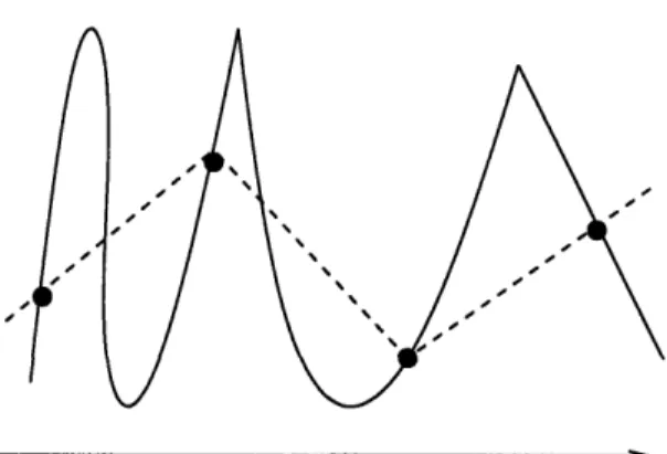
4-1 Step-up and step-down functions on the [0,1] interval ... . 75

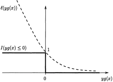
4-2 Convex loss upper-bounds the indicator loss ... 89

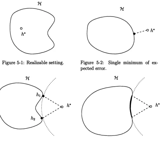
5-1 Realizable setting ... 96

5-2 Single minimum of expected error ... 96

5-3 Finite number of minimizers of expected error ... 96

5-4 Infinitely many minimizers of expected error ... 96

5-5 The most dense region of a fixed size ... 105

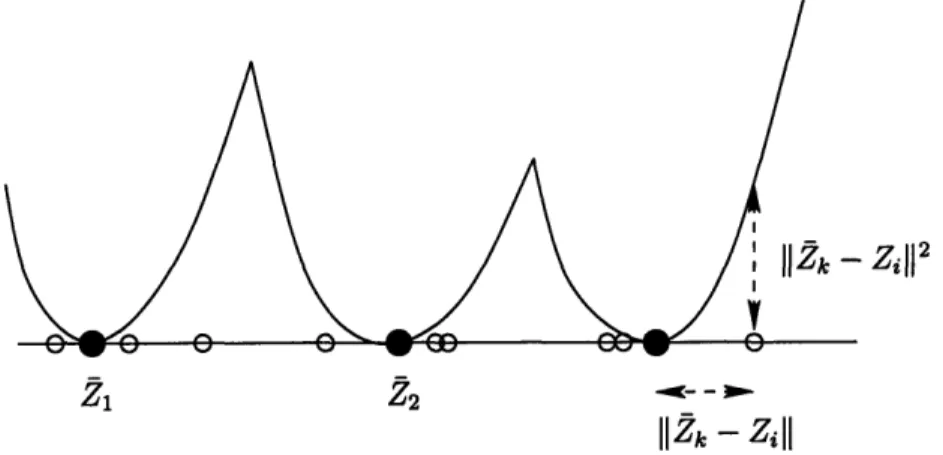
5-6 The clustering objective is to place the centers Zk to minimize the sum of squared distances from points to their closest centers ... . . 108

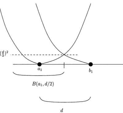
5-7 To prove Lemma 5.7.1 it is enough to show that the shaded area is upperbounded by the L1 distance between the functions hal,...,a

and

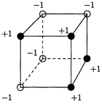
hbl,...,bK and lower-bounded by a power of d. We deduce that d cannot be large . . . 111

6-2 n-dimensional cube with a {-1, 1}-valued function defined on the ver-tices. The dashed line is the boundary separating the set of -l's from the set of l's. The points at the boundary are the "bad set" ... 123 6-3 The boundary is smallest when the cube is cut in the middle. The

extremal set is the set of points at most n/2-Hamming distance away from the origin ... 123

List of Tables

Chapter 1

Theory of Learning: Introduction

Intelligence is a very general mental capability that, among other things, involves the ability to reason, plan, solve problems, think abstractly, comprehend complex ideas,

learn quickly and learn from experience. It is not merely book learning, a narrow

academic skill, or test-taking smarts. Rather, it reflects a broader and deeper capability

for comprehending our surroundings -"catching on," "making sense" of things, or

'figuring out" what to do. [30]

The quest for building intelligent computer systems started in the 1950's, when the term "artificial intelligence" (AI) was first coined by John McCarthy. Since then, major achievements have been made, ranging from medical diagnosis systems to the Deep Blue chess playing program that beat the world champion Gary Kasparov in 1997. However, when measured against the definition above, the advances in Artificial Intelligence are still distant from their goal. It can be argued that, although the current systems can reason, plan, and solve problems in particular constrained domains, it is the "learning" part that stands out as an obstacle to overcome.

Machine learning has been an extremely active area of research in the past fifteen years. Since the pioneering work of Vapnik and Chervonenkis, theoretical foundations of learning have been laid out and numerous successful algorithms developed. This thesis aims to add to our understanding of the theory behind learning processes.

The problem of learning is often formalized within a probabilistic setting. Once such a mathematical framework is set, the following questions can be attacked:

How many examples are needed to accurately learn a concept? Will a given system be likely to give a correct answer on an unseen example? What is easier to learn and what is harder? How should one proceed in order to build a system that can learn? What are the key properties of predictive systems, and what does this knowledge tell us about biological learning?

Valuable tools and concepts for answering these questions within a probabilistic framework have been developed in Statistical Learning Theory. The beauty of the results lies in the inter-disciplinary approach to the study of learning. Indeed, a conference on machine learning would likely present ideas in the realms of Computer

Science, Statistics, Mathematics, Economics, and Neuroscience.

Learning from examples can be viewed as a high-dimensional mathematical prob-lem, and results from convex geometry and probability in Banach spaces have played an important role in the recent advances. This thesis employs tools from the theory of empirical processes to address some of the questions posed above. Without getting into technical definitions, we will now describe the learning problem and the questions studied by this thesis.

1.1 The Learning Problem

The problem of learning can be viewed as a problem of estimating some unknown

phe-nomenon from the observed data. The vague word "phephe-nomenon" serves as a common

umbrella for diverse settings of the problem. Some interesting settings considered in this thesis are classification, regression, and density estimation. The observed data is often referred to as the training data and the learning process as training.

Recall that "intelligence ... is not merely book learning." Hence, simply memo-rizing the observed data does not qualify as learning the phenomenon. Finding the right way to extrapolate or generalize from the observed data is the key problem of learning.

Let us call the precise method of learning (extrapolating from examples) an

other words, how well does the algorithm estimate the unknown phenomenon? A natural answer is to check if a new sample generated by the phenomenon fits the estimate. Finding quantitative bounds on this measure of success is one of the main problems of Statistical Learning Theory.

Since the exposition so far has been somewhat imprecise, let us now describe a few concrete learning scenarios.

One classical learning problem is recognition of hand-written digits (e.g. [24]). Such a system can be used for automatically determining the zip-code written on an envelope. The training data is given as a collection of images of hand-written digits, with the additional information, label, denoting the actual digit depicted in each image. Such a labeling is often performed by a human - a process which from the start introduces some inaccuracies. The aim is to constrict a decision rule to predict the label of a new image, one which is not in our collection. Since the new image of a hand-written digit is likely to differ from the previous ones, the system must perform clever extrapolation, ignoring some potential errors introduced in the labeling process.

Prescribing different treatments for a disease can be viewed as a complex learning problem. Assume there is a collection of therapies that could be prescribed to an ill person. The observed data consists of a number of patients' histories, with particular treatment decisions made by doctors at various stages. The number of treatments could be large, and their order might make a profound difference. Taking into account variability of responses of patients and variability of their symptoms turns this into a very complex problem. But the question is simple: what should be the best therapy strategy for a new patient? In other words, is it possible to extrapolate a new patient's treatment from what happened in the observed cases?

Spam filtering, web search, automatic camera surveillance, face recognition, finger-print recognition, stock market predictions, disease classification - this is only a small number of applications that benefited from the recent advances in machine learning. Theoretical foundations of learning provide performance guarantees for learning algo-rithms, delineate important properties of successful approaches, and offer suggestions

for improvements. In this thesis, we study two key properties of learning algorithms: their predictive ability (generalization bounds), and their robustness with respect to noise (stability). In the next two sections, we motivate the study of these properties.

1.2 Generalization Bounds

Recall that the goal of learning is to estimate the unknown phenomenon from the observed data; that is, the estimate has to be correct on unseen samples. Hence, it is natural to bound the probability of making a mistake on an unseen sample. At first, it seems magical that any such guarantee is possible. After all, we have no idea what the unseen sample looks like. Indeed, if the observed data and the new sample were generated differently, there would be little hope of extrapolating from the data. The key assumption in Statistical Learning Theory is that all the data are independently drawn from the same distribution. Hence, even though we do not know what the next sample will be, we have some idea which samples are more likely.

Once we agree upon the measure of the quality of the estimate (i.e. the error on an unseen example), the goal is to provide probabilistic bounds for it. These bounds are called performance guarantees or generalization bounds.

Following Vapnik [73], we state key topics of learning theory related to proving performance guarantees:

* the asymptotic theory of consistency of learning processes;

* the non-asymptotic theory of the rate of convergence of learning processes.

The first topic addresses the limiting performance of the procedures as the number of observed samples increases to infinity. Vaguely speaking, consistency ensures that the learning procedure estimates the unknown phenomenon perfectly with infinite

amount of data.

The second topic studies the rates of convergence (as the number of samples increases) of the procedure to the unknown phenomenon which generated the data. Results are given as confidence intervals for the performance on a given number of

samples. These confidence intervals can be viewed as sample bounds- number of examples needed to achieve a desired accuracy.

The pioneering work of Vapnik and Chervonenkis [74, 75, 76, 72], addressed the above topics for the simplest learning algorithm, Empirical Risk Minimization (ERM). Vapnik-Chervonenkis (VC) dimension, a combinatorial notion of complexity of a bi-nary function class, turned out to be the key to demonstrating uniform convergence of empirical errors to the expected performance; the result has been extended to the real-valued function classes through the notion of fat-shattering dimension by Alon et al [1]. While the theory of performance of ERM is well understood, the algorithm is impractical. It can be shown (e.g. Ben-David et al [9]) that minimizing mistakes even over a simple class of hypotheses is NP-hard. In recent years, tractable algorithms, such as Support Vector Machines [72] and Boosting [65, 27], became very popular off-the-shelf methods in machine learning. However, their performance guarantees are not as well-understood. In this thesis, we obtain generalization bounds for a family of greedy error minimization methods, which subsume regularized boosting, greedy mixture density estimation, and other algorithms.

The theory of uniform convergence, developed by Vapnik and Chervonenkis, pro-vides a bound on the generalization performance in terms of the empirical performance

for any algorithm working on a "small" function class. This generality is also a

weak-ness of this approach. In the next section, we discuss an algorithm-based approach to obtaining generalization bounds.

1.3 Algorithmic Stability

The motivation for studying stability of learning algorithms is many-fold. Let us start from the perspective of human learning. Suppose a child is trying to learn the distinction between Asian and African elephants. A successful strategy in this case is to realize that the African elephant has large ears matching the shape of Africa, while the Asian elephant has smaller ears which resemble the shape of India. After observing N pictures of each type of elephant, the child has formed some hypothesis

about what makes up the difference. Now, a new example is shown, and the child somewhat changes his mind (forms a new hypothesis). If the new example is an 'outlier' (i.e. not representative of the populations), then the child should ignore it and keep the old hypothesis. If the new example is similar to what has been seen before, the hypothesis should not change much. It can therefore be argued that a successful learning procedure should become more and more stable as the number of observations N increases. Of course, this is a very vague statement, which will be made precise in the following chapters.

Another motivation for studying stability of learning processes is to get a handle on the variability of hypotheses formed from different draws of samples. Roughly speaking, if the learning process is stable, it is easier to predict its performance than if it is unstable. Indeed, if the learning algorithm always outputs the same hypothesis, The Central Limit Theorem provides exponential bounds on the convergence of the empirical performance to the expected performance. This "dumb" learning algorithm is completely stable - the hypothesis does not depend on the observed data. Once this assumption is relaxed, obtaining bounds on the convergence of empirical errors to their expectations becomes difficult. The worst-case approach of Vapnik and Chervonenkis [74, 75] provides loose bounds for this purpose. By studying stability of the specific algorithm, tighter confidence intervals can sometimes be obtained. In fact, Rogers, Devroye, and Wagner [63, 21, 23] showed that bounds on the expected performance can be obtained for k-Nearest Neighbors and other local rules even when the VC-based approach fails completely.

If stability of a learning algorithm is a desirable property, why not try to enforce it? Based on this intuition, Breiman [17] advocated averaging classifiers to increase stability and reduce the variance. While averaging helps increase stability, its effect on the bias of the procedure is less clear. We will provide some answers to this question

in Chapter 3.

Which learning algorithms are stable? The recent work by Bousquet and Elisseeff [16] surprised the learning community by proving very strong stability of Tikhonov regularization-based methods and by deducing exponential bounds on the difference

of empirical and expected performance solely from these stability considerations. In-tuitively, the regularization term in these learning algorithms enforces stability, in agreement with the original motivation of the work of Tikhonov and Arsenin [68] on restoring well-posedness of ill-posed inverse problems.

Kutin and Nyiogi [44, 45] introduced a number of various notions of stability, showing various implications between them. Poggio et al [58, 55] made an important connection between consistency and stability of ERM. This thesis builds upon these results, proving in a systematic manner how algorithmic stability upper- and lower-bounds the performance of learning methods.

In past literature, algorithmic stability has been used as a tool for obtaining bounds on the expected performance. In this thesis, we advocate the study of stability of learning methods also for other purposes. In particular, in Chapter 6 we prove hypothesis (or L1) stability of empirical risk minimization algorithms over Donsker

function classes. This result reveals the behavior of the algorithm with respect to perturbations of the observed data, and is interesting on its own. With the help of this result, we are able to analyze sensitivity of various optimization procedures to

noise and perturbations of the training data.

1.4 Overview

Let us now outline the organization of this thesis. In Chapter 2 we introduce notation and definitions to be used throughout the thesis, as well as provide some background results. We discuss a measure of performance of learning methods and ways to esti-mate it (Section 2.2). In Section 2.3, we discuss specific algorithms, and in Sections 2.4 and 2.5 we introduce concentration inequalities and the tools from the Theory of Empirical Processes which will be used in the thesis.

In Chapter 3, we show how stability of a learning algorithm can upper- and lower-bound the bias and variance of estimators of the performance, thus obtaining perfor-mance guarantees from stability conditions.

methods. We start by proving general estimates in Section 4.1. The methods are then applied in the classification setting in Section 4.3 and in the density estimation

setting in Section 4.2.

In Chapter 5, we prove a surprising stability result on the behavior of the empirical risk minimization algorithm over Donsker function classes. This result is applied to several optimization methods in Section 5.7.

Connections are made between concentration of functions and stability in Chapter 6. In Section 6.1 we study concentration of almost-everywhere smooth functions.

1.5 Contributions

We now briefly outline the contributions of this thesis:

* A systematic approach to upper- and lower-bounding the bias and variance of estimators of the expected performance from stability conditions (Chapter 3). Most of these results have been published in Rakhlin et al [60].

* A performance guarantee for a class of greedy error minimization procedures (Chapter 4) with application to mixture density estimation (Section 4.2). Most of these results appear in Rakhlin et al [61].

* A solution to an open problem regarding L1stability of empirical risk

minimiza-tion. These results, obtained in collaboration with A. Caponnetto, are under review for publication [18].

* Applications of the stability result of Chapter 5 for optimization procedures (Section 5.7), such as finding most/least dense regions and clustering. These results are under preparation for publication.

* An extension of McDiarmid's inequality for almost-everywhere Lipschitz func-tions (Section 6.1). This result appears in Rakhlin et al [60].

* A proof of a phase transition for concentration of real-valued functions on a binary hypercube (Section 6.2). These results are in preparation for publication.

* A tight concentration of empirical errors around the mean for empirical risk minimization under a condition on the underlying space (Section 6.3). These results are in preparation for publication.

Chapter 2

Preliminaries

2.1 Notation and Definitions

The notion of a "phenomenon", discussed in the previous chapter, is defined formally as the probability space (Z, 5, P). The measurable space (Z, 5) is usually assumed to be known, while P is not. The only information available about P is through the

finite sample S = Z

1

,..., Zn} of n E Z

+

independent and identically distributed

(according to P) random variables. Note that we use upper-case letters X, Y, Z to denote random variables, while x, y, z are their realizations.

"Learning" is formally defined as finding a hypothesis h based on the observed samples Z1, . . , Zn. To evaluate the quality of h, a bounded real-valued loss (cost)

function is introduced, such that (h; z) indicates how well h explains (or fits) z. Unless specified otherwise, we assume throughout the thesis that -M <

e

< M for

some M > 0.

* Classification:

Z is defined as the product X x y, where X is an input space and y is a discrete output space denoting the labels of inputs. In the case of binary classification,

Y = {-1, 1 , corresponding to the labels of the two classes. The loss function

e

example of £ is the indicator loss:

£(yh'(x))

= I(yh'(x) < O) = I(y # sign(h'(x))).

* Regression:

Z is defined as the product X x y, where X is an input space and y is a real output space denoting the real-valued labels of inputs. The loss function £ often takes the form

£(h;

z) =

£(y-

h(x)), and the basic example is the square loss:

(y-h(x))

= (y- h(x))

2

.

* Density Estimation:

The functions h are probability densities over Z, and the loss function takes

the form

e(h;

z)

=

t(h(z)). For

instance,

t(h(z))

=

-log h(z)

is the likelihood of a point z being generated by h.

A learning algorithm is defined as the mapping

A

from samples zl, ... , z to

functions h. With this notation, the quality of extrapolation from Z, .. , Zn to a new

sample z is measured by (A(zl,.. ., zn); z).

Whenever Z = X x , it is the function h: X

-

y

that we seek. In this case,

A(Z 1,..., Zn): X y. Let us denote by

A(Z

1,..., Zn;X) the evaluation of the

function, learned on Z

1

,

.. , Z, at the point X.

Unless indicated, we will assume that the algorithm ignores the ordering of S, i.e. A(Zli,... , Zn) = A(ir(zi,...,zn)) for any permutation r E Sn, the symmetric group. If the learning algorithm

A

is clear from the context, we will write (Z1,..., Zn; )

instead of

e(A(Z

1

,..., Zn); ).

hypothe-ses available, the class

L(X)

=

{e(h;.):

h E

H}

is called the loss class.

To ascertain the overall quality of a function h, we need to evaluate the loss

e(h;.)

on an unseen sample z. Since some z's are more likely than others, we integrate over Z with respect to the measure P. Hence, the quality of h is measured by

14(h) := E(h; Z),

called the expected error or expected risk of h. For an algorithm A, its performance is the random variable

.(A(Z1,

.

Zn)) =

E [(A(Zl,.. , Zn); Z)IZ,.,

Zn].

If the algorithm is clear from the context, we will simply write

(Z

1

,...,

Zn) Since P is unknown, the expected error is impossible to compute. A major part of Statistical Learning Theory is concerned with bounding it in probability, i.e. proving

bounds of the type

((Zi,

,

Zn)

>

E)

<

(En),

where the probability is with respect to an i.i.d. draw of samples Z1

, . . .,

Zn

Such bounds are called generalization bounds or performance guarantees. In the above expression, sometimes depends on a quantity computable from the data. In the next chapter, we will consider bounds of the form

I ( 1Z(Z

1

... , Zn)- 7(Z

1

,..., Zn)

>

E)

< (e,n),

(2.1)

where t(Z

₁

,...,

Zn) is an estimate of the unknown

Z(Z

1

,...,

Zn) from the data

Z1, .. , Zn. The next section discusses such estimates (proxies) for 7R. The reader is

Table 2.1: Table of notation Z Space of samples

X, Y

Input and output spaces, whenever Z = X x y

P

Unknown distribution on Z

I,..., Zn I.i.d. sample from P n Number of samples

S

The sample {Z1,..., Zn}

e

Loss (cost) function

_____ _ Class of hypotheses

IA Learning algorithm

7. Expected error (exp. loss, exp. risk) Remp Empirical error (resubstitution estimate)

Zi1oo Leave-one-out error (deleted estimate)

lRemp Defect of the resubstitution estimate: Remp = -R lemp

R'loo Defect of the deleted estimate:

7R1oo

= R -

Rloo

conv () Convex hull of R convk (7) k-term convex hull of X

Tn(Zi,., Zn) A generic function of n random variables

un Empirical process

2.2 Estimates of the Performance

Several important estimates of the expected error R(h) can be computed from the sample. The first one is the empirical error (or resubstitution estimate),

1Remp(Zl,...

,

Zn)

:=

(Zl,...,

Zn; Zi).

i=1

The second one is the leave-one-out error (or deleted estimate)',

i n

R.1oo(Zl,, Zn) : -

e(Zl,...,

Zi-1, Zi+l,., Zn; Zi)-.

i=1

These quantities are employed to estimate the expected error, and Statistical Learning Theory is concerned with providing bounds on the deviations of these

esti-lit is understood that the first term in the sum is (Z2,... , Zn; Zi) and the last term is

Zn)-mates from the expected error. For convenience, denote these deviations

Zemp(Zli,..., Zn) i

R(Z

,.,Zn) -Zemp(Zl,...,Zn),

oo(Z1

, . .

,Zn)

:=

'(Z, .

*,Zn)

-

zioo(Z1,

***Zn). With this notation, Equation 2.1 becomes

PE

(

Zemp(Z,...,

Z.)I

>Ž

) < 6(E, n)

(2.2)

or

I

(zloo(Z,,...

,Zn)

>

6)

< (e, n)

(2.3)

If one can show that fZemp (or .10oo) is "small", then the empirical error (resp.

leave-one-out error) is a good proxy for the expected error. Hence, a small empirical (or leave-one-out error) implies a small expected error, with a certain confidence. In particular, we are often interested in the rate of the convergence of hZemp and Zlo to zero as n increases.

The goal is to derive bounds such that limn-,. 6(e, n) = 0 for any fixed > 0. If the rate of decrease of 6(e,n) is not important, we will write lRempi I 0 and

I~ool

°-O

Let us focus on the random variable Temp(Z1,... , Zn). Recall that the Central

Limit Theorem (CLT) guarantees that the average of n i.i.d. random variables con-verges to their mean (under the assumption of finiteness of second moment) quite fast. Unfortunately, the random variables

(z, .. ., Zn; ),X..., (z, .. ., Zn; Zn)

are dependent, and the CLT is not applicable. In fact, the interdependence of these random variables makes the resubstitution estimate positively biased, as the next example shows.

Example 1. Let

X

= [0, 1], Y =

{0,

1}, and

P(X) = U[O, 1], P(YIX) = jY=i.

Suppose (h(x),y) = I(h(x)

y), and A is defined as A(Zi,...,Zn;X)

=

1 if

X E X

1

,

...

, Xn} and 0 otherwise. In other words, the algorithm observes n data

points (Xi, 1), where Xi is distributed uniformly on [0, 1], and generates a hypothesis

which fits exactly the observed data, but outputs 0 for unseen points X. This situation

is depicted in Figure 2-1. The empirical error of A is 0, while the expected error is

1, i.e. fZemp(Z1,

. .. , Zn) = 1 for any Z1, .. , Z,.

1

@0

0 0

0

0-0

0

0---X1 Xn

Figure 2-1: Fitting the data.

No guarantee on smallness of 7Zemp can be made in Example 1. Intuitively, this is due to the fact that the algorithm can fit any data, i.e. the space of functions £(7i) is too large.

Assume that we have no idea what the learning algorithm is except that it picks its hypotheses from

H.

To bound lZemp, we would need to resort to the

worst-case approach of bounding the deviations between empirical and expected errors for all functions simultaneously. The ability to make such a statement is completely characterized by the "size" of £(7H), as discussed next.

2.2.1

Uniform Convergence of Means to Expectations

The class £(7) is called uniform Glivenko-Cantelli if for every e > 0,

limsupP

sup

Et-

(Z)

=

>

0,

n--boo

i

r_)

n

E

where

Zl,...,

Z are i.i.d random variables distributed according to IL.

Non-asymptotic results of the form

ED

sup

Et

-

-

E (zi) >

<

(, n,

(X))

give uniform (over the class £(7X)) rates of convergence of empirical means to expec-tations. Since the guarantee is given for all functions in the class, we immediately

obtain

PE

~ep(1

*

Zn)

>)

< (F n,

L(XH)

)

We postpone further discussion of Glivenko-Cantelli classes of functions to Section 2.5.

2.2.2 Algorithmic Stability

The uniform-convergence approach above ignores the algorithm, except for the fact that it picks its hypotheses from H. Hence, this approach might provide only loose bounds on Zemp. Indeed, suppose that the algorithm would in fact only pick one function from

X.

The bound on Zemp would then follow immediately from The Central Limit Theorem. It turns out that analogous bounds can be proved even if the algorithm picks diverse functions, as long is it is done in a "smooth" way. In Chapter 3, we will derive bounds on both Remp and lZloo in terms of various stability conditions on the algorithm. Such algorithm-dependent conditions provide guarantees for Remp and

Rloo

even when the uniform-convergence approach of Section 2.2.1 fails.

2.3 Some Algorithms

2.3.1

Empirical Risk Minimization

The simplest method of learning from observed data is the Empirical Risk

Minimiza-tion (ERM) algorithm

A(Z *,

Zn) =

ag

~mi- f(h; Z,).

h67 n

Note that the ERM algorithm is defined with respect to a class 1t. Although an exact minimizer of empirical risk in this class might not exist, an almost-minimizer always exists. This situation will be discussed in much greater detail in Chapter 5.

The algorithm in Example is an example of ERM over the function class

H=

Uh.x

=

(xl,.

. .,Xn)

E

[0, ]n}, n>1

where h,(x) = 1 if x = xi for some 1 < i < n and h:(x) = 0 otherwise.

ERM over uniform Glivenko-Cantelli classes is a consistent procedure in the sense that the expected performance converges to the best possible within the class of hypotheses.

There are a number of drawbacks of ERM: ill-posedness for general classes 7-, as well as computational intractability (e.g. for classification with the indicator loss). The following two families of algorithms, regularization algorithms and boosting

algo-rithms, aim to overcome these difficulties.

2.3.2 Regularization Algorithms

One of the drawbacks of ERM is ill-posedness of the solution. Indeed, learning can be viewed as reconstruction of the function from the observed data (inverse problem), and the information contained in the data is not sufficient for the solution to be unique. For instance, there could be an infinite number of hypotheses with zero empirical risk, as shown in Figure 2-2. Moreover, the inverse mapping tends to be

unstable.

Figure 2-2: Multiple minima of the empirical risk: two dissimilar functions fit the

data.

The regularization method described next is widely used in machine learning [57, 77], and arises from the theory of solving ill-posed problems. Discovered by J. Hadamard, ill-posed inverse problems turned out to be important in physics and statistics (see Chapter 7 of Vapnik [72]).

Let Z = X x , i.e. we consider regression or classification. The Tikhonov

regu-larization method [68], applied to the learning setting, proposes to solve the following

minimization problem

n

A(Z1

...

,

Zn)

=

argmin

(h(Xi), Y)

+

A11hIK,

i=1

where K is a positive definite kernel and 11. is the norm in the associated Reproducing Kernel Hilbert Space

i.

The parameter A > 0 controls the balance of the fit to the data (the first term) and the "smoothness" of the solution (the second term), and is usually set by a cross-validation method. It is exactly this balance between smoothness and fit to the data that restores the uniqueness of the solution. It also restores stability.

This particular minimization problem owes its success to the following surprising (although simple to prove) fact: even though the minimization is performed over a possibly infinite-dimensional Hilbert Space of functions, the solution always has the

Figure 2-3: Unique minimum of the regularized fit to the data.

form

n

A(Z

1

,.*.*,

Zn

X)

=

E3

ciK(Xi, x),

i=1

assuming that depends on h only through h(Xi).

2.3.3 Boosting Algorithms

We now describe boosting methods, which have become very popular in machine

learning [66, 27]. Consider the classification setting, i.e. Z = X x y, y =

{-1,

1}.

The idea is to iteratively build a complex classifier f by adding weighted functions

h E , where H is typically a set of simple functions. "Boosting" stands for the increase in the performance of the ensemble, as compared to the relatively weak performance of the simple classifiers. The ensemble is built in a greedy stage-wise manner, and can be viewed as an example of additive models in statistics [32].

Given a class H of "base" functions and the observed data Z1

,... ,

Z, a greedy boosting procedure builds the ensemble fk in the following way. Start with some fo = h. At the k-th step, choose ak and hk E

X

to approximately minimize the empirical error on the sample. After T steps, output the resulting classifier as

· ~~~~~

A(Z

1

,

..

.,Zn)

=

sign

(

i

hi

)

There exist a number of variations of boosting algorithms. The most popular one, AdaBoost, is an unregularized procedure with a potential to overfit if left running

for enough time. The regularization is performed as a constraint on the norm of the coefficients or via early stopping. The precise details of a boosting procedure with the constraint on the

E

1 norm of the coefficients are given in Chapter 4, where a bound

on the generalization performance is proved.

2.4 Concentration Inequalities

In the context of learning theory, concentration inequalities serve as tools for obtain-ing generalization bounds. While deviation inequalities are probabilistic statements about the deviation of a random variable from its expectation, the term "concentra-tion" often refers to the exponential bounds on the deviation of a function of many random variables from its mean. The reader is referred to the excellent book of Ledoux [47] for more information on the concentration of measure phenomenon. The well-known probabilistic statements mentioned below can be found, for instance, in the survey by Boucheron et al [13].

Let us start with some basic probability inequalities. For a non-negative random

variable X,

EX= j

(X > t)dt.

The integral above can be lower-bounded by the product t (X

>

t) for any fixed t > 0. Hence, we obtain Markov's inequality:

EX

P(X> t)

t

for a non-negative random variable X and any t > 0.

For a non-negative strictly monotonically increasing function q,

P (X > t) = P (0(X) > 0(t)),

resulting in

EO(x

)

P(X > t) <qE()

for an arbitrary random variable X.

Setting 0(x) = Xq for any q > 0 leads to the method of moments

(IX- EXI > t) < EJX -EXIq

for any random variable X. Since the inequality holds for any q > 0, one can optimize the bound to get the smallest one. This idea will be used in Chapter 6. Setting q = 2 we obtain Chebyshev's inequality which uses the second-moment information to bound the deviation of X from its expectation:

VarX

(IX- EXl > t) <

V

.

Other choices of b lead to useful probability inequalities. For instance, O(x) = e x

for s > 0 leads to the Chernoff's bounding method. Since

P (X > t)

= P (esx

>

eat)

we obtain

P

(X > t) <

Eex

eat

Once some information about X is available, one can minimize the above bound over

s >0.

So far, we have discussed generic probability inequalities which do not exploit any "structure" of X. Suppose X is in fact a function of n random variables. Instead of

the letter X, let us denote the function of n random variables by T.(Z,

. . .,

Z).

Theorem 2.4.1 (Hoeffding [34]). Suppose T,(Z, Z* * = = l Zi, where Zi 's are

independent and ai < Zi

bi. Then for any e > 0,

-2C2

P (ITn- ETn I > e) < 2e r?=i(bi-ai)

Hoeffding's inequality does not use any information about the variances of Zi's. A tighter bound can be obtained whenever these variances are small.

Theorem 2.4.2 (Bennett [10]). Suppose T(Z

1

,..., Zn)

=

Einl

Zi, where Zi's are

independent, and for any i, EZi = 0 and

IZi

< M. Let

2 =

I

Z

Var{Z}. Then

for any

£

>

0,

no2

IP(ITnI

> e)

<

2exp -- f

(

EM

where 4(x) = (1 + x) log(1 + x) - x.

Somewhat surprisingly, exponential deviation inequalities hold not only for sums, but for general "smooth" functions of n variables.

Theorem 2.4.3 (McDiarmid [54]). Let T : Z

n

_{- R such that}

Vz1, ,Zn, Z1 ... Zn E Tn(zl,. ,Zn) - Tn(Zl,. ,Zi, , n) < Ci

Let Z1, . . ., Z be independent random variables. Then

) > ) < exp (

<-E)

< exp (

n 2 c

2 i=l 'i

The following Efron-Stein's inequality can be used to directly upper-bound the variance of functions of n random variables.

Theorem 2.4.4 (Efron-Stein [26]). Let

Tn

: Z

'-* R be a measurable function of n

n

variables and define F = Tn(Z

1

, .

. Zn)

and

F'

Tn(Z,

. . . Z,

Z

I

,

..

,

Zn),

where

Z,a,

. r nm

Zvr

b e

Zn

are i.i.d. random variables. Then

n

Var(Tn) < E E

i=1

A "removal" version of the above is the following:

(2.4)

and

E2

En 1 C?,

Theorem 2.4.5 (Efron-Stein). Let Tn : Z - R be a measurable function of n

variables and T : Z-

- R of n - 1 variables. Define

r

= Tn(Z

1

, ..

, Zn) and

ri

= T(Z,...,

Zi-

1

, Zi+,..., Zn),

where

Z

1

,..., Zn

are i.i.d. random variables. Then

n

Var(Tn) <

E

[(r

- )2] (2.5)

i=1

A collection of random functions Tn for n = 1, 2, ... can be viewed as a sequence of random variables

{Tn}.

There are several important notions of convergence of sequences of random variables: in probability and almost surely.

Definition 2.4.1. A sequence {Tn}, n = 1,2,..., of random variables converges to

T in probability

Tn __ T

if for each > 0

lim P (ITn - T

>

) = 0.

n--oo

This can also be written as

P?

(IT - T > e) -- 0.

Definition 2.4.2. A sequence

{Tn},

n = 1,2,..., of random variables converges to

T almost surely if

1P

( lim Tn

=

T)

=

O.

Deviation inequalities provide specific upper bounds on the convergence of

P(IT --TI > )

-+0.

Assume for simplicity that Tn is a non-negative function and the limit T is 0. When inspecting inequalities of the type

it is often helpful to keep in mind the two-dimensional surface depicted in Figure 2-4. For a fixed n, decreasing increases P (Tn

>

e). For a fixed , P

(T, > e)

-- 0 as

n -

oc.

Now, suppose that we would like

e

to decrease with n. One can often find the fastest possible decay e(n), such that P (Tn

>

e(n)) -- 0 as n oo. This defines the rate of convergence of Tn to 0 in probability. In Chapter 5 we study rates of decay of certain quantities in great detail.

6

Figure 2-4: Probability surface

Let us conclude this Section by reminding the reader about the order notation. Let f(n) and g(n) be two functions.

Definition 2.4.3 (Asymptotic upper bound).

f(n)

E

O(g(n)) if lim

f')

<

X.

Definition 2.4.4 (Asymptotically negligible).

g(n)

Definition 2.4.4 (Asymptotically negligible).

f(n)

E

o(g(n))

if

lim f

_)=o.

Definition 2.4.5 (Asymptotic lower bound).

f(n) E (g(n)) if lim f(n) > 0.

n-too g(n)

In the above definitions, "" will often be replaced by "=".

2.5 Empirical Process Theory

In this section, we briefly mention a few results from the Theory of Empirical Pro-cesses, relevant to this thesis. The reader is referred to the excellent book by A. W. van der Waart and J. A. Wellner [71].

2.5.1

Covering and Packing Numbers

Fix a distance function d(f, g) for f, g E

X.

Definition 2.5.1. Given > 0 and hl,...

,hN

E -, we say that hl,...,hN

are

e-separated if d(hi, hj) > e for any i

#

j.

The e-packing number, D(7-, E, d), is the maximal cardinality of an e-separated

set.

Definition 2.5.2. Given e > 0 and h1,..., hN E

7',

we say that the set h1, ... , hN

is an e-cover of 7-I if for any h E 7', there exists 1 < i < N such that d(h, hi) < e. The e-covering number, A(-, e, d), is the minimal cardinality of an e-cover of X. Furthermore, log Af(H, e, d) is called metric entropy.

It can be shown that

D(-, 2E, d) < (7, ,d)

<

D(V(,E, d).

Definition 2.5.3. Entropy with bracketing

ArN

(7-, e, d) is defined as the smallest

num-ber N for which there exists pairs {hi, h}S_

1

such that d(hi, hi) < E for all i and for

2.5.2

Donsker and Glivenko-Cantelli Classes

Let

P,

stand for the discrete measure supported on Z1, .. ,

Z,.

More precisely,

n=

zziX

the sum of Dirac measures at the samples. Throughout this thesis, we will denote

n

Pf

=

Ezf (Z)

and

Pnf

=

f(Zi)

i=1

Define the sup norm as

IIQf

II,

= sup IQf

I

feY

for any measure

Q.

We now introduce the notion of empirical process.

Definition 2.5.4. The empirical process

vn,

indexed by a function class F is defined as the map

n

f

n(f) =

-(Pn

-

P)f

=

E(f(zi)

-

Pf

v\/ni=1

The Law of Large Numbers (LLN) guarantees that Pnf converges to Pf for a fixed

f,

if the latter exists. Moreover, the Central Limit Theorem (CLT) guaran-tees that the empirical process

vn(f)

converges to N(O, P(f - Pf) 2) if pf 2

is

finite. Similar statements can be made for a finite number of functions simultaneously. The analogous statements that hold uniformly over infinite function classes are the core topic of Empirical Process Theory.

Definition 2.5.5. A class

F'

is called P-Glivenko-Cantelli if

ijPn - PIL P* 0,

Definition 2.5.6. A class

F

is called P-Donsker if

LEn V

in

£oo(),

where the limit

v

is a tight Borel measurable element in £'(F) and "a"

denotes weak convergence, as defined on p. 17 of [71].

In fact, it follows that the limit process must be a zero-mean Gaussian process with covariance function Ev (f)v(f') = (f, f') (i.e. a Brownian bridge).

While Glivenko-Cantelli classes of functions have been used in Learning Theory to a great extent, the important properties of Donsker classes have not been utilized. In Chapter 5, P-Donsker classes of functions play an important role because of a specific covariance structure they possess. We hypothesize that many more results can be discovered for learning with Donsker classes.

Various Donsker theorems provide sufficient conditions for a class being P-Donsker. Here we mention a few known results (see [71], Eqn. 2.1.7 and [70], Thin. 6.3) in terms of entropy logAf and entropy with bracketing log./'N.

Proposition 2.5.1. If the envelope F of F is square integrable and

j

sup logJ\(e

IIFIIQ

, F, L₂(Q))de < o,

then F is P-Donsker for every P, i.e.

is a universal Donsker class. Here the

supremum is taken over all finitely discrete probability measures.

Proposition 2.5.2. If

f0

/log0Af

(e, ,

L

2

(P))de < oo, then F

is P-Donsker.

From the learning theory perspective, however, the most interesting theorems are probably those relating the Donsker property to the VC-dimension. For example, if F

is a {0, 1}-valued class, then F is universal Donsker if and only if its VC dimension is finite (Thin. 10.1.4 of [25] provides a more general result involving Pollard's entropy condition). As a corollary of their Proposition 3.1, [29] show that under the Pollard's entropy condition, the 0, 1}-valued class F is in fact uniform Donsker. Finally,

Rudelson and Vershynin [64] extended these results to the real-valued case: a class F is uniform Donsker if the square root of its VC dimension is integrable.

2.5.3 Symmetrization and Concentration

The celebrated result of Talagrand [67] states that the supremum of an empirical process is tightly concentrated around its mean. The version stated below is taken from [6].

Theorem 2.5.1 (Talagrand). Let F be a class of functions such that

IlfII,

< b

for every f E

F.

Suppose, for simplicity, that Pf = 0 for all f E

F.

Let a2 =

V/isupfE:FVar(f). Then, for every e >

0,

P

(I[vnI

lED(§I~nilF-tllonlsl>E)CeX~Kb

-

Ellv.I]l

I>

E)

<

C exp

-

-

log

1+

0og

+

2+ 21

bEll

bE

V.11 ))

)

where C and K are absolute constants.

The above Theorem is key to obtaining fast rates of convergence for empirical risk minimization. The reader is referred to Bartlett and Mendelson [6].

It can be shown that the empirical process

1 n

f

-4

vn(f)

=

(Pn-P)f

=

/i

(f(Z)

-

Pf)

is very closely related to the symmetrized (Rademacher) process

1

n

f

7n

(f)

=

fI

eif(Zi),

i=1

where el, .E. , n are i.i.d. Rademacher random variables, independent of

Zl, . ..,

Z,

such that P (i = -1) = P (i = +1) = 1/2. In fact, the LLN or the CLT for one process holds if and only if it holds for the other [71].

Since we are interested in statements which are uniform over a function class, the object of study becomes the supremum of the empirical process and the supremum of

the Rademacher process. The Symmetrization technique [28] is key to relating these two.

Lemma 2.5.1 ([71] Symmetrization). Consider the following suprema:

i n 1

Zn(X,..., Xn) = sup Ef-Z

E

f(Xi)

=

111n11y

and

Rn(Xi,

**X)

=

sup

ef(X)

|=1

nIF

fEY n.f*(X

?nII

Then

EZn < 2ERn.

The quantity ERP is called the Rademacher average of .F.

Consider functions with bounded Lipschitz constant. It turns out that such func-tions can be "erased" from the Rademacher sum, as stated in Lemma 2.5.2.

Definition 2.5.7. A function : R - R is a contraction if

q(0) = 0 and

10(s) - OWt < s - t .

We will denote fi = f(xi). The following inequality can be found in [46], Theorem 4.12.

Lemma 2.5.2 ([46] Comparison inequality for Rademacher processes). If

qi:

R R

(i = 1, .., n) are contractions, then

n n

EEsup Zeioi(fi) < 2EEsup

Zeifi

fE6 i-1 fEi- 1

In Chapter 4, this lemma will allow us to greatly simplify Rademacher complexities over convex combinations of functions by "erasing" the loss function.

Chapter 3

Generalization Bounds via

Stability

The results of this Chapter appear in [60].

3.1 Introduction

Albeit interesting from the theoretical point of view, the uniform bounds, discussed in Section 2.2.1, are, in general, loose, as they are worst-case over all functions in the class. As an extreme example, consider the algorithm that always ouputs the same function (the constant algorithm)

A(Z,

.,

Zn)

= fo, V(Zi,,

Z.)

E Z

.

The bound on Temp(Z,.. , Zn) follows from the CLT and an analysis based upon

the complexity of a class 7T does not make sense.

Recall from the previous Chapter that we would like, for a given algorithm, to obtain the following generalization bounds

with

6(e,

n) -- 0 as n oo.

Throughout this Chapter, we assume that the loss function

e

is bounded and non-negative, i.e.

0 <

e

< M. Notice that Remp and

ZIoo

are bounded random variables.

By Markov's inequality,

V'E

> 0,

P

(Ifempl _ E) EI7mpl

and also

*1'

> 0,

EIlZempl

<

MP

(Ifempl > e ) + '.

Therefore, showing Rzemp L 0 is equivalent to showing EIlempl- O.

The latter is equivalent to

E(Zemp) 2 + 0 since IlZempl < M. Further notice that

E(lZemp) = Var(emp) + (EZemp)

2

We will call ErZemp the bias, Var(Zemp) the variance, and E(Zemp)2 the second

mo-ment of emp. The same derivations and terminology hold for

7f1Zo.

Hence, studying conditions for convergence in probability of the estimators to zero is equivalent to studying their mean and variance (or the second moment alone).

In this Chapter we consider various stability conditions which allow one to bound bias and variance or the second moment, and thus imply convergence

of

Rfemp and 1Zoo to zero in probability. Though the reader should expect a number of definitions of stability, the common flavor of these notions is the comparison of the "behavior" of the algorithm A on similar samples. We hope that the present work sheds light on the important stability aspects of algorithms, suggesting principles for designing