HAL Id: hal-00639522
https://hal.archives-ouvertes.fr/hal-00639522
Submitted on 9 Nov 2011
HAL is a multi-disciplinary open access
archive for the deposit and dissemination of
sci-entific research documents, whether they are
pub-lished or not. The documents may come from
teaching and research institutions in France or
abroad, or from public or private research centers.
L’archive ouverte pluridisciplinaire HAL, est
destinée au dépôt et à la diffusion de documents
scientifiques de niveau recherche, publiés ou non,
émanant des établissements d’enseignement et de
recherche français ou étrangers, des laboratoires
publics ou privés.
Local Optima Networks with Escape Edges
Sébastien Verel, Fabio Daolio, Gabriela Ochoa, Marco Tomassini
To cite this version:
Sébastien Verel, Fabio Daolio, Gabriela Ochoa, Marco Tomassini. Local Optima Networks with Escape
Edges. International Conference on Artificial Evolution (EA-2011), Oct 2011, Angers, France. pp.10
- 23. �hal-00639522�
Local Optima Networks with Escape Edges
Sebastien Verel
2
, Fabio Daolio
3
, Gabriela Ochoa
1
, Marco Tomassini
3
1
School of Computer Science, University of Nottingham, Nottingham, UK.
2
INRIA Lille - Nord Europe and University of Nice Sophia-Antipolis, France.
3
Faculty of Business and Economics, University of Lausanne, Lausanne, Switzerland.
Abstract. This paper proposes an alternative definition of edges (escape edges)
for the recently introduced network-based model of combinatorial landscapes:
Local Optima Networks (LON). The model compresses the information given by
the whole search space into a smaller mathematical object that is the graph
hav-ing as vertices the local optima and as edges the possible weighted transitions
between them. The original definition of edges accounted for the notion of
tran-sitions between the basins of attraction of local optima. This definition, although
informative, produced densely connected networks and required the exhaustive
sampling of the basins of attraction. The alternative escape edges proposed here
do not require a full computation of the basins. Instead, they account for the
chances of escaping a local optima after a controlled mutation (e.g. 1 or 2
bit-flips) followed by hill-climbing. A statistical analysis comparing the two LON
models for a set of N K landscapes, is presented and discussed. Moreover, a
pre-liminary study is presented, which aims at validating the LON models as a tool for
analyzing the dynamics of stochastic local search in combinatorial optimization.
1
Introduction
The performance of heuristic search algorithms crucially depends on the structural
as-pects of the spaces being searched. An improved understanding of this dependency,
can facilitate the design and further successful application of these methods to solve
hard computational search problems. Local optima networks (LON) have been recently
introduced as a novel model of combinatorial landscapes [10, 11]. This model allows
the use of complex network analysis techniques [7] in connection with the study of
fitness landscapes and problem difficulty in combinatorial optimization. The model is
based on the idea of compressing the information given by the whole problem
config-uration space into a smaller mathematical object, which is the graph having as vertices
the optima configurations of the problem and as edges the possible transitions between
these optima. This characterization of landscapes as networks has brought new insights
into the global structure of the landscapes studied, particularly into the distribution of
their local optima. Moreover, some network features have been found to correlate and
suggest explanations for search difficulty on the studied domains.
The definition of the edges in the LON model critically impacts upon its
descrip-tive power with regards to heuristic search. The initial definition of edges in [10, 11],
basin-transition
edges, accounted for the notion of transitions between the local optima
basins’ frontiers. This definition, although informative, produces highly connected
net-works and requires the exhaustive sampling of the basins of attraction. We explore in
II
S. Verel, F. Daolio, G. Ochoa, and M. Tomassini
this article an alternative definition of edges, which we term escape edges, that does not
require a full computation of the basins. Instead, the edges account for the chances (of
a prospective heuristic search algorithm) of escaping a local optima after a controlled
mutation (e.g. 1 or 2 bit-flips) followed by hill-climbing. This new definition produces
less dense and easier to build LONs, which are more amenable to sampling and get
us closer to a fitness landscape model that can be used to understand (and eventually
exploit) the dynamics of local search on combinatorial problems.
The first goal of the present study is to compare and explore the relationships
be-tween the two LON models, based on (i) basin-transition edges and (ii) escape edges,
respectively. Thereafter, we present a preliminary study that aims at validating the LON
models in their descriptive power of the dynamics of stochastic local search algorithms.
We conduct this validation by considering the behavior of two well-known stochastic
local search heuristics, namely, Tabu Search [4] and Iterated Local Search [6]. The well
known family of N K landscapes [5] is used in our study.
The article is structured as follows. Section 2, includes the relevant definitions and
algorithms for extracting the LONs. Section 3, describes the experimental design, and
reports a comparative analysis of the extracted networks of the two models. Section 4,
presents our model validation study. Finally, section 5 discusses our main findings and
suggest directions for future work.
2
Definitions and algorithms
A Fitness landscape [9] is a triplet (S, V, f ) where S is a set of potential solutions i.e.
a search space, V : S −→ 2
S
, a neighborhood structure, is a function that assigns to
every s ∈ S a set of neighbors V (s), and f : S −→ R is a fitness function that can be
pictured as the height of the corresponding solutions. In our study, the search space is
composed of binary strings of length N , therefore its size is 2
N
. The neighborhood is
defined by the minimum possible move on a binary search space, that is the single
bit-flip operation. Thus, for a bit string s of length N , the neighborhood size is |V (s)| = N .
The HillClimbing algorithm to determine the local optima and therefore define the
basins of attraction, is given in Algorithm 1. It defines a mapping from the search space
S to the set of locally optimal solutions S
∗
. Hill climbing algorithms differ in their
so-called pivot-rule. In best-improvement local search, the entire neighborhood is explored
and the best solution is returned, whereas in first-improvement, a neighbor is selected
uniformly at random and is accepted if it improves on the current fitness value. We
consider here a best-improvement local searcher (see Algorithm 1). For a comparison
between first and best-improvement LON models, the reader is referred to [8]
2.1
Nodes
As discussed above, a best-improvement local search algorithm based on the 1-move
operation is used to determine the local optima. A local optimum (LO), which is taken
to be a maximum here, is a solution s
∗
such that ∀s ∈ V (s), f (s) ≤ f (s
∗
).
Let us denote by h(s), the stochastic operator that associates to each solution s,
the solution obtained after applying the best-improvement hill-climbing algorithm (see
Local Optima Networks with Escape Edges
III
Algorithm 1 Best-improvement local search (hill-climbing).
Choose initial solution s ∈ S
repeat
choose s
0
∈ V (s), such that f (s
0
) = max
x∈V (s)
f (x)
if f (s) < f (s
0
) then
s ← s
0
end if
until s is a Local optimum
Algorithm 1) until convergence to a LO. The size of the landscape is finite, so we can
denote by LO1, LO2, LO3
. . . , LOp, the local optima. These LOs are the vertices of
the local optima network.
2.2
Basin-transition edges
The basin of attraction of a local optimum LOi
∈ S is the set bi
= {s ∈ S | h(s) =
LOi}. The size of the basin of attraction of a local optimum i is the cardinality of bi,
denoted ]bi. Notice that for non-neutral
4
fitness landscapes, as are standard N K
land-scapes, the basins of attraction as defined above, produce a partition of the configuration
space S. Therefore, S = ∪i∈S
∗
b
i
and ∀i ∈ S ∀j 6= i, bi
∩ b
j
= ∅.
We can now define the weight of an edge that connects two feasible solutions in the
fitness landscape. For each pair of solutions s and s
0
, p(s → s
0
) is the probability to pass
from s to s
0
with the given neighborhood structure. In the case of binary strings of size
N , and the neighborhood defined by the single bit-flip operation, there are N neighbors
for each solution, therefore, considering a uniform selection of random moves:
if s
0
∈ V (s) , p(s → s
0
) =
N
1
and
if s
0
6∈ V (s) , p(s → s
0
) = 0.
The probability to go from solution s ∈ S to a solution belonging to the basin bj
, is
5
:
p(s → bj
) =
X
s
0
∈b
j
p(s → s
0
)
.
Thus, the total probability of going from basin bi
to basin bj
, i.e. the weight wij
of edge
e
ij
, is the average over all s ∈ b
i
of the transition probabilities to solutions s
0
∈ b
j
:
p(b
i
→ b
j
) =
1
]bi
X
s∈b
i
p(s → b
j
)
.
2.3
Escape edges
The escape edges are defined according to a distance function d (minimal number of
moves between two solutions), and a positive integer D > 0.
4
For a definition of basins that deals with neutrality, the reader is referred to [11].
5
Notice that p(s → b
j
) ≤ 1 and notice also that this definition, disregarding the fitness values,
IV
S. Verel, F. Daolio, G. Ochoa, and M. Tomassini
There exists an edge eij
between LOi
and LOj
if it exists a solution s such that
d(s, LOi) ≤ D and h(s) = LOj. The weight wij
of this edge is then: wij
= ]{s ∈
S | d(s, LOi) ≤ D and h(s) = LOj}, which can be normalized by the number of
solutions within reach w.r.t. such a distance ]{s ∈ S | d(s, LOi) ≤ D}.
2.4
Local optima network
The weighted local optima network Gw
= (N, E) is the graph where the nodes ni
∈ N
are the local optima, and there is an edge eij
∈ E, with weight wij
= p(b
i
→ bj),
between two nodes ni
and nj
if p(bi
→ bj) > 0.
According to both definitions of edge weights, wij
= p(b
i
→ b
j) may be different
than w
ji
= p(b
j
→ b
i). Thus, two weights are needed in general, and we have an
oriented transition graph.
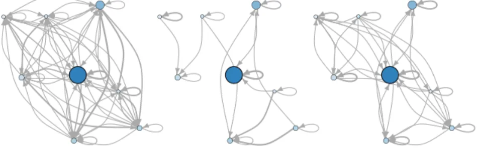
Figure 1 depicts a representative example of the alternative LON models. The
fig-ures corresponds to a real N K landscape with N = 18, K = 2, which is the lowest
ruggedness value explored in our study. The left plot illustrates the basin-transition
edges, while the center and right plots the escape edges with D = 1 and D = 2,
respectively. Notice that the basin-transition edges (left) produce a densely connected
network, while the escape edges produce more sparse networks.
●
●
●
●
● ●●
●
●
●
●
● ●●
●
●
●
●
● ●●
Fig. 1. Local optima network of an N K-landscape instance with N = 18, K = 2. Left:
basin-transition edges. Center and Right: escape edges with D = 1 and D = 2, respectively. The
size of the circles is proportional to the logarithm of the size of the corresponding basins of
attraction; the darker the color, the better the local optimum fitness. The edges’ width scales with
the transition probability (weight) between local optima, according to the respective definitions.
Notice that the basin-transition edges model (Left) is much more densely connected.
3
Comparative analysis of the LON models
In this section, we compare the LONs resulting from the different edges definitions
discussed above. We chose to perform this analysis on the N K-model artificial
land-scapes, primarily to be able to compare directly with previous work [10, 11], but also
Local Optima Networks with Escape Edges
V
because this problem provides a framework that is of general interest in studying the
structure of complex combinatorial problems [5].
The N K family of correlated landscapes is in fact a problem-independent model for
constructing multimodal landscapes that can gradually be tuned from smooth to rugged.
In the model, N refers to the number of (binary) genes in the genotype, i.e. the string
length, and K to the epistatic interaction, i.e. the number of genes that influence a
par-ticular gene. By increasing the value of K from 0 to N − 1, the landscapes can be tuned
from smooth to rugged. The K variables that form the context of the fitness
contribu-tion of a gene, can be chosen according to different models, the two most widely studied
being the random neighborhood model and the adjacent neighborhood model. As no
significant differences between the two were found, neither in terms of the landscape
global properties [5] nor in terms of their local optima networks (preliminary studies),
we conduct our full study on the more general random model.
In order to minimize the influence of the random creation of landscapes, we
consid-ered 30 different and independent problem instances for each combination of N and K
parameter values. In all cases, the measures reported are the average of these 30
land-scapes. In the present study, N = 18 and K ∈ {2, 4, 6, 8, 10, 12, 14, 16, 17}, which
are the largest possible parameter combinations that allow the exhaustive extraction of
local optima networks. LONs for the two definitions of edges: (i) basin-transition and
(ii) escape edges with D ∈ {1, 2}, were extracted and analyzed
6
.
Table 1. Local optima network features. Values are averages over 30 random instances, standard
deviations are shown as subscripts. K = epistasis value of the corresponding N K-landscape
(N = 18); N
v
= number of vertices; D
edge
= density of edges (N
e
/(N
v
)
2
× 100%); L
opt
=
average shortest path to reach the global optimum (d
ij
= 1/w
ij
).
K
N
v
D
edge
(%)
L
opt
all
Basin-trans.
Esc.D1
Esc.D2
Basin-trans. Esc.D1 Esc.D2
2
43.0
27.7
74.182
13.128
8.298
4.716
22.750
9.301
21.2
8.0
16.8
4.7
33.5
14.1
4
220.6
39.1
54.061
4.413
1.463
0.231
7.066
0.810
41.7
10.5
19.2
5.1
53.7
12.4
6
748.4
70.2
26.343
1.963
0.469
0.047
3.466
0.279
80.0
19.1
22.2
3.9
66.7
12.9
8
1668.8
73.5
12.709
0.512
0.228
0.009
2.201
0.066
110.1
13.8
24.0
4.9
76.6
9.1
10 3147.6
109.9
6.269
0.244
0.132
0.004
1.531
0.036
152.8
19.3
27.3
5.0
90.7
8.4
12 5270.3
103.9
3.240
0.079
0.088
0.001
1.115
0.015
185.1
23.8
30.3
6.7
108.3
12.3
14 8099.6
121.1
1.774
0.035
0.064
0.001
0.838
0.009
200.2
16.0
38.9
9.6
124.7
8.6
16 11688.1
101.3
1.030
0.013
0.051
0.000
0.647
0.004
211.8
15.0
47.9
11.4
146.2
11.2
17 13801.0
74.1
0.801
0.007
0.047
0.000
0.574
0.002
214.3
17.5
55.7
12.5
155.9
12.2
3.1
Network features and connectivity
Number of nodes and edges. The 2
nd
column of Table 1, reports the number of nodes
(local optima), Nv, which is the same for all the studied landscapes and models. The
6
Some of the the tools for fitness landscape analysis and the local search heuristics, were used
from the “ParadisEO” library [2]; data treatment and network analysis are done in “R” with
the “igraph” package [3].
VI
S. Verel, F. Daolio, G. Ochoa, and M. Tomassini
number of nodes increase exponentially with increasing values of K. The networks,
however, have a different number of edges, as can be appreciated in the 3
rd
, 4
th
, and
5
th
columns of Table 1, which report the number of edges normalized by the square
of the number of nodes (density of edges). Clearly, the density is higher for the
basin-transition edges, followed by the escape edges with D = 2, and the smaller density
corresponds to D = 1. The trend is, however, that density decreases steadily with
increasing values of K, which supports the correlation between the two models.
With the basin-transition edges, LONs are densely connected, especially when K
is low: 74% and 54% of all possible edges are present, on average, for K ∈ {2, 4}.
The escape edges produce sparsely connected graphs. Indeed, the D = 1-escape edge
model, produces networks that are not completely connected, with the number of
con-nected components ranging between 1.67 and 8.37 in average. The global optimum,
though, always happens to belong to the largest connected component, which, in our
analysis, comprises an average proportion of solutions raising, with increasing values
of K, from 0.9392764 to 0.9999879.
The networks with escape edges and D = 2, are always connected. The density
decreases with the epistasis degree. For high Ks, the density values are close to those
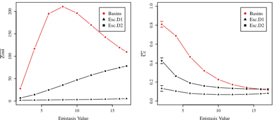
of the basin-transition networks. Figure 2 (Left) illustrates what is happening in terms
of the average degree of the outgoing links. First, notice that the difference with the
basin-transition networks is maximal when K is between 4 and 12. Whereas for D = 1
the outgoing degree only increases from 1.7 to 5.5 across the range of K values, for
D = 2 the growth is faster and reaches 78.2, not far from the 109.5 score of the LON
with basin-transition edges. The size of the basins could provide an explanation for this:
at high values of K basins are so small that a 2-bit mutation from the local optimum is
almost enough to recover the complete topology.
● ● ● ● ● ● ● ● ●
5
10
15
0
50
100
150
200
Epistasis Value
Z
o
u
t
● ● ● ● ● ● ● ● ●●
Basins
Esc.D1
Esc.D2
● ● ● ● ● ● ● ● ●5
10
15
0.0
0.2
0.4
0.6
0.8
1.0
Epistasis Value
C
c
● ● ● ● ● ● ● ● ●●
Basins
Esc.D1
Esc.D2
Fig. 2. Average out-degree (Left) and average clustering coefficient (Right) vs epistasis value.
Clustering coefficient. LONs with basins-transitions edges present a somewhat
symmetric structure: when two nodes i and j are connected, both edges eij
and eji
are present (even though their weights are in general different, wij
6= wji). Moreover,
Local Optima Networks with Escape Edges
VII
those connections often form triangular closures whose frequency is given by the global
clustering coefficient. As Figure 2 (Right) shows, this measure of transitivity is lower
with the escape-transition edges, but the difference could be due to the different number
of edges of those LONs. Values for D = 1 are remarkably low, even if the calculation
disregarded the direction of edges. Overall though, the decreasing trend w.r.t. the
land-scape ruggedness, remains common. In other words, even with eland-scape-transition edges,
the clustering coefficient can be retained as a measure related to problem complexity: it
decreases with the non-linearity of the (N K-) problem.
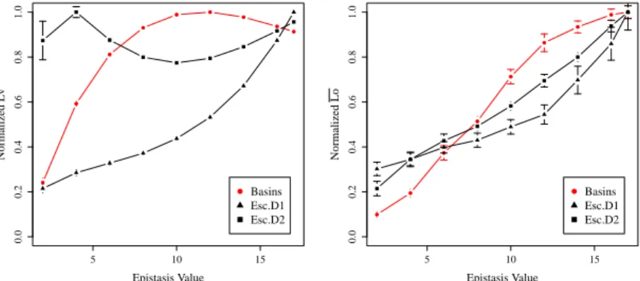
Shortest paths. Due to the differences in topology, in the escape edges networks
not all the paths are possible: few nodes might be disconnected, or they might not be
reachable due to direction constraints (these are more “asymmetric” networks, as can be
seen in Fig. 1). Thus, while evaluating shortest paths, only paths connecting reachable
couples of nodes are averaged. Moreover, there are different ranges of weights, so the
values displayed in Figure 3 have been normalized. An unexpected behavior can be
observed for D = 2: the average path length peaks at K = 4 and stays always high.
Maybe the increasing connectivity of nodes (see Fig. 2) counteracts their increase in
numbers. However, some paths are more important than others, for example those who
lead to the global optimum (see Fig. 3 (right)). With respect to these paths, all the LON
models show the same trend: the paths increase in length as ruggedness increases.
● ● ● ● ● ● ● ● ●
5
10
15
0.0
0.2
0.4
0.6
0.8
1.0
Epistasis Value
Normalized
L
v
● ● ● ● ● ● ● ● ●●
Basins
Esc.D1
Esc.D2
● ● ● ● ● ● ● ● ●5
10
15
0.0
0.2
0.4
0.6
0.8
1.0
Epistasis Value
Normalized
L
o
● ● ● ● ● ● ● ● ●●
Basins
Esc.D1
Esc.D2
Fig. 3. Shortest paths over the LON vs epistasis value. Left: average geodesic distance between
optima. Right: average shortest path to the global optimum. Each curve has been divided by its
respective maximum value.
3.2
Characterization of weights
Disparity. Figure 2 (Left) gave the average connectivity of vertices, counting outgoing
links. One might then ask whether or not there are preferential directions when leaving
a particular basin, i.e. if for a given node i, the weights wij
(with j 6= i) are equivalent.
For this purpose, we measure the disparity Y2
[1], which gauges the heterogeneity of
the contributions of the edges of node i to the total weight. For a large enough degree
VIII
S. Verel, F. Daolio, G. Ochoa, and M. Tomassini
zi, when there is not a dominant weight, then Y2
≈ 1/zi. The connectivity of LONs
with escape edges with D = 1 is weak, and it is difficult to draw conclusions based on
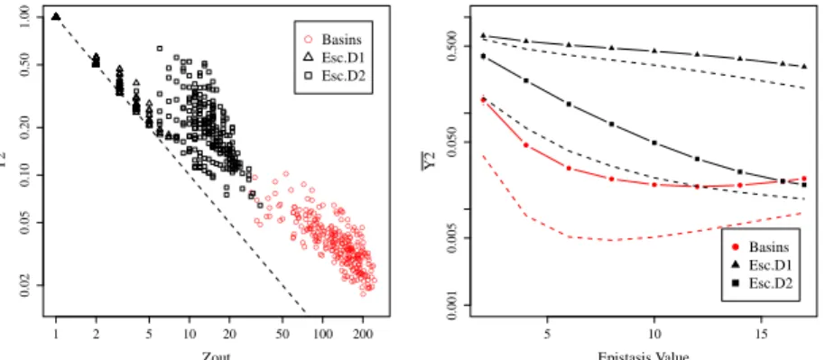
disparity only, as Figure 4 (left) illustrates. In the example illustrated, where K = 4,
(i.e. relatively low epistasis, and so not a random structure), Y2
approaches 1/z for
escape-D = 1, whereas it has distinctively higher values for both the escape-D = 2,
and the basin-transition edges.
However, the common trend is that disparity decreases with increasing epistasis: as
the landscapes become more rugged, the transition probabilities to leave a particular
basins appear to become more uniform, which could relate to the search difficulty. This
is clear from Fig 4 (right), where Y2
approaches 1/z on average as K grows.
● ● ● ● ● ● ● ● ● ● ● ● ● ● ● ● ● ● ●● ● ● ● ● ● ● ● ● ● ● ●● ● ● ● ● ● ● ● ● ● ● ● ● ● ● ● ● ● ● ● ● ● ● ● ● ●● ● ● ● ● ● ● ● ● ●● ● ● ● ● ● ● ● ● ● ● ● ● ● ● ●● ● ● ● ● ● ● ● ● ● ● ● ● ● ● ● ● ● ● ● ● ● ● ● ● ● ● ● ● ●● ● ● ● ● ● ● ● ●● ● ● ● ● ● ● ● ● ● ●● ● ● ● ● ●● ● ● ● ● ● ● ● ● ● ● ● ● ● ● ● ● ● ● ● ●● ● ● ● ● ● ● ● ● ● ● ● ● ● ● ● ● ● ● ● ● ●● ● ● ● ● ● ● ● ● ● ● ● ● ● ● ● ● ● ● ● ● ● ● ● ● ● ● ● ● ● ● ● ● ● ● ● ● ● ● ● ● ● ● ● ● ● ● ● ● ● ● ● ● ● ● ● ● ● ● ● ● ● ● ● ● ● ● ● ● ● ● ●