HAL Id: hal-01271254
https://hal.archives-ouvertes.fr/hal-01271254
Preprint submitted on 8 Feb 2016
HAL is a multi-disciplinary open access
archive for the deposit and dissemination of sci-entific research documents, whether they are pub-lished or not. The documents may come from teaching and research institutions in France or abroad, or from public or private research centers.
L’archive ouverte pluridisciplinaire HAL, est destinée au dépôt et à la diffusion de documents scientifiques de niveau recherche, publiés ou non, émanant des établissements d’enseignement et de recherche français ou étrangers, des laboratoires publics ou privés.
Alcohol Consumption in Thailand: A Study of the
Associations between Alcohol, Tobacco, Gambling, and
Demographic Factors
Pannapa Changpetch, Dominique Haughton, Mai Le, Sel Ly, Phong Nguyen,
Tien Thach
To cite this version:
Pannapa Changpetch, Dominique Haughton, Mai Le, Sel Ly, Phong Nguyen, et al.. Alcohol Consump-tion in Thailand: A Study of the AssociaConsump-tions between Alcohol, Tobacco, Gambling, and Demographic Factors. 2016. �hal-01271254�
1
Alcohol Consumption in Thailand: A Study of the Associations between
Alcohol, Tobacco, Gambling, and Demographic Factors
Pannapa Changpetcha, Dominique Haughtona,b,c,d, Mai T. X. Lee, Sel Lyd, Phong Nguyenf, Tien T. Thachd
a Department of Mathematical Sciences, Bentley University, 175 Forest Street, Waltham, MA 02452, USA b Paris 1 University (SAMM), Paris, France
cToulouse 1 University (GREMAQ), Toulouse, France
dFaculty of Mathematics and Statistics, Ton Duc Thang University, 19 Nguyen Huu Tho street, District 7,
Ho Chi Minh City, Vietnam.
eFaculty of Statistics, The University of sciences, 227 Nguyen Van Cu, HCMC, Vietnam fGeneral Statistics Office, Hanoi, Vietnam (retired)
Abstract
This paper provides a thorough study of alcohol consumption in Thailand in terms of the relationships between this activity and tobacco consumption, gambling consumption, and demographic factors. Three statistical models and data-mining techniques—logistic regression, Treenet, and directed acyclic graphs—are used to analyze datasets drawn from socio-economic surveys of 43,844 Thai households conducted in 2009. From logistic regression, we find that the region where the household is located, urban/rural location of the household, household income, tobacco household expenditure, gambling household expenditure, education, religion, marital status, gender, age, and work status of the household head are all associated with the alcohol consumption of households. The strongest predictors of household alcohol consumption are tobacco expenditure, religion and sex of the household head. From Treenet, we find that the proportion of tobacco expenditure is the most important factor in explaining the proportion of alcohol expenditure. From the directed acyclic graph (DAG), we find that the proportion of alcohol expenditure has a direct effect on both the proportion of tobacco expenditure and the proportion of gambling expenditure. We expect our results to be useful to researchers and government practitioners in their efforts to design and implement programs targeting households that include alcohol-dependent members and to thereby reduce alcohol consumption in Thailand.
Keywords: Alcohol consumption; Tobacco expenditure; Gambling expenditure; Logistic
2
1.
Introduction: Alcohol Consumption in Thailand
Alcohol has long been a major problem in Thai society and has become more problematic over time. In particular, excessive alcohol consumption is related to leading causes of death in Thailand, including malignant neoplasm, heart disease, and hypertension with cerebrovascular disease (Kamsa-ard et al., 2014). According to the latest alcohol-consumption data collected by the World Health Organization (WHO), Thailand is ranked first among ASEAN countries for alcohol consumption followed closely by Laos and the Philippines. The prevalence of alcohol consumption in adults was 32.2% in 2009.
In the literature on alcohol consumption in Thailand, some studies focus on the problems and costs related to this activity. For example, Kasantikul et al. (2005) studied the role of alcohol in motorcycle crashes in Thailand, whereas Woratanarat et al. (2009) studied the relationships between alcohol consumption, psychoactive drug use, and road traffic injuries. Thavorncharoensap et al. (2010) studied the economic costs of alcohol assumption in Thailand, including those relating to health care, road traffic accidents, and law enforcement, as well as to loss of productivity. Thamarangsi (2006) summarized the overall picture of alcohol consumption from the past to 2004 and discussed problems related to alcohol in Thailand. Assanangkornchai et al. (2002b) investigated the negative influence of a man who drinks on his son’s alcohol consumption. Kansa-ard et al. (2014) investigated the relationship between alcohol consumption and mortality in a rural population.
Some studies focus on tax policies pertaining to alcohol in Thailand. For example, Puangsuwan et al. (2012) investigated how and the extent to which vendors comply with the
3
minimum purchase age law and Sornpaisarn et al. (2012) simulated the effects of different types of taxation policies designed to reduce alcohol consumption among Thais.
Some studies focus on analyzing relationships between alcohol consumption and demographic factors. For example, Assanangkornchai et al. (2002a) examined the relationship between a Buddhist upbringing and beliefs and alcohol-use disorders in Thai men. Assanangkornchai et al. (2010) studied the relationship between gender and age differences in terms of drinking patterns and drinking consequences in Thailand. Aekplakorn et al. (2008) investigated the association between the prevalence of cigarette smoking, the prevalence of alcohol consumption, and socioeconomic factors in Thailand through a logistic regression analysis using a nationally representative cross-sectional survey.
Several articles focused on the relationship between alcohol and tobacco show that alcohol use and smoking frequently co-occur (Kahler et al. 2008; Burger et al. 2004; Chiolero et al., 2006; Clausen et al., 2006; Bonevski et al., 2014). Some studies investigated directional associations between alcohol and tobacco use. An analysis by Jackson et al. (2002) using least square regression and logistic regression shows that prior alcohol use predicted tobacco use more strongly than the reverse. On the other hand, a study by Wetzels et al. (2003) using logistic regression shows that tobacco use predicted alcohol use more strongly than the reverse in a number of European countries (Kahler et al. 2008). However, the directional associations are not sufficient to prove a causal relationship between tobacco use and alcohol use (Wetzels et al. 2003). A number of studies investigate the associations between alcohol, tobacco, and gambling. In a review of studies on the associations between gambling and the use of alcohol, tobacco, and illicit drugs (e.g., Stinchfield (2000), Duhig et al. (2007), Barnes et al. (2009)), Peters et al. (2015) showed that most of the studies reviewed found gambling to be associated with the use of
4
these substances. The methods used in most studies are bivariate analysis, multiple linear regression, and logistic regression analysis.
This paper provides a thorough study of alcohol consumption in Thailand by focusing on exploring relationships between alcohol consumption, tobacco consumption, gambling consumption, and demographic factors. We apply three statistical models and data-mining techniques to analyze datasets drawn from a socio-economic survey of 43,844
Thai households conducted in 2009. In addition to bivariate analysis, multiple linear regression and logistic regression analysis, all of which are methods commonly used in the literature on alcohol, we also implement new methods that have never been used before in this context: i.e., Treenet and directed acyclic graph (DAG). Treenet reveals non-linear associations between response and predictors, whereas DAG analyzes direct and indirect effects between variables.
Of the three techniques used herein, logistic regression analysis, Treenet, and DAG, we began by using logistic regression analysis to investigate the association between alcohol consumption and demographic factors, tobacco expenditure, and gambling expenditure. We studied at-home alcohol consumption, away-from-home alcohol consumption, and total alcohol consumption separately, as we think it is likely that the relationships between the factors implicated in alcohol consumption differ between these three types of consumption. For the second analysis (Treenet), we investigated the association between the proportion of alcohol expenditure and demographic factors, proportion of tobacco expenditure, and proportion of gambling expenditure. For this analysis, we applied Treenet to separately capture non-linear dependence of each of the proportion of expenditure on alcohol consumed at home, the proportion of expenditure on alcohol consumed away from home, and the total consumption on predictors. Note that in both our Treenet and DAG analyses proportions refer to proportion of,
5
say, alcohol expenditures to total household expenditure. For the third analysis, we implemented a DAG to investigate the direct effects and indirect effects between all the factors and the three types of proportion of alcohol expenditure. Overall, we expect our results to be useful to both researchers and government practitioners in their efforts to tailor programs that target households that include members who are alcohol dependent in order to reduce alcohol consumption in Thailand.
This paper is organized as follows. Section 2 reviews the dataset used in this study. Section 3 presents the logistic regression analysis. Section 4 presents the Treenet analysis. Section 5 presents the DAG analysis. Section 6 offers a discussion and concluding remarks.
6
2. Dataset
For this study, we used a dataset collected via a socio-economic survey of Thai households conducted in 2009. Of the 43,844 households included in the survey, 10,076 consumed alcohol, representing 22.3% of the full sample. The factors included in our analyses are shown in Table 1. Table 1: Factors of Interest
Predictor Details for each categorical variable
Region Note: Region of household
1. Bangkok Metropolis (6.2%), 2. Central (excluding Bangkok) (29.4%), 3. North (24.4%), 4. Northeast (25.7%), 5. South (14.4%)
Area Note: Area of household
1. Municipal area (61.7%), 2. Non-municipal area (38.3%) Number of household
members
Note: Number of members in household
min = 1, median = 3, max = 17, mean = 3.18, standard deviation = 1.63
Income Note: Average monthly total income per household (Thai Baht)
min = -103,988, median = 14,420, max = 2,821,572, mean = 22,388, standard deviation = 38,058
Sex Note: Sex of head of household
1. Male (64.8%), 2. Female (35.2%)
Age Note: Age of head of household (years)
min = 9, median = 51, max = 99, mean = 51.69, standard deviation = 14.77
Marital status Note: Marital status of head of household
1. Single (8.9%), 2. Married (68.4%), 3. Widowed (16.6%), 4. Other (6.1%)
Religion Note: Religion of head of household
1. Buddhist (94.9%), 2. Islamic (4.3%), 3. Christian and other (0.8%)
Disability Note: Whether head of household is disabled
0. No (97.5%), 1. Yes (2.5%)
Welfare Note: Whether head of household receives welfare or medical services
0. No (2.0%), 1. Yes (98%) Gambling
expenditure
Note: Average monthly expenditure on lottery tickets and other kinds of gambling per household (Thai Baht)
min = 0, median = 0, max = 23,833, mean = 160.5, standard deviation = 508.4
7
Tobacco expenditure Note: Average monthly expenditure on tobacco products per household
(Thai Baht)
min = 0, median = 0, max = 14,964, mean = 112.2, standard deviation = 316.5
Amount debt Note: Total debt at end of previous month
min = 0, median = 10,000, max = 57,000,000, mean = 154,995, standard deviation = 616,876
Government fund Note: Whether head of household borrowed money from a government
fund
0. No (84.1%), 1. Yes (15.9%)
Education Note: Educational level of head of household
1. Missing values (5.8%), 2. Primary (58.2%), 3. Lower secondary (10.0%), 4. Upper secondary (10.7%), 5. Post-secondary (3.7%), 6. Bachelor’s degree (10%), 7. Master’s degree (1.5%), 8. Doctoral degree (0.05%), 9. Other (0.12%)
Work status Note: Work status of head of household
1. Employer (6.3%), 2. Own-account worker (36.9%), 3. Contributing family worker (2.3%), 4. Government employee (10.7%), 5. State enterprise employee (1.0%), 6. Private company employee (21.5%), 7. Member of producers’ cooperative (0.03%), 8. Housewife (4.3%), 9. Student (0.7%), 10. Child or elderly person (12.2%), 11. Ill or disabled person (1.4%), 12. Looking for a job (0.1%), 13. Unemployed (0.4%), 14. Other (2.2%)
Proportion of tobacco expenditure
Note: Proportion of monthly expenditure on tobacco products per household by total monthly expenditure
min = 0, median = 0, max = 0.2907, mean = 0.0077, standard deviation = 0.0194
Proportion of
gambling expenditure
Note: Proportion of monthly expenditure on lottery tickets and other kinds of gambling by total monthly expenditure
min = 0, median = 0, max = 0.6195, mean = 0.0096, standard deviation = 0.0218
With 22.3% of households in this survey consuming alcohol, we explore the characteristics of alcohol expenditure via histograms and box plots. Note that the Thai exchange rate in 2009 ranged from 30.35 to 35.22 Bahts to the US dollar.
8
Distribution of alcohol expenditure
Of the 43,844 households included in the dataset, 10,076 households reported consuming alcohol, of which 6,857 households consumed alcohol at home and 4,255 households consumed alcohol away from home, with 1,036 households consuming both at home and away from home. The histograms in Figure 1 show the distributions of the non-zero proportion of total alcohol expenditure, proportion of alcohol expenditure consumed at home, and proportion of alcohol expenditure consumed away from home, respectively. Recall that all proportions are relative to total household expenditure. The distributions are right-skewed for all three proportion types. The median non-zero proportions are 0.047, 0.041, and 0.045 for the proportion of total alcohol expenditure, the proportion of alcohol expenditure consumed at home, and the proportion of alcohol expenditure consumed away from home, respectively.
Figure 1: Distributions of the non-zero proportions of total alcohol expenditure, non-zero proportions of alcohol expenditure consumed at home, and non-zero proportion of alcohol expenditure consumed away from home.
In Figure 2, we examine the distribution of the logarithms of the proportions of total alcohol expenditure by educational level of the head of household (the logarithms of proportions of alcohol expenditure consumed at home and away from home by educational level present a similar picture). We also display the proportion of households who drunk by educational level. We expected educational level to have a relationship with alcohol consumption and Figure 2 is
0.56 0.48 0.40 0.32 0.24 0.16 0.08 0.00 1600 1400 1200 1000 800 600 400 200 0
proportion alcohol consumption (total)
Fr eq ue nc y 0.56 0.48 0.40 0.32 0.24 0.16 0.08 0.00 1200 1000 800 600 400 200 0
proportion alcohol consumption (home)
Fr eq ue nc y 0.42 0.35 0.28 0.21 0.14 0.07 0.00 600 500 400 300 200 100 0
proportion alcohol consumption (away)
Fr
eq
ue
nc
9
in line with this expectation, higher levels of education are associated with lower drinking (note that 9 is a special category).
Figure 2: Proportions of non-zero drinking expenditures and box plots (for drinkers) of the (logged) proportion of total alcohol expenditure by educational level.
Indeed, according to Figure 2 both the propensity for households to drink and the proportion of total alcohol expenditures is lower for households where the head of household has some higher education. We however note that it takes considerable formal education for the alcohol expenditure proportions of drinking households to visibly decrease (category 7 on the horizontal axis represents master’s degrees and 8 represents doctoral degrees).
Figure 3: Proportions of non-zero drinking expenditures and box plots (for drinkers) of the (logged) proportion of total alcohol expenditure by religion (1 Buddhist, 2 Muslim, 3 Other).
9 8 7 6 5 4 3 2 1 0 -1 -2 -3 -4 -5 -6 -7 -8 education ln (p ro p_ to ta l) Boxplot of ln(prop_total) 3 2 1 0 -1 -2 -3 -4 -5 -6 -7 -8 religion ln (p ro p_ to ta l) Boxplot of ln(prop_total)
10
Figure 3 reveals, as expected a much lower propensity to drink among Muslim households. Interestingly, drinking Muslim households display proportions that are only moderately lower than households with other religions.
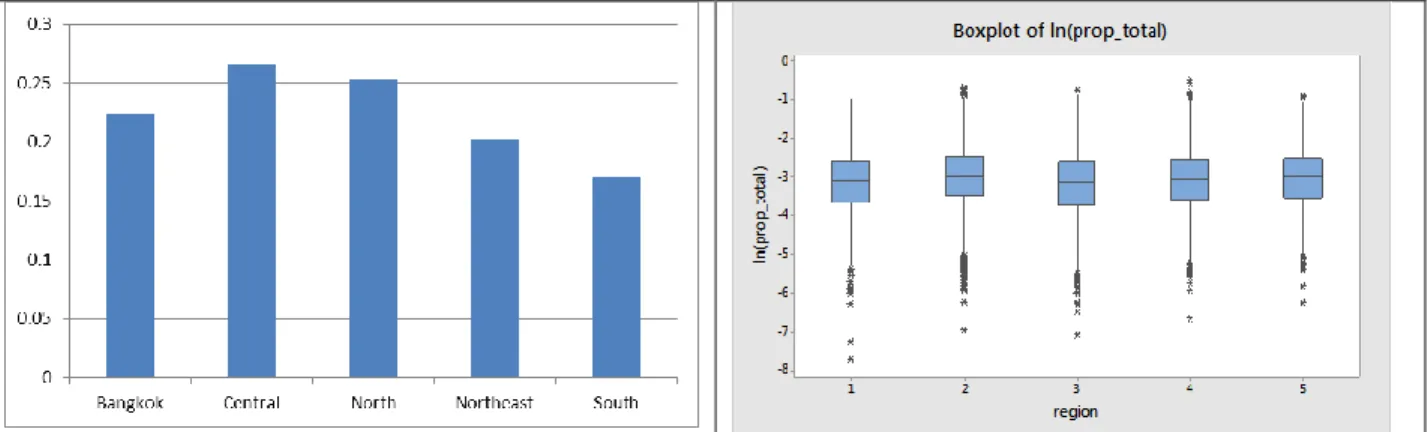
Figure 4: Proportions of non-zero drinking expenditures and box plots (for drinkers) of the (logged) proportion of total alcohol expenditure by region.
Figure 4 reveals a lower propensity to drink among Southern households, but not much regional differences in alcohol expenditure proportions for drinking households.
11
3. Logistic Regression Analysis
For the first analysis, we used logistic regression analysis to investigate the associations between alcohol consumption and demographic factors, tobacco expenditure, and gambling expenditure. We studied total alcohol consumption, alcohol consumption at home, and alcohol consumption away from home separately, as we think it is likely that these three types of consumption differ in terms of the relationships between the factors. Therefore, we analyzed three logistic regression models in this study. The responses for the three models refer to whether the household consumed alcohol in 2009, whether the household consumed alcohol at home in 2009, and whether the household consumed alcohol away from home in 2009, respectively. The factors for the three logistic regression models are all included in Table 2 with the exception of the last two factors, i.e., the proportion of tobacco expenditure and the proportion of gambling expenditure. The results of the three logistic regression models are shown in Table 2.
In summary, the results of the logistic regression suggest that the probability of consuming alcohol at home is higher for households in non-municipal areas (compared to municipal areas), in the central region (Bangkok excluded) (compared to the other regions), with a male household head (compared to female household head), with higher income, with a younger household head, with higher tobacco expenditure, with higher gambling expenditure, with a household head who has lower educational level, with a household head who is Buddhist (compared to households with a Muslim or other religion head), with a married household head, with a head with active work status. Based on the values of Chi-square, the strongest predictor of household that consumes alcohol at home is tobacco expenditure, followed by religion of a household head and sex of a household head. The results show that households with a household
12
head who is Buddhist is 14 times more likely to consume alcohol at home than the households with a household head who is Islamic, households with male household head are about twice more likely to consume alcohol at home than the households with female household heads.
Table 2: Logistic Regression Models for Total Consumption, Consumption at Home, and Consumption Away from Home
Total consumption Consumption at home
Consumption away from home coefficient (odds ratio) Chi-square (p-value) coefficient (odds ratio) Chi-square (p-value) coefficient (odds ratio) Chi-square (p-value) constant -0.641 -1.182 -1.756 number_household 0.10261 161.89 (0.000) 0.10547 (0.000) 134.43 0.0775 (0.000) 49.09 income 0.000001 3.54 (0.060) 0.000001 4.23 (0.040) 0.000001 4.52 (0.033) age -0.01987 266.12 (0.000) -0.02012 209.83 (0.000) -0.01322 61.31 (0.000) tobacco_expenditure 0.001134 978.34 (0.000) 0.000948 645.32 (0.000) 0.000686 256.04 (0.000) gambling_expenditure 0.000216 86.09 (0.000) 0.00013 (0.000) 30.95 0.000152 (0.000) 36.52 region [ref: Bangkok] (0.000) 222.79 (0.000) 238.67 (0.000) 172.60 Central 0.2938 (1.3415) (1.3447) 0.2962 (1.1938) 0.1772 North 0.3877 (1.4737) (1.1052) 0.1 (2.0399) 0.7129 Northeast -0.0099 (0.9901) (0.7820) -0.2459 (1.4450) 0.3681 South -0.0695 (0.9328) (0.8465) -0.1666 (1.3404) 0.293 area [ref: Municipal] (0.000) 18.51 (0.000) 27.44 (0.233) 1.42 Non-municipal 0.1142 (1.1210) (1.1714) 0.1582 (1.0449) 0.0439 sex [ref: Male] 551.16 (0.000) 311.72 (0.000) 265.83 (0.000) Female -0.7495 (0.4726) (0.5203) -0.6534 (0.4799) -0.7342 marital_status [ref: Single] 14.49 (0.002) 27.30 (0.000) 57.22 (0.000) Married 0.0925 (1.0969) 0.2887 (1.3347) -0.3403 (0.7116) Widowed 0.232 (1.2612) 0.2674 (1.3065) 0.0411 (1.0419) Other 0.0721 (1.0747) 0.1262 (1.1345) -0.0817 (0.9215) education
[ref: Missing values]
87.07 (0.000) 88.75 (0.000) 23.84 (0.002) Primary -0.1381 (0.8710) -0.1075 (0.8981) -0.1052 (0.9002) Lower_secondary -0.2789 (0.7566) -0.2152 (0.8063) -0.2667 (0.7659)
13 Upper_secondary -0.3883 (0.6782) -0.2961 (0.7437) -0.3161 (0.7290) Post_secondary -0.4117 (0.6625) -0.457 (0.6333) -0.164 (0.8487) Bachelor -0.4988 (0.6073) -0.5678 (0.5668) -0.249 (0.7797) Master -0.689 (0.5018) -0.828 (0.4369) -0.31 (0.7338) Doctoral -0.908 (0.4032) -1.54 (0.2139) 0.118 (1.1247) Other -0.465 (0.6284) 0.029 (1.0292) -1.341 (0.2616) religion [ref: Buddhist] 695.87 (0.000) 470.75 (0.000) 248.57 (0.000) Islamic -2.82 (0.0596) -2.658 (0.0701) -2.492 (0.0827) Other -0.417 (0.6588) -0.481 (0.6179) -0.247 (0.7809) work_status_original [ref: Employer] 231.34 (0.000) 91.89 (0.000) 180.15 (0.000) Own-account_worker -0.1228 (0.8844) -0.028 (0.9724) -0.2411 (0.7858) Family_worker -0.0172 (0.9829) 0.134 (1.1433) -0.323 (0.7237) Government_employee 0.3353 (1.3983) 0.192 (1.2117) 0.3861 (1.4712) State_enterprise 0.526 (1.6925) 0.389 (1.4756) 0.411 (1.5088) Private_company 0.2075 (1.2306) 0.204 (1.2263) 0.0968 (1.1017) Producers_cooperative -0.563 (0.5693) (0.4653) -0.77 (0.6694) -0.4 Housewife -0.0056 (0.9944) (0.9533) -0.0478 (1.0682) 0.066 Student -0.629 (0.5333) (0.5241) -0.646 (0.6053) -0.502 Child_elderly -0.2427 (0.7845) (0.8729) -0.1359 (0.6658) -0.4067 Ill_disabled -0.588 (0.5556) (0.5796) -0.545 (0.5419) -0.613 Looking_jobs -0.942 (0.3900) (0.5293) -0.636 (0.1883) -1.67 Unemployed -0.1 (0.9049) (0.7840) -0.243 (0.9904) -0.01 Other -0.221 (0.8019) (0.9237) -0.079 (0.6386) -0.449 amount_debt 0 0.03 (0.862) 0 (0.983) 0 0 (0.528) 0.40 disability [ref: No] 4.42 (0.036) 0.67 (0.415) 4.05 (0.044) Yes -0.1937 (0.8239) (0.9167) -0.087 (0.7680) -0.264 welfare [ref: No] 0.81 (0.367) 0.07 (0.786) 1.05 (0.307) Yes 0.0794 (1.0827) 0.0265 (1.0268) 0.129 (1.1374) government fund [ref: No] 0.18 (0.674) 0.02 (0.886) 0.85 (0.358) Yes 0.0142 (1.0143) 0.0055 (1.0055) 0.0429 (1.0439)
14
The probability of consuming alcohol away from home is higher for households in non-municipal areas (compared to non-municipal areas), in the North (compared to the other regions), with a male household head (compared to female household head), with higher income, with a younger household head, with higher tobacco expenditure, with higher gambling expenditure, with a household head who is Buddhist (compared to households with a Muslim or other religion head), with a widowed household head, with a household head with active work status. On the other hand, the probability of consuming alcohol away from home is lower for households with a disabled household head. Based on the values of Chi-square, the strongest predictor of household that consumes alcohol away from home is sex of a household head, followed by tobacco expenditure and religion of a household head. Similar to the alcohol consumption at home, the results show that households with a household head who is Buddhist is 12 times more likely to consume alcohol away home than the households with a household head who is Islamic, households with male household head are about twice more likely to consume alcohol away from home than the households with female household heads.
15
4. Treenet
In this section, we refine our understanding of alcohol consumption in the following way. Specifically, we applied data-mining models, which capture non-linearities and interactions automatically, to confirm or refute the effects discovered in the logistic model. For example, we are able to address the question of whether the logistic model overestimates the effect of having a Muslim head of household on the probability of that a household would engage in alcohol consumption.
In this second analysis, we investigated the association between the proportion of alcohol expenditure by total expenditure and demographic factors, tobacco expenditure, and gambling
expenditure. To demonstrate the techniques, we applied Treenet models (
www.salford-systems.com/treenet.html, Friedman, 2001) ( for the proportion of total expenditure spent on
alcohol, proportion of total expenditure spent on alcohol consumed at home, and proportion of total expenditure spent on alcohol consumed away from home separately. Accordingly, we constructed three models with different responses. The non-parametric approach adopted here makes it possible to handle a response variable with a large number of zero values (about 80% of the dataset).
Model 1: The response is the proportion of total expenditure spent on alcohol.
Model 2: The response is the proportion of total expenditure spent on alcohol consumed at home. Model 3: The response is the proportion of total expenditure spent on alcohol consumed away from home.
16
With the exceptions of tobacco expenditure and gambling expenditure which are replaced by their proportions to total expenditure, all the factors in Table 1 are included in each of the three Treenet models.
Figure 3 shows that four variables are important for predicting the proportion of total alcohol expenditure: the proportion of tobacco expenditure, the age of the head of household, the religion of the head of household, and the gender of the head of household.
Variable Score
PROP_TOBACCO 100.00 ||||||||||||||||||||||||||||||||||||||||||
AGE 50.82 |||||||||||||||||||||
RELIGION$ 41.21 |||||||||||||||||
SEX$ 41.05 |||||||||||||||||
Figure 3: Variable importance in the Treenet Model 1
Figure 4 (a-d) displays partial effects of each predictor on the estimated response (while holding other predictors constant). In Figure 4(a), we can see that the effect of the proportion of tobacco expenditure on the proportion of total alcohol expenditure “kicks in” at about an approximate value of 0.005, with no further effect beyond 0.005. These results suggest that a proportion of tobacco expenditure of 0.005 or above is associated with a jump in proportion of total alcohol expenditure of about 0.001 units. In Figure 4(b), we can see that estimated proportions of total alcohol expenditures do not depend on age until age reaches about 50, at which point they drop, to drop again after about 60 (ceteris paribus). Figure 4(c) reveals the negative effect of female gender (ceteris paribus), whereas Figure 4(d) reveals the negative effect of Muslim religion on the proportion of total alcohol expenditure (ceteris paribus).
17 Figure 4(a): Proportion of tobacco expenditure and proportion of total alcohol expenditure
Figure 4(b): Age and proportion of total alcohol expenditure
18 Figure 4(d): Sex and proportion of total alcohol expenditure
Figure 5 shows that five variables are important for explaining the proportion of alcohol expenditure consumed at home: proportion of tobacco expenditure, region of the household, sex of the head of household, proportion of gambling expenditure, and age of the head of household.
Variable Score PROP_TOBACCO 100.00 |||||||||||||||||||||||||||||||||||||||||| REGION$ 57.96 |||||||||||||||||||||||| SEX$ 35.00 |||||||||||||| PROP_GAMBLING 30.27 |||||||||||| AGE 29.68 ||||||||||||
Figure 5: Variable importance in Treenet Model 2
Figure 6(a) shows a similar pattern to that in in Figure 4(a). However, the trigger number is 0.001 instead of 0.005. Figure 6(b) shows the negative effect of regions 3 (North), 4 (Northeast) and 5 (South). Note that the effect of religion is probably captured by region since there is a high proportion of Muslim in the South of Thailand. Figure 6(c) reveals the negative effect of having a female head of household on the proportion of alcohol expenditure consumed at home. In Figure 6(d), we can see that the effect of the proportion of gambling expenditure on
19
the proportion of total alcohol expenditure “kicks in” at about an approximate value of 0.001, with no further effect beyond 0.001. These results suggest that a proportion of gambling expenditure of 0.001 or above is associated with a jump in proportion of total alcohol expenditure of about 0.00007 units. In Figure 6(e), the effect of age of the household head on proportion of alcohol expenditure consumed at home only appears when age reaches 50; at this age estimated home proportions drop and do not drop again at older ages.
Figure 6(a): Proportion of tobacco expenditure and proportion of alcohol expenditure consumed at home
20 Figure 6(c): Sex and proportion of alcohol expenditure consumed at home
Figure 6(d): Proportion of gambling expenditure and proportion of alcohol expenditure consumed at home
21
Figure 7 shows that five variables are important for predicting the proportion of alcohol expenditure consumed away from home: proportion of tobacco expenditure, work status of the head of household, sex of the head of household, proportion of gambling expenditure, and household income. Variable Score PROP_TOBACCO 100.00 |||||||||||||||||||||||||||||||||||||||||| WORK_STATUS$ 54.25 |||||||||||||||||||||| SEX$ 50.11 ||||||||||||||||||||| PROP_GAMBLING 47.37 ||||||||||||||||||| INCOME 37.70 ||||||||||||||| RELIGION$ 2.79 MARITAL_STATUS$ 2.11 AGE 2.06 NO_HOUSEHOLD 1.54
Figure 7: Variable importance in Treenet Model 3
Figure 8(a) shows a similar pattern to that in Figure 4(a). Figure 8(b) shows the positive effect of work status 4 (Government employees) and 5 (State enterprise employees), whereas Figure 8(c) shows the negative effect of having a female head of household on the proportion of alcohol expenditure consumed away from home. In Figure 4(d), we can see that the effect of the proportion of gambling expenditure on the proportion of total alcohol expenditure is like a step function. These results suggest that a proportion of gambling expenditure at about 0.001-0.002 is associated with a jump in proportion of total alcohol expenditure of about 0.000004 units. The first drop of 0.000001 units appears at about proportion of 0.01, the second drop of 0.0000005 units appears at about proportion of 0.025, and the third drop of 0.0000005 units appears at about proportion of 0.050. In Figure 4(a), we can see that the effect of monthly income on the proportion of total alcohol expenditure “kicks in” at about an approximate value of 62,500 Bahts considered a high income in Thailand (only 5.26 % of the dataset have income 62,500 Bahts and
22
above), with no further effect beyond this value. These results suggest that an income of 62,500 Bahts is associated with a jump in proportion of total alcohol expenditure of about 0.000007 units.
Figure 8(a): Proportion of tobacco expenditure and proportion of alcohol expenditure consumed away from home
23 Figure 8(c): Sex and proportion of alcohol expenditure consumed away from home
Figure 8(d): Proportion of gambling expenditure and proportion of alcohol expenditure consumed away from home
24
From all three models, the proportion of tobacco expenditure is the most important variable. The sex of the head of household is also an important variable for all the models, whereas the age of the head of household is an important variable for Models 1 and 2. The proportion of gambling expenditure is an important variable for Models 2 and 3. Religion of the head of household is an important variable for Model 1, whereas region (which acts as proxy for religion) is an important variable for Model 2. The work status of the head of household and income are important variables for Model 3. Interestingly, religion does not seem to be an important variable in Model 3; its effects are probably captured by those of gambling expenditures.
The Treenet results suggest that the proportion of total alcohol expenditure is higher for households that consume tobacco with proportion higher than 0.005, households whose head of household is younger than 50 years old, households with a male head of household, and households whose head of the household is non-Muslim. The proportion of expenditure on alcohol consumed at home is higher for households that consumed tobacco with proportion higher than 0.001, households whose head of household is younger than 50 years old, households in Bangkok and the central area, households with a male head of household, and households that spend money on gambling with proportion more than 0.001. The proportion of expenditure on alcohol consumed away from home is higher for households that consumed tobacco with proportion higher than 0.005, households with a male head of the household, households that spend money on gambling with proportion between 0.001 and 0.01, households whose head of household works for the government or is a state enterprise employee, and households with an income above 62,500 Thai Bahts.
25
5.
Directed Acyclic Graph (DAG)
In this section we construct a directed acyclic graph (AKA Bayesian network) to help unravel direct and indirect effects of household characteristics on alcohol expenditures. The importance of these techniques, highlighted by the recent (2011) Turing prize awarded to Judea Pearl, has been growing, along with the debate among researchers on whether traditional statistical models used in many applications carry enough evidence to warrant policy recommendations. The issue of causality is of course at stake here, and there is no claim to a conclusive answer (Pearl, 2009 and Spirtes, 2000). A number of algorithms exist for constructing DAGs, falling essentially into two categories: Constraint-based algorithms, such as the PC algorithm, and GS (Greedy Search; package bnlearn in R, see Scutari, 2010) and Score based algorithms (Conrady and Jouffe, 2015).
We employ an algorithm implemented by the Bayesialab software
(http://www.bayesia.com) Note that all variables were discretized in the Bayesialab implementation. We employed a Taboo search algorithm which is a greedy score-based algorithm. It allows to temporarily iterating to less optimal solutions with a smaller score in order to avoid being stuck near a local optimum in the search space.
It appears from Figure 9 that the proportions of expenditure on alcohol, tobacco and gambling are closely linked. The proportion of expenditure on alcohol has a direct effect on both the proportion of expenditure on tobacco and the proportion of gambling expenditure. If we force the proportion of expenditure on alcohol to be at a higher level (Figure 9b), the proportion of expenditure on gambling and the proportion of expenditure on tobacco will be higher as well. This result implies that higher household spending on alcohol will lead higher spending on tobacco and higher spending on gambling as well. The religion of the household head connects
26
to alcohol and tobacco only via region of the household which implies that the impact of religion on alcohol and tobacco operated via the geographical location of the household. On the other hand, the religion of the household head has a direct effect on gambling. The gender of the household head has a direct effect on both alcohol and tobacco. The age of the household head connects to alcohol via household size and marital status of the household head which implies that the effect of age of the household head on alcohol operates via depends on both two factors, namely whether the household head is single, married, widowed and how many people live in the household. The educational level of household head does not have a direct effect on alcohol, tobacco and gambling. However, it has an indirect effect thought several paths including via the income of the household and region of the household.
27 Figure 9b: Impact of interactions on the proportion of alcohol expenditures on gambling and tobacco proportions.
28
6. Conclusion
This paper provides a thorough study of alcohol consumption in Thailand in regard to the relationships between alcohol consumption, tobacco consumption, gambling consumption, and demographic factors. We applied three statistical models and data-mining techniques—logistic regression, Treenet, and DAG—to the analysis of datasets drawn from socio-economic surveys of 43,844 Thai households conducted in 2009. Beyond the bivariate analysis, multiple linear regression, and logistic regression analysis used in the literature related to the study of alcohol (e.g., Stinchfield (2000), Jackson et al. (2002), Wetzels et al. 2003, Duhig et al. (2007), Aekplakorn et al. (2008), Barnes et al. (2009), Bonevski et al. 2014), we also implemented new methods that had never been used in this context before: Treenet and directed acyclic graph (DAG). Treenet provides non-linear associations between response and predictors, whereas DAG analyzes direct and indirect effects between variables.
The results from our study show that alcohol, tobacco and gambling co-occur. Through logistic regression, the strongest predictors of household that consumes alcohol are tobacco expenditure, religion and sex of a household head. Through Treenet, we found that the proportion of tobacco expenditure is the most important predictor for proportional of alcohol expenditure. Moreover, the result from DAG shows that alcohol has a direct effect on both tobacco and gambling, i.e. the proportion of total expenditure a household spends on alcohol directly affects proportions spent on tobacco and on gambling. The gender of head of household has a direct effect on household alcohol spending (from DAG). The presence of a female household head is associated with a lower likelihood to consume alcohol and lower alcohol proportions spending (from logistic regression and Treenet). The religion of the household head is also associated with both alcohol consumption and spending. Households with a Muslim
29
household head have a lesser likelihood to consume alcohol and smaller alcohol spending proportions (from logistic regression and Treenet). However, through DAG, we found that the effect of religion on alcohol expenditure operates via the region of the household. This seems to suggest that community and geographical location play an important role here. The age of the household head is also related to alcohol consumption and spending. Households with a younger household head have a higher likelihood to consume alcohol and higher on alcohol spending proportions (from logistic regression and Treenet). However, through DAG, we found that the effect of age on alcohol expenditure operates via the marital status of the head, namely whether the household head is single, married, widowed and via household size. The educational level of household head is also associated with alcohol consumption. Households with a lower-educated household head have a higher likelihood to consume than households with a higher-educated household head (from logistic regression). However, from DAG, we found that the educational level of the household head does not have a direct effect on the proportion of alcohol expenditure. It has an indirect effect thought several paths including income of the household and region of the household. Regarding work status, both logistic regression and Treenet models show that households with a household head who is a government employee or state enterprise employee has a higher likelihood to consume alcohol and higher alcohol spending proportions. This is surprising since government employees generally have lower income than those with other work status, e.g. employer and private company employee.
With all the associations, direct and indirect effects from our study, we expect our results to be useful to both researchers and government practitioners in their efforts to tailor programs to target households that include alcohol-dependent members in order to reduce problems related to alcohol consumption in Thailand.
30
Acknowledgement
We would like to thank Dr. Robin Room, an editor of Drug and Alcohol review, for his guidance in interpreting and communicating the results to the readers, and his thorough advice in revising this paper.
References
1. Aekplakorn W., Hogan, M. C., Tiptaradol, S., Wibulpolprasert, S., Punyaratabunduhu, P., Lim, S. S. (2008). Tobacco and hazardous or harmful alcohol use in Thailand: Joint prevalence and associations with socioeconomic factors, Addictive Behavior (33), 503-514.
2. Agresti, A. (2002). Categorical Data Analysis (2nd ed.) (New Jersey: Wiley).
3. Assanangkornchai, S., Onigrave, K. M. & Saunders, J. B. (2002). Religious beliefs and practice, and alcohol use in Thai men. Alcohol and Alcoholism, 37(2), 193-197.
4. Assanangkornchai, S., Sam-Angsri, N., Rerngpongpan, S., Lertnakorn, A. (2010). Patterns of Alcohol Consumption in the Thai Population: Results of the National Household Survey of 2007. Alcohol and Alcoholism, 45(3), 278-285.
5. Assanangkornchai, S., Geater, A. F., Saunders, J. B. & McNeil, D.R. (2002). Effects of paternal drinking, conduct disorder and childhood home environment on the development of alcohol use disorders in a Thai population, Addiction, 97(2), 217-226.
6. Barnes, G. M., Welte, J. W., Hoffman, J. H., et al. (2009). Gambling alcohol, and other substance use among youth in the United States. J Stud Alcohol Drugs, 70, 134–142. 7. Bonevski B., Regan T., Paul C., Baker A. L., Bisquera A. (2014). Associations between
alcohol, smoking, socioeconomic status and comorbidities: evidence from the 45 and Up Study. Drug and Alcohol Review, 33(2), 169-176.
8. Burger, M., Mensink, G., Bronstrup, A., Thierfelder, W. & Pietrzik, K. (2004). Alcohol consumption and its relation to cardiovascular risk factors in Germany. Eur J Clin Nutr, 58, 605–614.
9. Chiolero, A., Wietlisbach, V., Ruffieux, C., Paccaud, F., Cornuz, J. (2006). Clustering of risk behaviors with cigarette consumption: A population-based survey. Prev Med, 42, 348–353.
10. Clausen, T, Charlton, K. E., Holmboe-Ottesen, G. (2006). Nutritional status, tobacco use and alcohol consumption of older persons in Botswana. The journal of nutrition, health &
aging, 10, 104–110.
11. Conrady, S. & Jouffe, L. (2015). Bayesian Networks and BayesiaLab: A Practical
31
12. Duhig, A. M., Maciejewski, P. K., Desai, R. A., et al. (2007). Characteristics of adolescent past-year gamblers and non-gamblers in relation to alcohol drinking. Addict
Behav, 32, 80–89.
13. Friedman, J. (2001). Greedy Function Approximation: A Gradient Boosting Machine,
The Annals of Statistics, 29(5), 1189-1232.
14. Jackson, K. M., Sher, K. J., Cooper, M. L. & Wood, P. K. (2002). Adolescent alcohol and tobacco use: onset, persistence and trajectories of use across two samples. Addiction, 97, 517–531.
15. Kahler, C. W., Strong, D. R., Papandonatos, G. D., Colby, S. M., Clark, M. A., Boergers, J., Niaura, R., Abrams & D. B., Buka, S. L. (2008). Cigarette smoking and the lifetime alcohol involvement continuum. Drug Alcohol Depend, 93, 111–120.
16. Kamsa-ard, S., Promthet, S., Lewington, S., Burrett, J. A., Sherliker, P., Kamsa-ard, S.,
Suwanrungruang, K. & Parkin, D. M.(2014). Alcohol Consumption and Mortality: The
Khon Kaen Cohort Study, Thailand, Journal of Epidemiology, 24(2), 154–160.
17. Kasantikul, V., Ouellet, J. V., Smith, T., Sirathranont, J., & nichabhongse, V. (2005). The role of alcohol in Thailand motorcycle crashes. Accident Analysis & Prevention, 37(2), 357–366.
18. Peters, E. N., Nordeck, C., Zanetti, G., O’Grady, K. E., Serpelloni, G., Rimondo, C., Blanco, C., Welsh, C. & Schwartz, R. P. (2015). Relationship of gambling with tobacco, alcohol, and illicit drug use among adolescents in the USA: Review of the literature 2000-2014 American Journal on Addition, 24, 206–216.
19. Puangsuwan, A., Phakdeesettakun, K., Thamarangsi, T., Chaiyasong, S. (2012). Compliance of off-premise alcohol retailers with the minimum purchase age law. WHO
South-East Asia Journal of Public Health, 1(4), 412-422.
20. Scutari, M. (2010). Learning Bayesian Networks with the bnlearn R Package. Journal of Statistical Software, 35(3), 1-22.
21. Sornpaisarn, B., Shield, K.D. & Rehm, J. (2012). Alcohol taxation policy in Thailand: Implications for other low- to middle-income countries, Addiction, 107 (8), 1372-1384.
22. Spirtes, P., Glymour, C., & Scheines, R. (2000). Causation, Prediction, and Search, 2nd
edition. MIT Press, Cambridge MA.
23. Stinchfield, R. A. (2010). Critical review of adolescent problem gambling assessment instruments. Int J Adolesc Med Health, 22, 77–93.
24. Thamarangsi, T. (2006). Thailand: alcohol today. Addiction, 101 (6), 783-787.
25. Thavorncharoensap, M., Teerawattananon, Y., Yothas amut, J., Lertpitakpong, C., Thitiboonsuwan, K. & Neramitpitagkul, P. (2010). The economic costs of alcohol consumption in Thailand, BMC Public Health, 10, 323.
26. Wetzels, J. J., Kremers, S. P., Vitoria, P. D., de Vries, H. (2003). The alcohol-tobacco relationship: a prospective study among adolescents in six European countries. Addiction, 98, 1755–1763.
27. Woratanarat, P., Ingsathit, A., Suriyawongpaisal, P., Rattanasiri, S., Chatchaipun, P., Wattayakorn, K. & Anukarahanonta, T. (2009). Alcohol, illicit and non-illicit
32
psychoactive drug use and road traffic injury in Thailand: a case-control study. Accident
Analysis Prevention, 41(3), 651-657.
29. Pearl, J. (2009). Causal Inference in Statistics: An Overview. Statistics Surveys, 3, 96-146.