HAL Id: halshs-00564839
https://halshs.archives-ouvertes.fr/halshs-00564839
Preprint submitted on 10 Feb 2011
HAL is a multi-disciplinary open access
archive for the deposit and dissemination of sci-entific research documents, whether they are pub-lished or not. The documents may come from teaching and research institutions in France or abroad, or from public or private research centers.
L’archive ouverte pluridisciplinaire HAL, est destinée au dépôt et à la diffusion de documents scientifiques de niveau recherche, publiés ou non, émanant des établissements d’enseignement et de recherche français ou étrangers, des laboratoires publics ou privés.
Credit constraints and distance, what room for Central
banking? The French experience (1880-1913)
Guillaume Bazot
To cite this version:
Guillaume Bazot. Credit constraints and distance, what room for Central banking? The French experience (1880-1913). 2010. �halshs-00564839�
WORKING PAPER N° 2010 - 08
Credit constraints and distance,
what room for central banking?
The French experience (1880-1913)
Guillaume Bazot
JEL Codes: D43, D82, E58, G21, N13, N23, R51, R58 Keywords: Credit constraint, credit development, local banking, soft information and central bank branches
P
ARIS-
JOURDANS
CIENCESE
CONOMIQUES48,BD JOURDAN –E.N.S.–75014PARIS TÉL. :33(0)143136300 – FAX :33(0)143136310
www.pse.ens.fr
CENTRE NATIONAL DE LA RECHERCHE SCIENTIFIQUE –ECOLE DES HAUTES ETUDES EN SCIENCES SOCIALES ÉCOLE DES PONTS PARISTECH –ECOLE NORMALE SUPÉRIEURE –INSTITUT NATIONAL DE LA RECHERCHE AGRONOMIQUE
Credit Constraints and Distance, What
Room for Central Banking? The French
Experience (1880-1913)
Guillaume Bazot Paris School of Economics1
bazot@pse.ens.fr March 2010
JEL Class: E58, G21, N13, N23, R51, R58
Credit Constraints and Distance, What Room for
Central Banking? The French Experience (1880-1913).
Abstract
Although a relative consensus is emerging about the economic effec s of credit development, many controversies remain as to the role of the central bank in that development. This pape addresses the process of credit allocation by the central bank as observed on a spatial basis. It examines how and why improved geographical access to the central bank contributes to redit development by looking at the F ench experience in the ‘classical period’ (1880-1913). n an environment of emerging, but highly prudent, d posit banks and the absence of a centralised money market, Banque de F ance branches had enough supply and demand to generate a network. Access to “central loans” hence r duced liquidity constraints and encouraged local banks and firms to lend. We shape the proof in two stages. First, a simple banking mod l presents our intuition and the mechanisms at work. Second, we take a new data set on the development of credit by French geographic area (départemen ) to test our hyp thesis using panel econometric tools. The results show the Banque d France branches having a strong and robust impact on credit development. t r c r I e r e e t o e
Central banking is not the job of a single man deciding merely to change interest rates or the quantity of money in a given period of the economic cycle. It is also a microeconomic position used to gather information from local areas and local banking institutions. Central banks therefore often have a complex network of local branches all working on improving their knowledge of local businesses. Basically, understanding how businesses tick helps central banks bring funds to local players and relax credit constraints. Yet such a network is not always necessary and its optimal size may differ, depending on the central bank’s objective and the organisation of the money market. The French case is particularly interesting from this point of view, since the Banque de France played an important role in national money market integration and developed a large network of branches in the late 19th century.
The Banque de France branches (Banque branches) were major French banking system players at the beginning of the twentieth century. By 1911, more than 180 branches2 discounted or rediscounted almost 40% of all bills created in France. Size, however, was not necessarily a good thing. For example, Bank of England branches were not without their critics (see Clapham, 1944). Some feared that the Bank of England branches’ use of their privileges might crowd out other banking institutions, reducing banking competition and restricting credit, especially to non-strategic sectors. Aversion to government intervention, the adoption of the ‘currency 2 Banque branches plus Banque sub-branches.
principle’ and fears of competitive distortions were thus the main arguments against the establishment of Bank of England branches. In addition, detractors argued that too many branches could be counterproductive for the Bank. For instance, the Bank of England used the gold in its vault to grant liquidity through the English banking system’s pyramid structure and open market operations. So the Bank provided money through the discount houses, which redistributed it nationwide. The organised and structured money market hence did away with the need for expensive branches and large stocks of gold.
The French monetary system was prevented from importing the English system’s characteristics due to a young, non-hierarchical banking structure outside the largest cities (Levy-Leboyer, 1979). A central banking network was thus a logical alternative, as shown in a recent paper on the Japanese experience (Mitchener & Ohnuki, 2009). Furthermore, local branches could solve some information issues and generate positive externalities. The Banque could, for example, provide liquidity to the economy either directly or through the intermediation of local banks. In other words, the use of local information meant that the Banque branches could improve credit conditions in many small business areas where there were complaints about a lack of liquidity. In this respect, Banque branches rarely overlapped with local banking businesses.
The Banque de France branches were consequently a crucial element of French economic policy. In addition to filling the gap historically filled by the market in the English case, the Banque branches were used to promoting credit development nationwide. The question then is whether positive effects outweigh negative ones.
We answer this question using a new data set on credit supply by French geographic area (département). To this end, we have collected information on bills issued in 1881, 1891 and 1911 by taking the amount of stamp duty reported in the Bulletin de Statistique et de Legislation Comparée and evaluated by G. Rouleau (1914). As this duty was on all kinds of bills (“effets de commerce”), proportional to their face value, it is the perfect way to evaluate the amount of credit.
Our evaluation is made up of three main steps. We first build a basic model explaining how the Banque branches could reduce credit constraints. Second, we ask whether the Banque branches increased credit development. Third, since the Banque is a private institution, some of its choices were motivated by profit maximisation. Identification issues therefore prevent our variable from being totally exogenous. We thus use instrumental variable estimations to eliminate the bias. Given the strong political pressure brought to bear on the Banque, the relative size of the largest cities is a good instrumentation method. Consequently, the IVs used are the share of population in the département’s number one and number two cities. Although all the indicators bear out our instrumentation strategy, we also
use the difference between both ratios to dissipate any doubt as to the expected effect of development on city size.
Basically, all results converge to establish the positive effect of the Banque network. Yet what mechanisms are at work? Let’s assume trade credit (the most common in this period). The information gap means that the Banque branches refuse to rediscount distant banks’ bills. These banks have to put reserves in their vaults to avoid liquidity constraints. Their credit to the economy is thus reduced proportionally by the amount of these reserves. Assume a new Banque branch is set up now. This new Banque branch rediscounts new bills from previously excluded banks. These banks’ supply increases automatically by the amount of their previous reserves. Since the merchants are thereafter sure to avoid liquidity constraints, they are encouraged to draft new commercial bills. In other words, the amount of credit to the economy grows proportionate to the banks’ previous reserves.
Looking at robustness, the regional panel rules out some institutional bias. Since the legal institutions (i.e. bankruptcy law) are roughly the same in every French département, the econometric specifications are not undermined by a lack of basic institutional variables. This point is a common shortcoming in cross-country models.
Furthermore, although we focus on the French case, this issue has wider reaching significance. For instance, a number of developing economies have similar structures today. The results could thus be extended to financially decentralised economies where the local banks are important players.
Since the local banks had more of a capacity to finance investment than the deposit banks (see Nishimura, 1995, and Lescure, 2009), the protection offered by the Banque may well have prompted a better allocation of capital. Therefore, the French central banking policy was probably efficient at promoting innovation and growth (Bazot, 2010, finds evidence of the establishment of Banque branches having a positive impact in terms of the effects of local banking on innovation and GDP growth).
The first section of the paper looks at the historical background. Section II discusses the theoretical analysis. Section III presents the data on credit development. Section IV looks at the basic econometric specification and results. Section V proposes robustness checks. Section VI discusses some points further. Section VII concludes.
I. Historical Background
The French banking system at the end of the 19th century was a combination of three major players3: private banks, deposit banks (Crédit
3 Notaries and Crédit Foncier could be added into this typology, but they do not tie in with the topic we are addressing here.
Lyonnais, Société Générale, Comptoir National d’Escompte and Credit Industriel et Commercial) and the Banque de France. What was their place in the credit process?
Local banks were the biggest suppliers of credit through to WWI. Estimates from Bouvier (1979) find they held 70% of the discount market up to the end of the 19th century. Local banks had, however, to deal with growing constraints due to competition from deposit banks. This indeed seems to tie in with the gradual backslide in their business. As shown by our tests,4 if the number of deposit bank branches per capita rises by 1 point,5 the number of local bank branches per capita decreases by 0.48 points (see Table 7 in the appendix). Given the average variation in the former (=0.02), the latter decreases on average by 0.01 points. Since the latter posted an average of 0.06 points in 1880, 17% of local bank branches collapsed under the pressure of competition from deposit banks. Not surprisingly, the share of local bank branches in France fell from 91% in 1880 to 66% in 1910. All in all, the number of local bank branches decreased 5% from 2,017 in 1881 to 1,914 in 1911.
Local banks had such a wide range of activities that it is hard to give a uniform presentation of them. They might have been single branch banks or multi-branch banks spread over quite a small area (the French literature talks about regional banks). It is, however, possible to pool some common features. To this end, Nishimura (1995), Plessis (2001) and monographs (see, for instance, Moine 2001) provide us with valuable information. Local banks operated in specific areas delimited by specific industries or businesses. They often used their private knowledge to reduce information asymmetries. In other words, they worked with regular clients whose behaviour and activities they knew well. Their loans were not limited to basic discounts. As argued by Nishimura (1995), complex devices were used to provide medium-term and long-term loans. This was especially true in industrial areas after 1890 (i.e. Longwy, Grenoble, Nancy and Lille).
To sum up, local banks were in a better position to be able to provide riskier, long-term funds due to their private knowledge of the firms in the business areas where they operated. In this respect, they were probably more similar to German banks than French deposit banks. However, this aspect was an obstacle to their borrowing on the money market. Local banks had thus to deal with a routine liquidity risk. This is the reason why they appealed to the Banque de France branches for assistance. Also, demand peaked with the threat of deposit bank competition.
Conversely, deposit banks opted for secure activities and often competed with the Banque. They captured short-term deposits and were consequently prompted to supply “safe”, short-term, liquid credits. On the
4 We only used the fixed effect results found by the Hausman test. 5 In thousands of inhabitants.
other hand, their hierarchical structure drove them to deal in common discount transactions. Information was thereby easily transferred from branches to headquarters (see Stein, 2002, for theoretical evidence). However, their strategy prevented them from discounting ambiguous bills from (risky) local areas.
Not unconnected with its macroeconomic policy, the Banque de France had major microeconomic operations in the local money markets. A decentralised banking system through to the last quarter of the 19th century (see Levy Leboyer, 1979) meant that banking institutions were unable to spread liquidities throughout the country. The Banque de France had to therefore carry the money market’s imperfections6. Three goals were traditionally assigned the Banque: to promote the nationwide integration of the financial markets, to reduce interest rates and to facilitate access to credit. Banque branches were the perfect tool to meet these aims since the network set-up meant that surplus could be removed from one region to meet the financial needs of other regions.
The size of the Banque’s network can be deduced from a number of facts. First, in return for the monopoly of note issue granted the Banque in 1857, the government pressed it to set up a Banque branch in every French département. When the monopoly was renewed in 1897, the Banque had to set up new Banque branches in every “prefecture” along with 30 Banque sub-branches. So the sum of those commitments concerned 129 branches, 87 of which appearing because of this.
Second, as the Banque was a private institution, profit maximisation triggered some new branches7. This was particularly the case in the 1890s when the deposit banks expanded their activities. The resulting competition on safe bills reduced the Banque branches’ profits and drove them away from their usual activities. Our evaluation finds that the average area’s Banque branch profits decreased by 1.2% as the share of deposit bank branches rose by 1%. Since the variation in this share was 27% on average, deposit bank competition reduced the Banque branches’ profits by 34% (see Table 8 in the appendix). As a result, the Banque changed its strategy and redeployed its businesses on a more regional manner. It also chose to work with previously ignored local bankers whose demand of liquidity was high8. As evidence of this, the regressions in Table 8 show a positive correlation between the number of Banque branches and profits per département given the Banque loans per département.
Third, in addition to the action of politicians (MPs and ministers), local lobbies (especially local banks) pressured the Banque to set up new
6 This confirms Gershenkron’s point of view about the role of large organisations in the development process of backward economies.
7 See, for instance, the Banque Branch Committee report of 10 September 1908 on the establishment of the Bethume sub-branch.
8 Especially because of deposit bank competition as mentioned above.
7 Banque branches. The case of Cherbourg is typical. The Banque branch committee report of 30 May 1882 speaks of “highly active approaches” by Cherbourg’s municipality. Furthermore, this report gives evidence of the personal involvement of the finance minister. Also, the electoral map meant that the largest city in each département stood more of a chance of getting the politicians’ support.
However, why did cities ask for Banque branches? As mentioned above, the growing market share taken by deposit banks reduced the local banks’ activities. In this respect, it became harder for “unsound” firms to access liquidity. Consequently, many banks and firms depended on the Banque to rediscount. Nevertheless, the lack of information constrained the Banque branches to provide services to local players only. Distance was therefore a major element of liquidity constraint. Some examples confirm this point. For instance, the Banque branch committee report of 30 May 1882 mentions the establishment of a Banque branch in Cherbourg: “The distance from St Lo (the nearest Banque branch) and differences in the nature of the transactions rule out any prejudice from the latter against the former”. The report adds, “St Lo’s portfolio does not have more than FF 200,000 of Cherbourg’s paper”. Lastly, it says, “Cherbourg’s Banque branch allows for contact to be made with two other banks in Valognes,” (a large city in the département close to Cherbourg) “which did not work with the Banque yet”.
The fourth size element is that the end of the bimetallist system in 1876 put the Banque in a very comfortable situation (see Flandreau, 1996). Although silver coins were not in circulation anymore, the Banque could still legally reimburse its paper money using this metal. The Banque could thus push back the bullion point from which gold escapes. The Mundell ‘trilemma’ was somehow averted, which gave monetary policy space in spite of the gold standard and international capital mobility. Consequently, international monetary events did not prevent the Banque’s expansionist action on the national market. Thereafter, the related formation of metal provisions in the late 19th century gave the Banque the opportunity to take a more active position in the banking system.
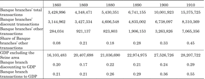
All these facts led the Banque to position itself as central banker (see Lescure, 2003) to improve credit conditions nationwide. Empirical analyses give evidence of this hypothesis. First, while the Banque’s discount curve was in line with the economic cycle up to 1890, it tended to be countercyclical from 1890 through to the war (Baubeau, 2004). Second, the number of Banque branch transactions rose faster than GDP from 1890 to 1914 (Graph 1, Table 1).
Table 1: Banque transactions
In tens of thousands of Francs
1860 1869 1880 1890 1900 1910
Banque branches’ total
transactions 3,428,996 4,348,471 5,430,351 6,741,155 10,001,923 15,375,725
Banque branches’
discount transactions 3,144,962 3,427,334 4,606,548 4,835,002 6,738,097 8,310,369 Banque branches’ other
transactions 284,034 921,137 823,803 1,906,153 3,263,826 7,065,356 Share of Banque branches’ other transactions 0.08 0.21 0.18 0.28 0.33 0.45 GDP excluding the Seine area 16,103,483 20,407,698 21,036,690 22,974,975 27,526,726 28,207,722 Banque branch discounting to GDP 0.20 0.17 0.22 0.21 0.24 0.29 Banque branch transactions to GDP 0.21 0.21 0.26 0.29 0.36 0.55
Sources: Reports to Banque de France shareholders
Graph 1: Economic share of Banque branches’ activities
On other hand, Banque branch transactions were particularly useful to local bankers. Lescure (2003) reports that the rediscount portfolio was made up of 83% of local bank bills in 1880 and 1910. This “marriage” was purely the result of circumstances. With the rise of the deposit banks, while the Banque needed to find new businesses, local banks loudly asked for Banque branches. Supply and demand were there to celebrate the union.
Finally, new central banking activities made it easier to rediscount accommodation papers and low-value papers (Nishimura estimated accommodation papers at 6.5% of the total rediscount figure). The Banque became more democratic, decentralised and diversified.
However, did the Banque’s active local stance bring credit development about? What mechanisms were actually at work? Did general equilibrium effects offset the Banque’s action? A comparison of départements combined with a microeconomic analysis can help answer those questions.
II. Credit supply and the Banque branch network
Recent microeconomic banking literature gives evidence of the effects of distance on credit constraints. For instance, Petersen & Rajan (2002) prove that physical distance in the United States reduces the capacity for lending to small, opaque firms, although this effect wanes with progress in information and communication. For Berger & DeYoung (2006), the cost and profit efficiency of multi-branch banks decreases with physical distance from the parent bank. Also, Alessandrini et al. (2006) find that small firms suffer from both cultural and physical distance on a sliding scale with the share of banks headquartered in the distant province.
Basically, where contracts entail local knowledge, close ties help tackle the information asymmetry. Since distance and the quality of information are closely linked, better geographical access improves the ability to lend. From this respect, the greater the distance, the greater the cost of capital allocation.
This point is especially true of our subject in this paper. Given the economic weight of local businesses and industrial districts, the information often stayed out. For instance, a lack of tools traditionally used today (homogeneous balance sheet (see Lemarchand, 1996) and systematic data) prevented outsiders from doing business.
The French credit system was widely built on the bill device. Let’s present the basic case. To begin with, a producer issues a bill to a client. If the creditor needs liquidity, he applies to a bank to rediscount the bill. If the quality of the producer and/or the client is/are recognised as good enough by the bank, funds are lent. The bank waits the client’s repayment on the settlement date. If the client fails to pay, the bank goes back to the producer.
The bank was able to issue other bills directly, through advance on account for instance. Such credits were, however, riskier since the bank could rely on neither producer awareness nor joint liability. The bank therefore needed to be sure of the quality of its client, which called for substantial private knowledge.
The Banque de France used the discount process to provide liquidity to banks and firms alike. Banque branches rediscounted countersigned, good quality bills (as proved by the rating system used in all Banque branches). In addition, to prevent an information gap, banks and firms needed to be known to and close to the Banque branch. So rediscounting could not be done by distant Banque branches.
Through this process, Banque branches helped to reduce local players’ liquidity constraints. Consequently, local players stood more of a chance of securing credit to protect them from liquidity constraints. They were thus encouraged to issue more bills, which automatically drove up the volume of credit. In summary, the Banque de France’s many branches made for greater access to liquidity, which probably increased the availability of credit nationwide.
Let’s take the example of a region (here Picardie) and mark the reach of Banque knowledge on the map. Within the zone, Banque branches can rediscount bills.
In this scenario, a small part of the region is covered by Banque knowledge. Therefore, local banks outside the zone are liquidity constrained (note that two areas are marked as knowledge quality deteriorates with distance).
Imagine that a new Banque branch is set up now. A new information zone is drawn on the map. Logically speaking, Banque knowledge improves. Other banks and firms are henceforth able to rediscount their bills. Local players are also less constrained by the lack of liquidity, which improves credit opportunities. Eventually, the amount of credit grows.
An easy model helps explain the intuition here. Let’s take, for the sake of simplicity, a trade credit economy. A bank far from any Banque branch is denoted at t=0, where the bank is unable to rediscount any bills. At t=1, a new Banque branch is set up. Now the bank can rediscount its safe bills at interest cost î. There are two kinds of bills: safe9 and unsafe10. Safe bills are those that are easy to rediscount. All the others are defined as unsafe bills. Credit constraints are such that demand for funds is always greater than the bank’s capacity11.
In a profit maximisation process, the bank chooses its efficient portfolios in both periods. At t=0, the bank determines an amount of reserves (R) to protect itself against the risk of illiquidity. R is thus a
9 In this case, commercial bills are a good example of safe bills. 10 Advance on account, for instance.
11 This hypothesis is always true in this period (see Bouvier 1979 for evidence).
function of the aggregate risk of all credit. At t=1, this risk is mitigated by the amount of safe ‘rediscountable’ credit provided by the bank. Nevertheless, the bank chooses this strategy if î is small enough to secure higher profits than at t=0. Therefore, if demand from safe clients is high enough, the bank substitutes all its previous reserves. Reserves fall to zero (R=0). The bank consequently raises the volume of its credit by an amount exactly equal to R.
These hypotheses are clearly borne out by monographs (see, for instance, Moine, 1999) and Banque archives12. For example, the minutes of the Banque branch committee meeting state, “Bankers are not less desirous than people. (…) Unforeseeable demand for money from their depositor obliges them to keep unproductive funds in their vaults. Such immobilisations will disappear with the ability to get immediate liquid assets on presentation of their [safe] bills to the Banque rediscount office.” As soon as the Banque branch opens, banks substitute their ‘extra’ reserves with ‘rediscountable’ bills.
Eventually, a firm issues bills if a bank is able to discount them. Therefore, if the volume of credit increases at t=1, firms are less reluctant to provide trade credit to their clients. Let ζ(L) be the volume of bills supplied by the firm and L be access to liquidity. We know that:
∆L= f(R) (1) If C is the amount of credit, ∆C=∆Lζ(L). Under (1), the amount of
new credit generated by the new Banque branch is:
∆C =ζ(f(R))>0 (2) In other words, the amount of credit increases proportionate to R. Moreover, if the elasticity of C to R is greater than one, the Banque branch rediscount amount is lower than ∆C. This situation corresponds to the credit multiplication effect. In this case, the Banque branch is plays an extremely important role in the development of local credit.
In this simple model, we have to collect accurate local information on credit to empirically gauge the effect of the Banque network. To this end, we have built new data on bills issued by French département.
III. Credit data
We draw on Rouleau (1914) to determine the growth in issued bills from 1840 to 1914. This type of credit is extremely important, representing
12 Minutes of the Banque Branch Committee Meeting on 10 September 1908, Banque de France archives on the creation of the Arles sub-branch.
the majority of the loans in the period13. Rouleau evaluates the amount of credit provided to the economy by taking the amount of stamp duty levied on all kinds of bills. This evaluation is judicious for two reasons. First, creditors paid stamp duty to validate the authenticity of the “bill”. Second, by law, all bills had to be stamped. Therefore, stamp duty is a good proxy of the amount of credit available in the economy.
This method has the advantage of averting many biases. First, since stamp duty is proportional to the value of the bill, the calculation is free of any hypothesis. Second, Plessis (2001) and Baubeau (2004) put forward that Rouleau’s series fits in with GDP and Banque de France transactions. Hence, the amount of credit is easily deduced from the division of the stamp duty by its rate.
Dividing Rouleau’s series by GDP paints a good picture of credit development (see Plessis, 2001). This does, however, overlook the notary network’s silent loans, which are all but insignificant (Hoffman, Postel-Vinay & Rosenthal 2001). Yet notary loans are associated more with mortgages, which is not our topic.
Obviously, this result does not differentiate between rural and urban credit. It is an indicator of neither credit constraint nor credit development. However, local information by French area can address this issue. Drawing on stamp duty data from 1881, 1890 and 191114, we use this device to find out the amount of credit by département. This period has the advantage of being free of national and international shocks. Prices and institutions are smooth while the political and economic environments are relatively calm.
As we can see on the maps (see appendix), credit development (see the appendix for GDP calculation15) is quite stable over time. Basically, urban centres (Lyons, Bordeaux and Marseille) were more developed. Conversely, with the exception of major wine-producing regions (Languedoc, Roussillon, Champagne and Charentes), rural areas suffered from a low level of credit development (see, for instance, Brittany, Auvergne and other central western areas). Lastly, industrial départements in the east (Lorraine, Isère, Doubs and Saône et Loire) present higher figures, suggesting better access to credit and liquidity in these areas.
13 Advances on account are included in the calculation as well since banks issued bills for this purpose.
14 Rouleau actually calculated the means for 1910, 1911 and 1912. Moreover, data by département are not available in the Bulletin de Statistique et de Legislation Comparée before 1881 and after 1891.
15
Many thanks to Miren Lafourcade, who tested the accuracy of our GDP calculation with the GDP that Toutain calculated for 1862 and 1896 (see Combes et al., 2008). This test could not be done by us as Toutain’s data is not available yet. The comparison shows that our calculation is very similar to Toutain’s (R² = 0.98 and 0.95 excluding the Paris area).
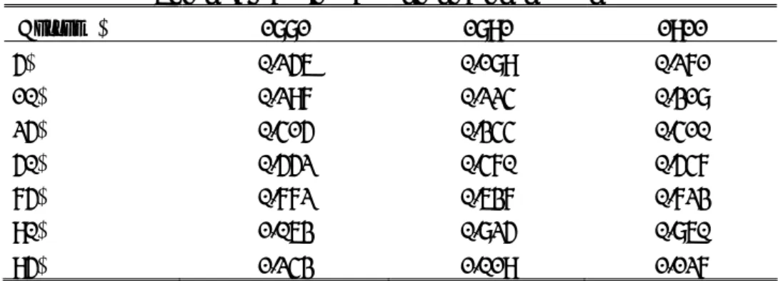
Table 2: Distribution of credit development Bottom % 1881 1891 1911 5% 0.256 0.189 0.271 10% 0.297 0.224 0.318 25% 0.415 0.344 0.410 50% 0.552 0.470 0.547 75% 0.772 0.637 0.723 90% 1.063 0.825 0.860 95% 1.243 1.019 1.127
Interpretation: In 1882, credit development in the median département is equal to 0.552.
Map 1: Variation in credit development from 1881 to 1911 Pale yellow when >0.1; yellow between 0.1 & 0; orange between 0 & -0.1;
red when < -0.1. Paris and its suburbs are excluded from the map
Interpretation: in a given département, if credit/GDP is 0.6 in 1882 and 0.4 in 1910, the variation in credit development is 0.4-0.6=-0.2<-0.1, hence, the colour is red.
Also, the basic statistics point up some facts. First, standard deviations of credit development are 0.39 in 1881, 0.32 in 1891 and 0.30 in 1911 while median and mean values are respectively 0.55, 0.47 and 0.55 and 0.64, 0.54 and 0.60. These results suggest a catching up effect. This is also confirmed by the growth in the 10th percentile figure and the decrease in the 90th percentile figure (Table 1). The growth also seems to benefit the
northern developing départements rather than the more depressed south-western ones16 (See Map 1). Moreover, credit development is lower across all the départements in 1891, irrespective of wealth and development.
IV. Empirical tests
a. Econometric specifica ion t
Panel data is the strongest econometric tool for our research in its assessment of the effect of the Banque branch network in space and time. Since we are interested in the effect of geographical access to the Banque branches, we test the correlation between Banque branch density and credit development. We add some control variables and time and regional fixed effects to prevent missing variable bias. So the model we test is:
i t it k t i k k t i t i SUC CONTROL K u u CREDEV, =α. , +
∑
β ,, + + + +ε , (3)where CREDEV is credit development, SUC is either Banque branch density or the number of Banque branches, CONTROL is the set of control variables, K is a constant, u is a dummy, ε is the error term, i is the département index and t the time index, and k is the control variable index. The départements of “Seine” and “Seine et Oise” are excluded from our regressions (see discussion below).
Credit development is captured by two ratios. The first (traditional) ratio is the amount of credit to GDP. This ratio depends therefore on the quality of our GDP data. A comparison with Toutain’s recent calculations (see Combes et al. 2008) for 1862 and 1896 proves the accuracy of our device. Nevertheless, we want to dissipate any doubt by using another ratio. So we test credit development by the amount of credit per firm. This ratio is imperfect. Indeed, a large number of firms is not a corollary of wealth. The first ratio tests are therefore the best, whereas the second ratio tests confirm the direction of the results.
Banque branch density is merely the number of Banque branches per hectare for each area. This ratio easily captures average distance to the Banque. Note that the Banque branches include branches. Banque sub-branches depended on the nearest Banque branch, but practised the rediscounting of bills as well. Gonjo (2003) shows that sub-branches played the same role even though they were not directly controlled by a Banque de France inspector.
Control variables are the number of firms per capita, average firm size, population density and the number of bank branches per capita. Firms
16 Note that phylloxera hit wine productivity hard in the south-west of France.
are evaluated using business tax statistics. This tax is paid by all firms in all lines of business save agriculture. Average firm size is defined as non-agricultural production divided by the number of firms.
The number of firms per capita17, population density and average firm size take into account the impact of market size. As summed up by Levine (2005), the larger the economy, the greater the financial development. Furthermore, as proved by Petersen and Rajan (1997) and Biais and Gaulier (1997), the trade credit supply increases with wealth and average firm size. However, firms tend to finance themselves as their size increases.
There are two different reasons for using bank branches per capita. First, the banking population is very important in the determination of credit development. Second, if the Banque chose to set up branches for pure profit reasons, this variable would rub out the Banque branches effect.
Départements and time fixed effects control for local trends, as mentioned in the presentation of the credit development data. They also help to take into account local institutions. All in all, they are a traditional way of producing robust estimates.
The INED website (www.ined.fr) provides the population figures per French département. Jobert (1991) supplies the business tax statistics. The Bottin du Commerce et de l’Industrie is used to evaluate the number of bank branches.
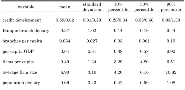
Table 3: Statistics summary
variable mean deviation standard percentile 10% percentile 50% percentile 90%
credit development 0.59/0.82 0.31/0.73 0.28/0.34 0.55/0.66 0.93/1.33
Banque branch density 0.37 1.02 0.14 0.19 0.44
branches per capita 0.064 0.027 0.03 0.061 0.10
per capita GDP 0.64 0.31 0.38 0.58 0.92
firms per capita 0.49 1.24 3.29 4.80 6.51
average firm size 6.90 3.19 4.20 6.16 10.82
population density 0.69 0.43 0.42 0.59 1.08
Interpretation: on average there is 6F of credit per 10F of production or 820F per firm, 3.7 Banque branches per 10,000 Ha, 6.4 bank branches per 10,000 inhabitants, production of 6,400F per capita, 4.8 firms per 100 inhabitants, 7F in business tax per firm, 327 inhabitants per Ha. “Seine” is excluded.
17 This variable is excluded when the dependant variable is calculated using the number of firms as denominator.
b. Results
Table 4 displays within regressions with time dummies18. Our results highlight two points of interest. First, though the Banque branch effect is positive, it is small and weak. Second, the result holds only for the first calculation of credit development.
Table 4
Determinant of credit development
The dependant variable is credit/GDP in [1] and [2] and credit/firms in [3] and [4]. All the regressions add time and geographic fixed effects.
Independent
variables [1] [2] [3] [4]
Banque branch density 0.22* 0.27
(0.12) (0.20)
number of Banque branches 0.04** 0.05
(0.18) (0.03)
population density -0.56** -0.57** -0.70** -0.70**
(0.25) (0.25) (0.34) (0.33)
firms per capita -0.11 -0.07
(0.36) (0.34)
average firm size -0.11 -0.10 0.47** 0.47**
(0.20) (0.19) (0.22) (0.21)
bank branches per capita 0.15** 0.15** 0.14* 0.14*
(0.06) (0.06) (0.08) (0.08) constant 0.92*** 0.91*** 0.73*** 0.72*** (0.34) (0.32) (0.10) (0.10) R² within 0.23 0.24 0.26 0.26 N 248 248 248 248
***, ** and * significant at 1%, 5% and 10%. Robust standard errors in brackets.
Interpretation: As there is on average one Banque branch per 160,000 Ha, one Banque branch accounts for 0.22*0.16=0.035 of the first credit development ratio. One bank branch also accounts for (0.15)*(0.026)=0.004.
A Banque branch accounts on average for 0.035 points of credit development. In the median département whose credit development indicators are 0.55 and 0.66, a Banque branch accounts for 6.4% of this
18 We only report results with fixed effects since the Hausman test proves the inconsistency of random ones.
value. This effect becomes 7.5% in [2], 7% in [3] and 7.5% in [4]19. The standard errors suggest that [2] is the most accurate coefficient.
However, there is some risk of bias. There is evidence that the Banque set up new Banque branches in industrial areas where it could make profits. Therefore, even if we introduce control variables to eradicate this effect, some problems could remain.
The Banque branch committee meeting minutes contain evidence of both profit seeking and public interest motives. Each branch authorisation entailed a detailed cost-benefit analysis by the Banque and city businessmen. The Banque always sought to balance both interests. Nevertheless, as long as the Banque was sure to make profits, it was an open-and-shut case. For instance, the report on the Bethume sub-branch said, “This city has incomparable wealth and industrial and commercial business.” While some branches were set up by public interest operations, many others were in the Banque’s own interest. Nonetheless, three points should be added. First, even if the Banque decided to set up branches based solely on profit criteria, no branches were opened without prior authorisation. Second, the Banque never chose to set up a new Banque branch alone. It had to apply to the city first and required government authorisation. Third, the archives only give the official story. There is thus no evidence of the wishes of the ‘governor’, as many decisions were made unofficially by powerful politicians.
Lastly, there is the issue of omitted variables. The Banque branch variable can thus be correlated with unobserved effects such as phylloxera and industrial shocks. Phylloxera, for instance, could strongly reduce the estimated coefficient of our OLS regressions. In general, many elements could positively or negatively influence the estimated effect of the Banque branches on credit development.
V. Instrumental variables and robustness
a. Instrumental variables: presentation and results
We have identified a basic problem with the previous OLS result: the Banque de France was a private institution! It set up new branches if the expected profits were sufficient. Expected profits could, however, be correlated with credit development. Also, in this respect, the sum of economic components entering into the Banque’s decision bears the risk of missing variables. We have therefore chosen to use instrumentation.
Given the political influence exerted on the Banque, the share of the population of the first and second city (five years before the observation of
19 [3] and [4] assess the effect of Banque branches on the second indicator of credit development.
credit development) is a nice instrument20. This choice is motivated by two arguments. First, with the renewal of the monopoly of issue in 1897, the Banque was legally obligated to set up a Banque branch in all French “Prefectures”. Though the “prefecture” is often a main town, it is not necessarily the biggest city in the département21. The relative size of the second city is thus positively correlated with the number of Banque branches in the area. Second, the mayor of a large city in the area had strong political influence. So if the size of the second city is close to the size of the first city, lobbies should pressurise the government to set up a Banque branch, especially when the two cities are not too near to one another. On other hand, if the first city is predominant,22 there is less incentive to set up an additional Banque branch even though the second city is large23. Archives provide many examples of political pressure from cities. In all cases, “départemental” city influence is predominant. Indeed, the electoral map shows that the mayor of a locally influential city gained easy access to the top of the administration.
Evaluation of the effect of both IVs upon the number of Banque branches is as expected. The share of the first city has a strong negative effect. If this share increases by 10%, the number of Banque branches is reduced by one unit. At the same time, the share of the second city has a positive effect. If it increases by 5%, the number of Banque branches increases by one unit.
Although the EI-test24 (exogeneity of instruments) and J-test of our regressions confirm the quality of our instrumentation, a large second city could be said to be a consequence of wealth (even if fixed effects and population density are still used). Also, the size of the first city is directly correlated with commercial development. We thus create another IV. We merely use the difference between the share of the first and the second city. As a result, rural areas can get a high IV figure even though the first and
é t
20 It is worth noting that the size of the two cities is not statistically correlated. 21
22 départements were in this case in 1896, which corresponds to 27% of all the départements in our panel. To demonstrate the importance of this fact, we built a variable equal to 1 if the prefecture is not the biggest city in the d par ement and 0 otherwise. The corresponding dummy variable is significant (p=0.06) and positively linked (a=0.34) to the number of Banque branches in 1911. Here, control variables are those previously used plus per capita GDP plus the share of population of the first and the second city plus the urban population (R²=0.85). If we withdraw the share of population of the second city from the set of control variables, the effect increases (0.44) and is highly significant (p=0.01) (R²=0.84). This outcome suggests that both variables exert a similar effect. Full regressions are available on request from the author.
22 This means that the second city’s population share is small even if it has a large population.
23 The example of the département in which Lyons is situated bears out this hypothesis. 24
We also check for Stock & Yogo statistics to confirm the instrumentation. Results prove that the instruments are not weak, especially in the second IV set. Results are available on request from the author.
second cities are small. Nonetheless, we unfortunately lose the ability to test the entire accuracy of the instrumentation with the J-test25.
Again, the results point to the same conclusions. On average, if the difference in the share of both cities decreases by 7%, the number of Banque branches increases by one unit.
Of course, IVs do not take into account cases with more than two Banque branches. However, in such situations, the areas should have a large second city anyway.
Table 5: Determinants of credit development using IV-GMM
The dependant variable is credit/GDP in [1] and [2] and credit/firms in [3] and [4] GMM-IV regressions with time and geographic fixed effects. The IVs are the population share in the first and second city.
Independent
variables [1] [2] [3] [4]
Banque branch density 0.84** 0.94**
(0.34) (0.37)
number of Banque branches 0.13*** 0.14**
(0.05) (0.06)
population density -0.11*** -0.10*** -0.13*** -0.11***
(0.04) (0.04) (0.05) (0.04)
firms per capita -0.49 -0.31
(0.39) (0.34)
average firm size -0.20 -0.17 -0.38* -0.41**
(0.22) (0.19) (0.22) (0.20)
bank branches per capita 0.13** 0.13** 0.10 0.11 (0.05) (0.05) (0.07) (0.07) constant 0.37*** 0.41*** 0.40*** 0.37*** (0.11) (0.11) (0.12) (0.10) N 248 248 248 248 J-Test 0.65 0.63 0.62 0.62 EI-Test 0.009 0.006 0.019 0.010 WH-Test 0.027 0.028 0.069 0.087
***, ** and * significant at 1%, 5% and 10%. Robust standard errors in brackets
25 The J-test is a test of over-identification. It is calculated if, and only if, the number of instruments is greater than the number of instrumented variables.
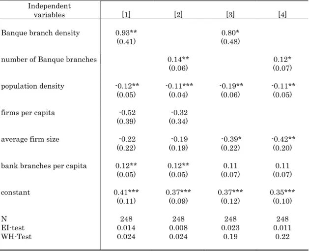
Table 6: determinants of credit development using IV-GMM
The dependant variable is credit/GDP in [1] and [2] and credit/firms in [3] and [4] GMM-IV regressions with time and geographic fixed effects. The IV is the difference in population share between the first and second city.
Independent
variables [1] [2] [3] [4]
Banque branch density 0.93** 0.80*
(0.41) (0.48)
number of Banque branches 0.14** 0.12*
(0.06) (0.07)
population density -0.12** -0.11*** -0.19** -0.11**
(0.05) (0.04) (0.06) (0.05)
firms per capita -0.52 -0.32
(0.39) (0.34)
average firm size -0.22 -0.19 -0.39* -0.42**
(0.22) (0.19) (0.22) (0.20)
bank branches per capita 0.12** 0.12** 0.11 0.11 (0.05) (0.05) (0.07) (0.07) constant 0.41*** 0.37*** 0.37*** 0.35*** (0.11) (0.09) (0.12) (0.10) N 248 248 248 248 EI-test 0.014 0.008 0.023 0.011 WH-Test 0.024 0.024 0.19 0.22
***, ** and * significant at 1%, 5% and 10%. Robust standard errors in brackets.
We use a GMM estimator26. In the first set of the IV estimation, we systematically test for instrument quality using the EI-test and the J-Test. In each case, the instruments are validated. We also run a Wu-Hausman test to assess the endogenous bias; results give evidence of its existence. The IV results are displayed in Table 5 and Table 6.
A Banque branch accounts in the first set of IV regressions for 0.13/0.14 points of credit development, which corresponds to 25%/22% of the median level. As there are two Banque branches per area on average, a département without Banque branches would see a 52%/46% reduction in its credit development. The EI tests prove that the instruments are not
26 The GMM estimator may be weak if the sample is too small. It tends indeed to reduce the p-value of the student test. We therefore test our model using the basic 2SLS regression. Since the p-values maintain very similar values, our GMM estimations are devoid of such bias.
weak, whereas the J-tests show they are not endogenous. Note the signs of the instruments are those we expected theoretically27.
The results are fairly similar in the second set of IV regressions. [1] increases by 0.10 points while [2] presents the same results as in the first IV set. [3] and [4] present weaker coefficients with lower confidence levels. The effect dwindles to 0.12 points, which corresponds to 18% of the median level.
By comparison with previous OLS results, the effect is on average multiplied by four. Also, the coefficient determined by the IV regression appears to be more suitable given the Bank discount amounts involved. This indeed represents 21% of GDP in the average area in 1910. When normalised by the number of Banque branches, this figure becomes 15%. Therefore, the IV coefficients find that 1F discounted by a Banque branch generates 1.73F of credit on average while this amount is 0.41F in the basic OLS case. Also, unlike the OLS outcomes, the IV outcome provides evidence of a credit multiplication effect.
b. Robustness check
We check for robustness by adding the Banque branches’ profit into the regressions. The results remain the same, while the additional variable is insignificant. Given the nature of the identification bias, these results provide additional evidence of the suitability of our instrumentation. We also add at the same time the share of the urban population to get a better control of commercial development. Again, the results remain the same while the additional variable is insignificant (regressions on request from the author).
Instead of the previous IV, we use the information on the law of 1897 and the relative size of the prefecture in each département. Since 22 prefectures were not the biggest cities of their département in 1896, the number of Banque branches must be positively related (after 1897), with a dummy equal to 1 when the prefecture is not the biggest city of the département and 0 otherwise. According to the shape of the panel, the new IV is the multiplication of this dummy with the 1911 year dummy. Results are still positive even though the impact of Banque branches is weaker than above. The Banque branch accounts now for 12% of credit development. Significance is reduced as well. Estimations are significant at 10% with the first calculation of credit development, while they are near but above this threshold with the second calculation (p=0.11). Also, Stock & Yogo tests and EI-tests prove that the instrument respects the basic
27
In the first IV set, the coefficient of the population share of the first city is negative while the coefficient of the population share of the second city is positive. In the second IV set, the difference between both population shares is negative. All results are available on request from the author.
conditions of IV estimations, whereas the Hausman tests do not display endogenous bias anymore28. All in all, these estimations are logically less robust than those previously presented. Indeed, regarding the number of départements with an increase in Banque branches from 1897 to 1911, this IV matches with only one-third of all observations. In any case, these results confirm the previous ones and prove that our instrumentation strategy was good. The results are displayed in Table 9 in the appendix.
Lastly, we run cross-département regressions on temporal difference. The estimated variable becomes the difference in credit development from 1881 to 1911. We therefore test for the effect of the Banque branch variation (difference from 1881 to 1911), instrumented by the second IV in 1881 (difference between the share of the first and second city in 1881). We also add, aside from the usual control variables, figures representing how they differ over the period (we add in, for instance, the difference in population density from 1881 to 1911). The effect is strongly positive and highly significant. One additional Banque branch entails a positive variation of 0.09/0.11 points of credit development. Note that the EI-tests and WH-tests produce the same results as above. The results are displayed in Table 10 in the appendix29.
c. The “Seine” and “Seine et Oise” issue
An important fact has to be pointed up. All our regressions exclude the “Seine” and “Seine et Oise” areas30. Two reasons explain this choice. First, these départements are small with high populations. ‘Banque branch density’ is thus artificially high. Second, since the head office of the Banque is located in Paris, it attracts bills from others countries. This choice raises two questions. First, do head office particularities generate bias via the action of the largest companies located in Paris? For instance, did industrial firms in Le Creusot (Saône et Loire) discount their bills in Paris or in Macon? Second, did deposit banks discount their paper in Paris or at the nearest Banque branch?
‘Average firm size’ helps deal with the first issue. Its positive correlation with credit development dissipates any doubts about the large company bias. Furthermore, fixed effects capture these phenomena as long as they are stable over time.
Second, Lescure (2003) shows that Banque branches’ balance sheets were contained large volumes of deposit bank discounting. Some values are especially high in large cities (Lyons and Bordeaux). This fact is also
28 Even if endogenous bias is not proved empirically, the doubt remains theoretically. 29 Note that we only present the coefficients for the variable of interest. The other variables are available on request from the author. Nonetheless, there are no surprising outcomes. 30 Note that adding ‘Seine & Oise’ does not change the significance of results. However, the effect increases on average by 25%.
corroborated by Plessis (2001). Therefore, deposit bank branches discounted their bills at the nearest Banque branches.
VI. Discussion
What do these outcomes suggest about economic development? We know that credit development grows with the Banque branch network as long as the relationship remains a key point of the banking system. Nevertheless, did it bring about economic development? Subsequent authors could shed light on this issue. First, the system had no overall consistency and did not allow for any real monetary policies. In other words, the Banque acted in a microeconomic way instead of a macroeconomic way. Second, the system relies on a costly stock of gold and prevents the utilisation of modern monetary tools. Third, protection of small banks entailed a kind of economic ‘Jacobinism’. It thus prevented the emergence of large ‘universal’ banks more able to promote innovation and growth using modern credit tools, critics say.
Conversely, a number of arguments stress the positive effects of the Banque’s policy. First, Banque branches helped capital market integration especially in backward areas. Second, because of private information requests from the productive system, deposit banks could not find a counterpart to their short-term deposits in the modern and/or industrial sectors. Deposit banks thus chose to take over the safe business of trade credits. In response to this competition, local and regional banks took advantage of their private and local knowledge to move into in riskier, but highly productive businesses. In this respect, local and regional banks were closer to the German universal bank ‘ideal’ than deposit banks (see Lescure, 2009). Third, the Banque was flexible and often agreed to rediscount risky papers from industrial areas (see Nishimura, 1995). In this way, the Banque encouraged the use of modern credit tools basically needed by industry. Fourth, some market failings can appear. Although the deposit banks were highly profitable, their interests did not necessarily tie in with those of the markets driving growth.
VII. Conclusion
In an environment of poor access to money and strong credit constraints, the Banque de France became a central hub of the French financial system. This contribution shows that better access to the Banque branches improved bill liquidity and credit development.
The Banque relied on local bank positioning to implement its policy for a number of reasons. First, local banks were in the local business heartland. Second, these banks needed access to central liquidity. Third, the competition generated by the deposit banks led the Banque to change
its traditional activities. It was to cope with all these constraints that a large number of Banque branches opened after 1897. The outcome was considerable, as a Banque branch accounted for 26% of the credit development of the median geographic area.
Local bank monographs and the Banque archives show that the mechanism was simple. A Banque branch rediscounted a bank’s safe bills. The Bank was then encouraged to increase its credit to local firms to make profit. In turn, firms drafted more bills that were thus easily discountable to the bank. All in all, we evaluate that 1F discounted by a Banque branch triggered 1.73F of credit.
However, questions remain as to the effects of Banque policy on economic development. As mentioned above, previous studies on the topic (see Nishimura, 1995, and Moine, 2001) confirm the Banque’s positive impact on innovation and industrial investment at micro level. Nevertheless, by sustaining local activities, the Banque could prevent the appearance of large industries with a greater capacity to drive growth. The debate is of vital importance, but remains unsolved to date. Answers seem all the more imperfect as Banque policy was part of a complex and embedded institutional structure. In other words, the efficiency of Banque policy should be appraised in terms of its objectives. From this point of view, the present paper is quite optimistic.
Lastly, the results open up prospects for developing economics. This study concerns backward economies in small business areas with substantial local banking structures. It consequently highlights the government’s responsibility in addressing credit constraints and credit development. Given that many countries have similar banking structures today (see Russia for instance), this paper is not a “mere historical case”. References
Alessandrini, P., Presbitero, A., F., Zazzaro, A., “The effect of cross-border bank mergers on bank risk and value”, Università Politecnica delle Marche – Quaderni di discussion (266), 2006
Baubeau, P., Thèse de doctorat d'Université : Les « cathédrales de papier » ou la foi dans le crédit. Naissance et crise du système de l’escompte en France, fin XVIIIe-premier XXe siècles, under the direction of Michel
Lescure, at the University of Paris X Nanterre, 2004
Bazot, G., “Finance and growth: local banking, credit and innovation in XIXth France”, PSE-WP, 2010
Berger, A., N., DeYoung, R., “Technological progress and the geographic expansion of the banking industry”, Journal of Money, Credit and Banking, Vol. 36, No. 6, 2006
Biais B., Gollier C., “Trade credit and credit rationing”, Review of financial studies, Vol.10, 1997.
Bouvier, J., “L’extension des réseaux de la monnaie et de l’épargne” in Braudel, F. & Labrousse E. Histoire économique et sociale de la France, Tom 3, Vol. 2, pp 391-429, PUF, 1979
Clapham, J., H., “Bank of England: A History 1694-1914”, 2 vol., Cambridge University Press, 1944
Combes, P., Lafourcade, M., Thisse, J., Toutain, J., "The rise and fall of spatial inequalities in France: A long-run perspective", PSE Working Papers, 2008
Flandreau, M., « Les règles de la pratique : La Banque de France, le marché des métaux précieux, et la naissance de l’étalon-or, 1848-1876 », Annales : Histoire Sciences Sociales, Vol. 51, No. 4, pp 849-872, 1996
Gonjo, Y., « La Banque de France et la décentralisation du crédit (1880-1914) », in Feiertag, O. and Margairaz M., « Introduction des pratiques et politiques des banques d’émission en Europe (XVII-XXèmes siècles) », Paris, Albin Michel, 2003
Hoffman, P.T., Postel-Vinay, G., Rosenthal, J.L., « Des marches sans prix. Une économie politique du crédit à Paris 1660-1870 », Paris, Ed. EHESS, 2001
Jobert, P., « Les entreprises aux XIXe et XXe siècles », Paris, Presses de l'E.N.S., 1991
Lemarchand, Y., « La comptabilité en France : Essais Historiques », Garland Publishing, New York, 1996
Lescure M., « La formation d’un système de crédit en France et le rôle de la banque d’émission : approche comparée », in Feiertag, O. and Margairaz M., « Introduction des pratiques et politiques des banques d’émission en Europe (XVII-XXèmes siècles) », Paris, Albin Michel, 2003
Levine, R., “Finance and growth, theory and evidence”, in Aghion, P. Durlauf, S. N., Handbook of Economic Growth, 2005
27
Levy-Leboyer, M., « Le crédit et la monnaie: l’apprentissage du marché » in Braudel, F. & Labrousse E. Histoire économique et sociale de la France, Tom 3, Vol. 2, pp 391-429, PUF, 1979
Mitchener, K. J., Ohnuki, M., “Institutions, competition, and capital market integration in Japan”, Journal of Economic History, Vol. 69, No. 1, pp 138-171, 2009
Moine, J.M., « Banque locale et financement de l’industrialisation : la banque Thomas et la sidérurgie du bassin de Longwy, 1863-1907 » in Lescure, M., Plessis, A., Banques locales et banques régionales en France au XIXe siècle, Albin Michel, 1999.
Nishimura, S., “The French provincial banks, the Banque de France, and Bill Finance, 1890-1913”, Economic History Review, Vol. 48, No. 3, 1995 Petersen, M. A., Rajan, R. G., "Trade Credit: Theories and Evidence," Review of Financial Studies, Oxford University Press for Society for Financial Studies, Vol. 10(3), pp 661-91 1997
Petersen, M. A., Rajan, R. G., “Does distance still matter? The information revolution in small business lending”, Journal of Finance,Vol. 57, 2002 Plessis, A., « La révolution de l’escompte dans la France du XIXe siècle », Revue d’Histoire du XIXe Siècle, No. 23, 2001
Rouleau, G., « Les règlements par effets de commerce en France et l’étranger », Paris, Société statistique de Paris, 1914
Stein J. C., “Information production and capital allocation: decentralised vs. hierarchical firms”, Journal of Finance, Vol. 57, 2002
Appendix 1: Credit development map
Credit development in 1881, 1891 and 1911
Appendix 2: GDP calculation by French département in 1881, 1892 and 1911
Our estimation uses Toutain’s series on agricultural production and the amount of business tax31. Given that business tax is levied on all trade and industrial sectors, it can be a good alternative to the actual calculation of non-agricultural output. Since the tax was also more or less proportional to the wealth of the firms, it turns out to be the perfect complement.
The proportional part of business tax was calculated on the basis of the rental value of all the productive inputs. If a firm had more than one business located in different areas, it had to pay the tax in each area proportional to the corresponding rental value. Rental value is, however, quite an opaque expression. In actual fact, the tax office determined the rental value of an establishment based on its expected level of production despite the potential existence of some intra- and inter-district disparities. We know, for instance, that the tax rate differed from one area to the next. We also know that inflation drove up rental values in some areas. We therefore have to assume that the combination of these effects is weak32. Although this single hypothesis is quite strong, a combination of small (ad hoc) hypotheses is often stronger at the end of the day. Moreover, it is unfortunately impossible to calculate historical series with complete accuracy. Evidence of this is found in the differences in the GDP series produced by Toutain and Levy-Leboyer33.
We therefore assume a constant coefficient from the business tax on non-agricultural production. This helps find the coefficient (β) relating to the amount of tax on commercial and industrial value-added.
For each département, GDP is:
(1) Yi,t = Ai,t +βi,tPi,t
where Y is GDP, A is the production of the agricultural sector and P is the amount of tax, i is the département index and t the time index. For France as a whole, (1) is rewritten:
(1’)
∑
=∑
(
+)
i t i t i t i i t i A P Y, , β, ,Since we letβi =β, we obtain:
31
French tax of “la patente”.
32 Note that one bias can often offset another.
t t t
t A P
Y = +β
Then we can determine the value of the coefficient: (2) t t t t P A Y − = β
As we know Y, A and P for all départements, it is easy to estimate GDP for each of them. We just have to put (2) in (1), then the equation is:
t i t t t t i t i P P A Y A Y, , , − + =
Utilisation of this equation provides GDP for all the départements. Of course, this calculation is an evaluation. Hence, some exogenous shocks on production could be erased by the estimation.
Given that no information is available on agricultural production per area for 1881, we estimate the data using the 1891 values. The calculation assumes a smooth spread of agricultural value-added from 1881 to 1891. This hypothesis is not heroic since factors of evolution are rather exogenous in the short run. The phylloxera that reached their peak during the period could, however, be a bias. Determination of GDP for 1881 is thus:
(3) ,1881 ,1891 ,1891 1881 1881 i,1881 i i i i A A A P Y ⎟ +β ⎠ ⎞ ⎜ ⎝ ⎛ =
∑
30Appendix 3: Tables
Table 7: Determinants of the growth in local bank branch density from 1881 to 1911
The dependant variable is the variation in the number of local and regional bank branches from 1881 to 1911. The panel includes all cities of more than 100,000 inhabitants plus cities with a “prefecture” or a “sub-prefecture”. [1] includes all cities covered by the data, [2] includes cities with less than 100,000 inhabitants in 1910 and [3] includes cities with less than 75,000 inhabitants in 1910. Population in thousands of inhabitants.
Independent
variables [1] [2] [3]
Variation in deposit bank branches per
inhabitant -0.46** -0.47** -0.48**
(0.22) (-0.23) (-0.23)
Population variation -0.21 -0.20 -0.16
(0.33) (0.13) (0.17)
Variation in Banque branches -0.16 -0.11 -0.09
(0.28) (0.27) (0.27)
Constant -0.01 -0.01 -0.01
(0.01) (0.03) (0.03)
R² 0.10 0.10 0.10
N 389 375 365
***, ** and * significant at 1%, 5% and 10%
Interpretation: an one-point increase in the density of deposit bank branches reduces local bank density by 0.46, 0.47 and 0.48 points in the given sample.
Table 8: Determinants of Banque profits by département
The dependant variable is the Banque’s profit for 1881, 1891, 1901 and 1911. Deposit bank market share is the number of deposit bank branches divided by the total number of branches in a département. Profits in thousands of francs; population in thousands of inhabitants; firms per hundred.
Independent
variables [1] [2]
deposit bank market share -0.21* -0.46***
(0.12) (0.13)
average firm size 0.56* 0.10
(0.28) (0.19)
Banque loans to GDP 0.63*** 0.69***
(0.10) (0.12)
number of Banque branches 0.06** 0.08**
(0.03) (0.03)
firms per capita 0.32 0.50**
(0.57) (0.21)
bank branches per capita 0.53 1.18**
(0.62) (0.51) per capita GDP 0.66 0.93*** (0.46) (0.30) population density 0.87 1.11 (1.72) (0.87) constant -1.16* -0.37*** (0.66) (.11)
individual effects fixe random
Hausman test p =0.0013
R² 0.64 0.73
N 336 336
***, ** and * significant at 1%, 5% and 10%, standard errors in brackets
Interpretation: a 1% increase in deposit bank market share reduces the Banque’s profits by 2,100 F.
Table 9: Determinants of credit development with IV-GMM
The dependant variable is credit/GDP in [1] and [2] and credit/firms in [3] and [4]. GMM-IV regressions with time and geographic fixed effects. The GMM-IV is the dummy for 1911 multiplied by the dummy “prefecture”, equal to one if the prefecture is not the biggest city in the département in 1881 and zero otherwise.
[1] [2] [3] [4]
Banque branch density 0.41* 0.59
(0.23) (0.38)
Banque branches 0.61* 0.85
(0.34) (0.54)
population density -0.71** -0.65** -1.00** -0.90**
(0.30) (0.25) (0.49) (0.41)
firms per capita -0.21 -0.11
(0.31) (0.29)
average firm size -0.13 -0.11 0.42** 0.45**
(0.17) (0.16) (0.19) (0.17)
bank branches per capita 0.15*** 0.15*** 0.12* 0.12*
(0.44) (0.44) (0.07) (0.07) Constant 0.28*** 0.27*** 0.34*** 0.32*** (0.08) (0.07) (0.11) (0.10) Observations 248 248 248 248 EI-test 0.001 0.001 0.004 0.001 WH-test 0.26 0.38 0.34 0.45
***, ** and * significant at 1%, 5% and 10%, standard errors in brackets