Air Quality, Infant Mortality, and the Clean Air Act of 1970
by
04-006 August 2003
Kenneth Y. Chay and Michael Greenstone WP
Air Quality, Infant Mortality, and the Clean Air Act of 1970*
Kenneth Y. Chay and Michael Greenstone
August 2003
* We thank David Card, Doug Almond, Josh Angrist, Gary Becker, David Cutler, John DiNardo, Carlos Dobkin, Mark Duggan, Vernon Henderson, Charles Kolstad, Jeff Milyo, Steve Pischke, and numerous seminar participants for helpful comments. Justin McCrary, Doug Almond, Fu-Wing Lau, and Anand Dash provided outstanding research assistance. Funding from NSF Grant No. SBR-9730212 and NIH (NICHD) Grants No. R01 HD42176-01 and R03 HD38302-01 is gratefully acknowledged.
Air Quality, Infant Mortality, and the Clean Air Act of 1970
AbstractWe examine the effects of total suspended particulates (TSPs) air pollution on infant health using the air quality improvements induced by the 1970 Clean Air Act Amendments (CAAA). This legislation imposed strict regulations on industrial polluters in “nonattainment” counties with TSPs concentrations exceeding the federal ceiling. We use nonattainment status as an instrumental variable for TSPs changes to estimate their impact on infant mortality changes in the first year that the 1970 CAAA was in force.
TSPs nonattainment status is associated with sharp reductions in both TSPs pollution and infant mortality from 1971 to 1972. The greater reductions in nonattainment counties near the federal ceiling relative to the “attainment” counties narrowly below the ceiling suggest that the regulations are the cause. We estimate that a one percent decline in TSPs results in a 0.5 percent decline in the infant mortality rate. Most of these effects are driven by a reduction in deaths occurring within one month of birth, suggesting that fetal exposure is a potential biological pathway. The results imply that roughly 1,300 fewer infants died in 1972 than would have in the absence of the Clean Air Act.
Kenneth Y. Chay Michael Greenstone
Department of Economics Department of Economics
University of California, Berkeley MIT
549 Evans Hall E52
Berkeley, CA 94720 50 Memorial Drive
and NBER Cambridge, MA 02142-1347
kenchay@econ.berkeley.edu American Bar Foundation and NBER mgreenst@mit.edu
Introduction
The 1970 passage of the Clean Air Act Amendments (CAAA) and the establishment of the
Environmental Protection Agency (EPA) marked an unprecedented attempt by the U.S. government to
mandate lower levels of air pollution. The stated goal of these efforts was to achieve air quality standards
that “protect the public health.” In the case of total suspended particulates (TSPs), widely thought to be
the most pernicious form of air pollution, the EPA set maximum allowable concentrations that every
county was required to meet.1 This study uses the reductions in TSPs concentrations induced by the 1970
CAAA to estimate the effects of TSPs on infant mortality.
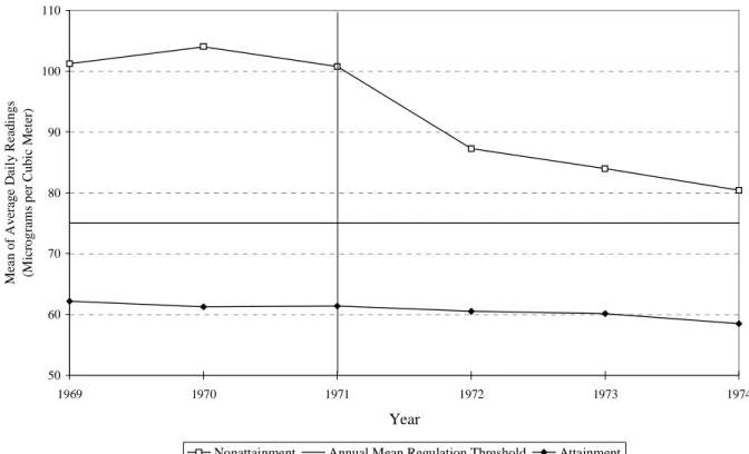
Figure 1 shows trends in average TSPs pollution and infant mortality rates for the entire United
States from 1970-1990.2 It is apparent that air quality improved dramatically in the 1970s and 1980s,
with particulate concentrations falling from an average of 95 micrograms-per-cubic meter (µg/m3) to about 60 µg/m3. Almost all of the reduction occurred in two punctuated periods, 1971-1973 and 1980-1982. The figure also shows the large decline in the infant mortality rate over the entire period. Although
both TSPs pollution and infant mortality rates trended downward, their time-series correspondence does
not provide conclusive evidence of a causal relationship. First, the punctuated declines in TSPs are not
mirrored in the infant mortality rate series. Further, other potential determinants of infant mortality (e.g.,
social insurance programs, medical technology) were also changing during this period.
Chay and Greenstone (2003) establish that most of the 1980-82 decline in TSPs was attributable
to the differential impacts of the 1981-82 recession across counties. The study uses the substantial
differences in air pollution reductions across sites to estimate the impact of TSPs on infant mortality. We
find that a one percent reduction in TSPs results in a 0.35 percent decline in the infant mortality rate at the
county level. Most of these effects are driven by a decline in deaths occurring within one month of birth,
1
In this period, the EPA defined TSPs to include all particles with diameters less than or equal to 100 micrometers (µm). The focus of federal regulation shifted to particulates with diameters less than or equal to 10 µm (PM10) and 2.5 µm (PM2.5) in 1987 and 1997, respectively.
2
The TSPs pollution series is based on averages across the 1,000-1,300 counties a year with TSPs monitors, while infant mortality rates are derived from the entire U.S. and are for all causes of death. The counties with TSPs data account for upwards of 80% of the U.S. population. Unless otherwise noted, infant mortality refers to death within the first year after birth.
suggesting that fetal exposure during pregnancy is a potential pathophysiologic mechanism. Overall, the
estimates imply that about 2,500 fewer infants died from 1980-82 than would have in the absence of the
dramatic reductions in particulates pollution.
In view of the significance of a potential causal link between TSPs pollution and infant mortality,
we believe it is important to validate the results from our analysis of the early 1980s. In this paper, we
examine data on infant mortality and air pollution from the other major episode of substantial changes in
TSPs levels in the early 1970s. We begin by demonstrating that these changes are largely attributable to
the 1970 CAAA. This legislation divided all U.S. counties into TSPs nonattainment and attainment
categories based on whether their ambient TSPs concentrations were above or below the legislated
maximum. Industrial emitters of TSPs were subject to significantly stricter regulations in nonattainment
counties than in attainment ones. We find that the entire decline in TSPs during the early 1970s occurred
in nonattainment counties and that two-thirds of the 1971-1974 decline in these counties occurred
between 1971 and 1972, the first year that the 1970 CAAA was in force. Consequently, this study uses
nonattainment status as an instrumental variable for 1971-1972 changes in TSPs to estimate their impact
on changes in infant mortality.
This research design has several attractive features. First, it is plausible that federally-mandated
regulatory pressure is orthogonal to county-level changes in infant mortality rates, except through its
impact on air pollution – thus, nonattainment status may be a valid instrument. Second, nonattainment
status is a discrete function of the previous year’s TSPs levels. This discontinuity in the assignment of
regulations can be used to gauge the credibility of the research design. Third, our analysis provides direct
and easily interpreted estimates of the air quality and health benefits of the 1970 Act – benefits that can be
compared with the costs to industry of complying with the regulations.
Finally, this study provides a unique opportunity to cross-validate the results from our earlier
work by examining a different design applied to a different era. In contrast to the recession-driven TSPs
reductions of the early 1980s, we use regulation-induced changes that occurred during an economic
expansion (1971-1972). Thus, any potential biases due to economic shocks are likely to be mitigated.
result, we can examine a different range of the pollution-infant mortality function and analyze the health
benefits at the federally mandated concentration ceiling.
We implement the design using the most detailed and comprehensive data available on infant
births, deaths, and TSPs levels for the 1969-1974 period. We find that the federally imposed county-level
regulations are associated with large reductions in both the TSPs pollution levels and infant mortality
rates of nonattainment counties. We estimate that a one percent reduction in TSPs results in a 0.5 percent
decline in the infant mortality rate at the county level. As in our earlier study, most of these effects are
driven by a reduction in the number of deaths occurring within one month of birth, suggesting that fetal
exposure is a potential biological pathway.
Our attempts to probe the robustness of these conclusions suggest that the instrumental variables
estimates of the effect of TSPs pollution on infant mortality are far less sensitive to specification than
conventional cross-sectional and fixed effects estimates. Further, the timing and location of the TSPs and
infant mortality improvements correspond remarkably well. As a test of internal validity, we find that the
regulation-induced TSPs reductions are uncorrelated with infant deaths due to accidents and homicides.
Finally, nonattainment and attainment counties near the federal ceiling exhibit discrete differences in
TSPs and infant mortality changes, but do not exhibit differences in other observable characteristics. This
provides our most convincing evidence that the regulations are causally related to declines in both TSPs
and infant death.
Overall, our findings support the conclusions that air pollution has a causal effect on infant
mortality and that the 1970 CAAA provided significant health benefits by reducing TSPs concentrations.
The estimates imply that roughly 1,300 fewer infants died in 1972 than would have in the absence of the
Clean Air Act. Also, the results correspond well with the findings in Chay and Greenstone (2003).
The paper proceeds as follows. Section I provides background on the 1970 Clean Air Act.
Sections II and III discuss the research design and the econometric methods used to implement this
design. Section IV summarizes the data, and Section V presents the empirical findings. Section VI
I. Background on the 1970 Clean Air Act Amendments
Before 1970 the federal government did not play a significant role in the regulation of air
pollution, a responsibility left primarily to state governments.3 In the absence of federal legislation, few
states acted to impose strict regulations on polluters within their jurisdictions. Concerned with the
detrimental health effects of persistently high concentrations of suspended particulates pollution, and of
other air pollutants, Congress passed the Clean Air Act Amendments of 1970.
The centerpiece of the 1970 CAAA was the establishment of separate federal standards, known as
the National Ambient Air Quality Standards (NAAQS), for six pollutants. The CAAA’s goal was to
reduce local air pollution concentrations so that all U.S. counties would be in compliance with the
NAAQS by 1975 (with the possibility of an extension to 1977). The first step in this process was the
assignment of pollution-specific “attainment-nonattainment” designations to all U.S. counties for each of
the regulated pollutants.4 For TSPs pollution the EPA was required to designate a county as
nonattainment if its TSPs concentrations exceeded either of two thresholds: 1) the annual geometric mean
concentration exceeded 75 µg/m3, or 2) the second highest daily concentration exceeded 260 µg/m3. This standard prevailed from 1971 until 1987, when the EPA shifted its focus to the regulation of finer
particles.
To achieve these standards, the fifty states were required to formulate and enforce State
Implementation Plans (SIPs) that specified precise abatement activities. For nonattainment counties, the
SIPs detailed plant-specific regulations for every major source of pollution. These local rules ordered that
any substantial investment by a new or existing plant must be accompanied by the installation of
state-of-the-art pollution abatement equipment and strict emissions ceilings. The SIPs also set emission limits for
existing plants in nonattainment counties.
3
Lave and Omenn (1981) and Liroff (1986) provide more details on the CAAAs. In addition, see Greenstone (2002) and Chay and Greenstone (2000).
4
It is unclear whether the EPA assigned nonattainment status at the county level or at a more aggregate geographic unit in the early 1970s. Our analysis assumes that the assignment was at the county level. The rationale for this choice is discussed in the “Nonattainment Data” subsection of the Data Appendix. Further, below we find that using nonattainment designations at a more aggregate geographic level does not change this paper’s qualitative findings.
In stark contrast to the oversight in nonattainment counties, the restrictions on industrial polluters
in attainment counties were considerably less stringent. Large-scale investments, such as new plants and
large expansions at existing plants, required the installation of less expensive (and less effective) pollution
abatement equipment. Moreover, existing plants and smaller investments were essentially unregulated.
Both the states and the federal EPA were given substantial enforcement powers to ensure that the
goals of the CAAA were met. To limit variation in the intensity of regulation across states, the federal
EPA had to approve all state regulation programs. On the compliance side, states initiated their own
inspection programs and frequently fined non-compliers. Further, the EPA was required to impose its
own procedures for attaining compliance in states that failed to adequately enforce the standards.
The 1970 CAAA was signed into law by Richard Nixon on December 31, 1970. Four months
later on April 30, 1971, the EPA announced the final publication of the NAAQS that specified the
national standards for TSPs concentrations. On August 14, 1971, the EPA published “Requirements for
Preparation, Adoption and Submittal of Implementations Plans” in the Code of Federal Regulations,
which set forth how states were to write their SIPs in order to achieve compliance with the NAAQS by
1975. Finally, the SIPs were due to the EPA by January of 1972, the first year in which the CAAA was
enforced. Appendix Table 1 shows the timeline of the key dates associated with the 1970 CAAA, and the
Data Appendix gives additional details.
Henderson (1996) provides evidence that the regulations were successfully enforced. He finds
that ozone concentrations declined more in counties that were nonattainment for ozone than in attainment
counties. Chay and Greenstone (2000) find that TSPs levels fell substantially more in counties that were
nonattainment for TSPs than in attainment counties after the passage of the 1970 CAAA and throughout
the 1970s.5
5
Greenstone (2002) provides further evidence on the effectiveness of the regulations. He finds that nonattainment status is associated with modest reductions in the employment, investment, and shipments of polluting
manufacturers. Interestingly, the regulation of TSPs has little association with changes in employment. Instead, the overall employment declines are driven mostly by the regulation of other air pollutants.
II. Research Design
Previous research has documented a statistical association between TSPs concentrations and adult
mortality.6 However, the reliability of the evidence has been seriously questioned for several reasons.
First, since air pollution is not randomly assigned across locations, previous cross-sectional studies may
not be adequately controlling for a number of potential confounding determinants of adult mortality (Pope
and Dockery 1996; Fumento 1997). For example, areas with higher pollution levels also tend to have
higher population densities, different economic conditions, and higher crime rates, all of which could
impact adult health. Second, the lifetime exposure of adults to air pollution is unknown. Many studies
implicitly assume that the current pollution concentration observed at a site accurately measures each
resident’s lifetime exposure. Third, the excess adult deaths that are attributed to temporarily elevated air
pollution levels in time-series studies may be occurring among the already sick and represent little loss in
life expectancy (Spix, et al. 1994; Lipfert and Wyzga 1995).
In the absence of randomized clinical trials, this study uses the air quality improvements induced
by the 1970 Clean Air Act Amendments in the first year that they were in force to estimate the impact of
TSPs on infant mortality. A research design based on comparisons between nonattainment and
attainment counties has several attractive features.7 First, TSPs nonattainment status is associated with
sharp differences in changes in TSPs across sites in the early 1970s. Panel A of Figure 2 shows the trends
in TSPs levels from 1969 to 1974 separately for counties that were nonattainment and attainment for
TSPs in 1972 – the first year of CAAA enforcement.8
6
Studies of the adult mortality effects of particulates pollution include Lave and Seskin (1977), Pope and Dockery (1996), Dockery and Pope (1996), Dockery, et al. (1993), and Pope, et al. (1995). Chay, Dobkin, and Greenstone (2003) examine the association between adult and elderly mortality and regulation-induced TSPs declines. 7
Despite extensive efforts, we were unable to obtain a list of the counties that were initially designated TSPs nonattainment by the EPA. Given the timeline for states to comply with the CAAA, states likely ascertained the identity of the counties with TSPs concentrations above the NAAQS while writing their SIPs during the second half of 1971. We assume that they relied on the available TSPs concentrations data from 1970 to determine which counties would be nonattainment for 1972. Thus, we assign counties with TSPs concentrations exceeding the NAAQS in 1970 to the 1972 TSPs nonattainment category. All other counties with nonmissing TSPs data are designated attainment for that year. The measures of TSPs concentrations are derived from the same network of TSPs monitors used by the states and the EPA in this period. The Data Appendix provides further details on our assignment rule.
8
The sample consists of the 401 counties with continuous monitor readings from 1969-1974 – 229 of these counties are TSPs nonattainment in 1972. Together these counties account for almost 60 percent of all births in the U.S. in
The figure documents that before the 1970 CAAA, TSPs concentrations were 40-µg/m3 higher in nonattainment counties. While the pollution trends are similar in the two groups from 1969 to 1971, there
is a sharp break in trend in nonattainment counties after implementation of the CAAA. From 1971-74
newly regulated counties had a stunning 20-µg/m3 reduction in TSPs, while TSPs fell by only 3 µg/m3 in attainment counties. These comparisons suggest that virtually the entire national decline in TSPs from
1971-74 in Figure 1 was attributable to the regulations. In addition, two-thirds of the 1971-74 TSPs
decline in nonattainment counties occurred from 1971-72, the first year of CAAA enforcement.
Consequently, our analysis focuses on this abrupt, one-year improvement in air quality.9
Second, below we find evidence that this design may reduce the role of omitted variables bias in
analyzing the association between TSPs and infant mortality. Panel B of Figure 2 displays the trends in
internal infant mortality rates (IMR) in the same two sets of counties.10 It shows that before the CAAA
was enforced, infant mortality rates were 120-150 deaths per 100,000 births higher in nonattainment
counties. Further, attainment and nonattainment counties had similar IMR trends between 1969 and
1971, with attainment counties experiencing a slightly larger decline. However, this pattern is reversed
between 1971 and 1972, with the attainment-nonattainment IMR gap narrowing by over 75 deaths per
100,000 births. The figure also reveals that attainment counties had a larger decline in infant mortality
between 1972 and 1974.
The correspondence of the trend breaks in TSPs and infant mortality differences between
nonattainment and attainment counties in 1972 suggests a causal relationship. Since the patterns after
1972 are less compelling, we probe the case for causality more rigorously in the analysis below. To
1970. 9
We probed how industrial polluters may have significantly reduced TSPs emissions in this narrow time frame. Electrostatic precipitators were one of the primary control devices used to abate particulates pollution during this period. The Industrial Gas Cleaning Institute reports that while annual sales of precipitators were approximately $50 million from 1968 through 1970, this figure doubled to $100 million in 1971 and 1972 (White 1984). According to Donald Hug of the Environmental Elements Corporation, a supplier of pollution abatement equipment, an
electrostatic precipitator ordered in 1971 could be operating in 1972. We conclude that the large decrease in TSPs emissions between 1971 and 1972 is the plausible result of polluter response to the 1970 CAAA.
10
We define internal infant mortality to be infant death due to health related causes (i.e., 8th International Classification of Diseases (ICD) codes 001 through 799). This excludes non-health related “external” causes of death such as accidents and homicides (i.e., 8th ICD codes 800 through 999).
maximize the signal-to-noise ratio in TSPs changes and minimize the potential biases from confounding
changes in other variables, we focus on the striking one-year changes that occurred between 1971 and
1972. The analysis uses nonattainment status as an instrumental variable for 1971-1972 changes in TSPs.
Since federally-mandated regulatory pressure is plausibly orthogonal to changes in infant mortality rates,
except through its impact on air pollution, nonattainment status may be a valid instrument. Consistent
with this, we find little association between nonattainment status and other observable variables,
including parents’ characteristics, prenatal care utilization, and transfer payments from social programs.
Further, nonattainment status in 1972 was a discrete function of the annual geometric mean and
second highest daily concentrations of TSPs in the regulation selection year, 1970. Thus, the assignment
of regulatory status has the feature of a quasi-experimental regression-discontinuity design (Cook and
Campbell 1979). If other factors affecting infant mortality are similar for counties just above and just
below the regulatory thresholds, then comparing outcome changes in nonattainment and attainment
counties with pre-regulation TSPs levels just around the threshold will control for all omitted factors
correlated with TSPs. Under this assumption discrete differences in mean outcome changes between
nonattainment and attainment counties near the federal ceilings can be attributed to the regulations. The
discontinuity in the assignment of regulations provides a valuable opportunity to gauge the credibility of
the research design and develop convincing specification tests.
Third, our focus on infant, rather than adult, mortality may circumvent the other important
criticisms of previous research. The problem of unknown lifetime exposure to pollution is significantly
mitigated, if not solved, by the low migration rates of pregnant women and infants. Thus, we assign TSPs
levels to infants based on the exposure of the mother during pregnancy and the exposure of the newborn
during the first few months after birth (we focus on deaths within 24 hours, 28 days, and 1 year of birth).
Further, since the mortality rate is higher in the first year of life than in the next 20 years
combined (NCHS 1993), it is likely that infant deaths represent a large loss in life expectancy. In
contrast, time-series studies of adult and elderly mortality based on daily air pollution fluctuations may be
detecting effects among the already very ill and dying. In this case, the actual loss of life expectancy may
A final advantage of the design is that it permits a direct analysis of the health benefits of TSPs
reductions at levels just above the EPA’s maximum allowable concentration. The optimality of the
CAAAs depends crucially on the existence and relative magnitudes of the health effects above and near
the federal regulatory threshold.
III. Econometric Methods
Our analysis compares changes in infant mortality rates and TSPs pollution from 1971-1972 for
counties that were nonattainment and attainment for TSPs in 1972. Here, we discuss the econometric
models used to estimate the infant mortality-TSPs association. For simplicity, it is assumed that the
“true” effect of exposure to particulates pollution is homogeneous across infants and over time.
The cross-sectional model predominantly used in the literature on air pollution and health is:
(1) yct = Xct′β + θTct + εct, εct = αc + uct
(2) Tct = Xct′Π + ηct, ηct = λc + vct,
where yct is the infant mortality rate in county c in year t, Xct is a vector of observed characteristics, Tct is
the mean of TSPs across all monitors in the county, and εct and ηct are the unobservable determinants of
infant mortality rates and TSPs levels, respectively. The coefficient θ is the “true” effect of TSPs on infant mortality. For consistent estimation, the least squares estimator of θ requires E[εctηct]=0. If there
are omitted permanent (αc and λc) or transitory (uct and vct) factors that covary with both TSPs and infant
mortality, then the cross-sectional estimator will be biased.
With repeated observations over time, a “fixed-effects” model implies that first-differencing the
data will absorb the permanent county effects, αc and λc. This leads to:
(3) yct - yct-1 = (Xct - Xct-1)′β + θ(Tct - Tct-1) + (uct - uct-1)
(4) Tct - Tct-1 = (Xct - Xct-1)′Π + (vct - vct-1).
For identification, the fixed effects estimator of θ requires E[(uct - uct-1)(vct – vct-1)]=0. That is, there are
no unobserved shocks to TSPs levels that covary with unobserved shocks to infant mortality rates.
While first-differencing removes permanent sources of bias, it may magnify any attenuation bias
a county, it imperfectly captures individual exposure to TSPs.11 This mismeasurement will attenuate the
estimated TSPs regression coefficient leading to a bias that is proportional to the fraction of the total
variation in TSPs that is attributable to measurement error. To the extent that the serial correlation in
“true” TSPs exposure is greater than the autocorrelation in the TSPs measurement error, first-differencing
the data will increase the magnitude of the attenuation bias.12
Now suppose there exists an instrumental variable, Zc, that causes changes in TSPs without
having a direct effect on infant mortality rate changes. Such a variable would purge the estimates of the
biases due to both omitted variables and measurement error. One plausible instrument is the 1970 CAAA
regulatory intervention for TSPs, measured by the 1972 attainment-nonattainment status of a county.
Here, equation (4) becomes:
(5) Tc72 - Tc71 = (Xc72 - Xc71)′ΠTX + Zc72ΠTZ + (vc72 - vc71), and
(6) Zc72 = 1(Tc70 > T ) = 1(vc70 > T - Xc70′Π - λc),
where Zc72 is the regulatory status of county c in 1972, 1(•) is an indicator function equal to one if the
enclosed statement is true, and T is the maximum concentration of TSPs allowed by the federal
regulations. Regulatory status in 1972 is a discrete function of 1970 pollution levels.13
An attractive feature of this research design is that the reduced-form relations between 1972 TSPs
nonattainment status and the two endogenous variables provide direct estimates of the benefits of the
regulations. In particular, ΠTZ from equation (5) measures the 1971-1972 air quality improvement in
nonattainment counties relative to the change in attainment counties. In the other reduced-form equation,
(7) yc72 - yc71 = (Xc72 - Xc71)′ΠyX + Zc72ΠyZ + (uc72 - uc71),
11
During the 1971-1972 period, the mean and median numbers of monitors in a county are 4.2 and 2, respectively. 12
However, in our context it is unclear whether the serial correlation in the TSPs measurement error from 1971 to 1972 is smaller or larger than the serial correlation in true TSPs exposure.
13
For simplicity, we have written (6) as if regulatory status is a function of a single threshold crossing. If Tcavg70 and max
70 c
T are the annual geometric mean and 2nd highest daily TSPs concentrations, respectively, then the actual regulatory instrument used is 1(Tcavg70 > 75 µg/m
3
or Tcmax70 > 260 µg/m
3
). Only six counties were nonattainment in 1972 for exceeding the 2nd highest daily concentration threshold, but not the annual geometric mean ceiling. See footnote 7 and the Data Appendix for details on the timing of the CAAA intervention.
ΠyZ captures the relative improvement in the infant mortality rate in nonattainment counties between 1971
and 1972.
Since the instrumental variables (IV) estimator (θIV) of the effect of TSPs on infant mortality is
exactly identified, it is equal to the ratio of the two reduced-form relations – i.e., θIV = ΠyZ/ΠTZ. Two
sufficient conditions for θIV to provide a consistent estimate of the TSPs effect are ΠTZ≠ 0 and E[vc70(uc72
- uc71)]=0. The first condition requires that the regulations induced air quality improvements. The second
condition requires that transitory shocks to TSPs levels in 1970 are orthogonal to unobserved shocks to
infant mortality rates from 1971-1972.14
Even if E[vc70(uc72 - uc71)] ≠ 0, causal inferences on θ may be possible by leveraging the
regression discontinuity (RD) design implicit in the 1(•) function that determines nonattainment status. For example, if E[vc70(uc72 - uc71)] = 0 in the neighborhood of the regulatory ceiling (i.e., 75 µg/m
3
), then a
comparison of changes in nonattainment and attainment counties in this neighborhood will control for all
omitted variables. Below, we present IV estimates based on all counties and RD estimates in which the
sample is limited to counties with TSPs concentrations “near” the 75 µg/m3 threshold in the regulation selection year.15 In the next section, we show that the observable characteristics of nonattainment and
attainment counties near the federal TSPs ceiling are very similar.
Another potential source of bias comes from unmeasured state-specific determinants of infant
mortality (e.g., generosity of state Medicaid programs, state weather conditions). Since the analysis is at
the county level, in some specifications we control for unrestricted state-time effects in infant mortality to
absorb all unobservables that vary across states over time. Here, the effect of TSPs is identified using
only comparisons between attainment and nonattainment counties within the same state. Figure 3
provides a graphical overview of the location of attainment and nonattainment counties in 1972. A
county’s shading indicates its regulatory status – light gray for attainment, black for nonattainment, and
14
In the simplest case, the IV estimator will be consistent if 1972 nonattainment status is orthogonal to unobserved infant mortality shocks – i.e., E[Zc72(uc72 - uc71)]=0, which is a stronger condition than E[vc70(uc72 - uc71)]=0. 15
If the relationship between vc70 and (uc72 - uc71) is sufficiently “smooth” at the regulatory ceilings, then causal inference may also be possible by including smooth functions of the selection variable, Tc70, as controls. Below, we also provide RD estimates that are adjusted for a quadratic in Tc70.
white for the counties without TSPs pollution monitors. The pervasiveness of the 1972 TSPs regulatory
program is evident. In addition to the traditional counties in the Rust Belt and in the South Coast Air
Basin around Los Angeles, scores of other counties were designated nonattainment. Importantly, most
states contain both attainment and nonattainment counties.
IV. Data Sources and Summary Statistics
To implement our evaluation strategy, we use county level data on air pollution, infant health, and
a number of additional control variables for the 1969-1974 period. Here, we describe these data and
provide summary statistics showing that the nonattainment-attainment research design balances the
observable characteristics of counties. More details on the data sources and variables are contained in the
Data Appendix.
A. Data Sources
The health outcome variables and a number of the control variables come from the National
Mortality Detail Files and National Natality Detail Files, which are derived from censuses of death and
birth certificates.16 We merge the individual birth and infant death records at the county level for each
year to create county by year cells. For each cell, the infant mortality rate is calculated as the ratio of the
total number of infant deaths of a certain type (age and cause of death) to the total number of births. The
mortality rates within 24 hours, 28 days (neonatal), and one year of birth are computed separately for each
year. Fatalities that occur soon after birth are thought to reflect poor fetal development. Thus, we use the
estimated effects of TSPs on 24-hour and neonatal mortality to probe whether fetal exposure to TSPs may
have adverse health effects.
We also calculate separate mortality rates for deaths due to internal health reasons and deaths due
to external “non-health” related causes such as accidents and homicides.17 Internal infant deaths are not
16
The Natality Files provide a 100% census of all births in every year from 1969-1974. The Mortality Files provide a 100% census of all deaths in every year except for 1972, in which a 50% random sample of all deaths is provided. 17
“Internal” and “external” deaths span all possible causes of death. See footnote 10 for the definition of the internal and external categories based on the 8th ICD codes.
disaggregated further for two broad reasons. First, coroners assign about 70% of these deaths to two
categories -- “certain causes of perinatal morbidity and mortality” and “congenital anomalies.” Second,
since the pathophysiological pathways through which TSPs may affect fetal or infant health are largely
unknown, there is no a priori basis for dividing these causes of death into ones that are and are not
plausibly related to TSPs.18 However, it seems reasonable to assume that there is no causal pathway
linking air pollution to external causes of death. So we use the estimated association between external
mortality rates and TSPs pollution as a check on the internal consistency of our findings.19
The microdata on the control variables available in the Natality Files are also aggregated into
annual county cells. The detailed Natality variables include information on: socioeconomic and
demographic characteristics of the parents; medical system utilization, including prenatal care usage
(Rosenzweig and Schultz 1983; Institute of Medicine 1985); maternal health endowment, such as
mother’s age and pregnancy history (Rosenzweig and Schultz 1983; Rosenzweig and Wolpin 1991); and
infant birth weight. Since TSPs may affect fetal development, we use infant birth weight as another
outcome variable. The Data Appendix describes the Natality variables used in the analysis in detail.
Annual, monitor-level data on TSPs concentrations were obtained by filing a Freedom of
Information Act request with the EPA. This yielded annual summary information from the EPA’s
nationwide network of pollution monitors, including the location of each monitor and their readings. The
data also contain information on the annual geometric mean TSPs concentration for each monitor in a
county and the number of daily monitor readings exceeding the federal standards in each year. These
measures are used to determine the annual nonattainment status of each county (see the Data Appendix
for more details). From the data, we also calculated the mean of TSPs concentrations in each county and
year, which we use as our measure of TSPs exposure in the analysis.20
18
See Utell and Samet (1996) for a summary of the evidence on the pathophysiological relationship between TSPs and human health.
19
That is, the association between TSPs and external infant deaths may result from unobserved secular factors that affect all types of infant death.
20
Specifically, the annual TSPs concentration used is the weighted average of the annual arithmetic means of each monitor in the county, with the number of observations per monitor used as weights. Some recent research has focused on the effects of PM-10 particles. Most of these studies multiplied TSPs concentrations by a constant factor to obtain PM-10 measures (e.g., Pope, Dockery, and Schwartz, 1995).
In addition to the key infant health and pollution data, we use a variety of other county-level data
as controls. Per-capita income data come from the Bureau of Economic Analysis’ annual series, which
provides the most comprehensive measure of income available at the county level. This file also provides
annual, county-level data on per-capita net earnings, the ratio of total employment to the total population,
and the ratio of total manufacturing employment to the total population. The Regional Economic
Information System file provides annual, county-level data on several different categories of transfer
payments. These include separate series for total transfer payments; total medical care payments; public
expenditures on medical care for low-income individuals (primarily Medicaid and local assistance
programs); income maintenance benefits; family assistance payments, including AFDC; Food Stamps
payments; and Unemployment Insurance benefits.
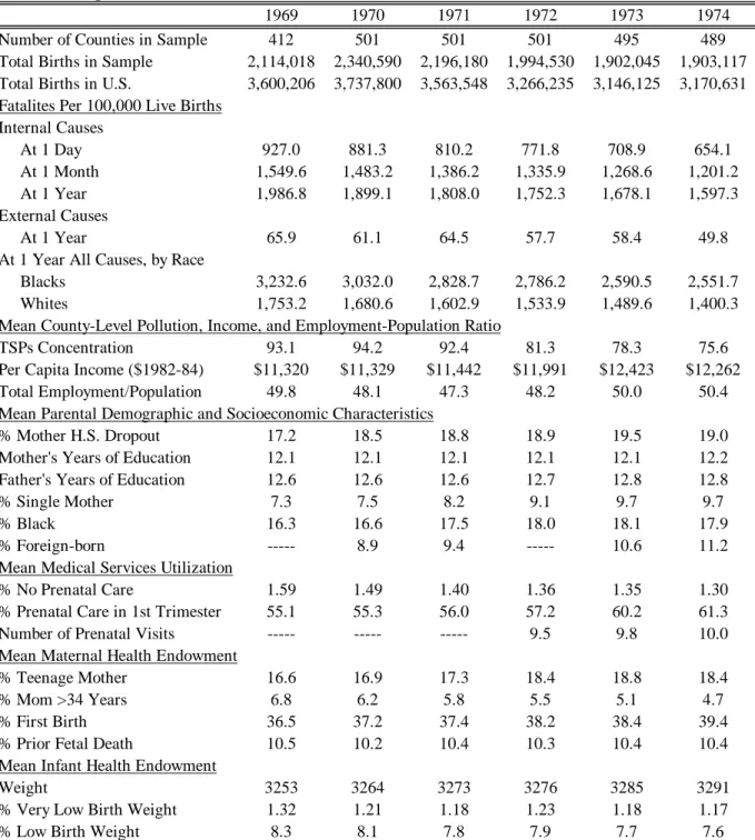
Table 1 presents summary information from 1969-1974 for the 501 counties with available TSPs
and infant mortality data in 1970, 1971, and 1972. This is our primary sample in the below analysis. In
1969 and 1973-74, the sample is further restricted to counties with nonmissing data on TSPs and infant
mortality in those years.
The top rows of the table show that these counties account for over 60% of the 3.2-3.7 million
live births that occur annually in the United States in this period. The next rows present infant fatalities
per 100,000 live births, by cause of death. The internal infant mortality rate in 1971 is 1.8 deaths within a
year of birth per 100 births, while infant deaths due to external causes are much rarer. In 1971, about 45
and 75 percent of all internal infant deaths within a year of birth occur within the first 24 hours and 28
days of birth, respectively. The table also shows national trends in infant mortality, average TSPs
concentrations, and per-capita income across counties. Internal infant mortality rates decreased steadily
from 1969-74. TSPs, on the other hand, fell by over 18 percent from 1971-74, but were relatively stable
from 1969-71. Per-capita income increased by 8.5 percent from 1971-73, before falling slightly from
1973-74, presumably a result of the recession.
The remaining rows of Table 1 present 1969-74 trends for several of the control variables used in
the analysis. Importantly, the magnitude of changes in these variables is small when compared to the
suggest that the average socioeconomic status (SES) of parents was declining from 1969-74, as the
fractions of births to single, high school dropout, and black mothers increased. On the other hand, the
likelihood of a mother receiving prenatal care or having a prenatal visit in the first trimester increased
slightly. The percentage of births attributable to teenagers rose, and the share among women aged 35 and
over fell.21 Finally, the share of first-time births increased slightly while the fraction of mothers who had
a prior fetal death remained stable.
B. Balancing of Observable Characteristics
Before proceeding, we examine whether the nonattainment instrumental variable is orthogonal to
the observable predictors of infant mortality. While it is not a formal test of the exogeneity of the
instrument, it seems reasonable to presume that research designs that meet this criterion may suffer from
smaller omitted variables bias. First, designs that balance the observable covariates may be more likely to
also balance the unobservables (Altonji, Elder, and Taber 2000).22 Second, if the instrument balances the
observables, then consistent inference does not depend on functional form assumptions on the relations
between the observable confounders and infant mortality. Estimators that misspecify these functional
forms (e.g., linear regression adjustment when the conditional expectations function is nonlinear) will be
biased.
Table 2 shows the association of TSPs levels, TSPs changes, and TSPs nonattainment status with
other potential correlates of infant mortality using the same sample of counties as in Table 1. Each
column of the table presents the differences in the variable means between two sets of counties (with
standard errors in parentheses). The first column contains differences in the 1971 levels of the covariates
between counties with high (above the median) and low (below the median) TSPs concentrations in 1971.
If TSPs levels were randomly assigned across counties, one would expect very few significant differences
between the two groups. However, there are significant differences for several key variables, including
21
Rees, et. al. (1996) find that much of the correlation between poor infant health and mother’s age is due to the higher incidence of low birth weight births among teenagers and women 35 and older.
22
For example, in experimental designs testing for differences in the observable characteristics of the treatment and control groups is used to assess whether the treatment was actually randomly assigned.
mother’s race, immigrant status, use of prenatal care, and likelihood of being a teenager. Though not
presented in the table, there are also large and significant differences between the county groups in
per-capita receipts of income maintenance benefits, family assistance payments, and public expenditures on
medical care for low-income individuals (e.g., see Chay, Dobkin, and Greenstone 2003). Overall, these
findings suggest that “conventional” cross-sectional estimates may be biased due to omitted variables.
The next two columns of Table 2 perform a similar analysis for 1971-1972 TSPs changes. They
contain differences in 1971 variable levels and 1971-72 variable changes between counties that had large
(above the median) and small (below the median) reductions in TSPs between 1971 and 1972. These two
county groups exhibit significant differences in the 1971 levels of per capita income, mother’s immigrant
status, prenatal care use, likelihood of being over 34 years old, and pregnancy history. There are also
significant differences in the 1971-72 changes in mother’s and father’s education levels and marginally
significant differences in the changes in the fractions of mothers who are teenagers and who had a prior
fetal death. Thus, fixed effects models may also lead to biased inference.
The next two columns of the table show the differences in 1971 levels and 1971-72 changes
between nonattainment and attainment counties. While nonattainment status is associated with a large
and significant reduction in TSPs concentrations, it is uncorrelated with nearly all of the 1971 levels and
1971-72 changes in the covariates, with the only exceptions being per capita income and mother’s race in
1971. The differences in the changes in mother’s and father’s education and in the changes in the
incidences of mothers who are teenagers and experienced a previous fetal death are greatly reduced by
comparing nonattainment and attainment counties. Also, in contrast to the previous two sets of county
group comparisons, nonattainment and attainment counties exhibit little difference in their receipts of
transfer payments from social programs (results available from the authors). Thus, it appears that the
attainment-nonattainment research design does a better job of balancing the observables.23
23
It should be noted that the composition of counties who are nonattainment and attainment in 1972 is different from the composition of counties with “high” and “low” mean TSPs in 1971 (i.e., column 1).
In the last two columns, the sample is further restricted to the 176 counties with 1970 geometric
mean TSPs concentrations between 60 and 90 µg/m3 – i.e., counties with TSPs levels near the TSPs regulatory ceiling in the regulation selection year. It is evident that focusing on nonattainment and
attainment counties near the regulatory threshold eliminates all of the significant differences in the
covariate levels and changes, including per capita income, mother’s race, and the infant mortality rate in
the year before CAAA enforcement. While nonattainment status is orthogonal to all of the other
covariates, the second row shows that it is still associated with a sharp reduction in TSPs levels between
1971 and 1972 for counties near the regulatory threshold.24 These results provide reassuring evidence on
the quality of the instrumental variables research design used in this study. We probe this further below.
V. Empirical Results A. Cross-Sectional and Fixed Effects Results
First, we replicate the conventional cross-sectional approach to estimating the association
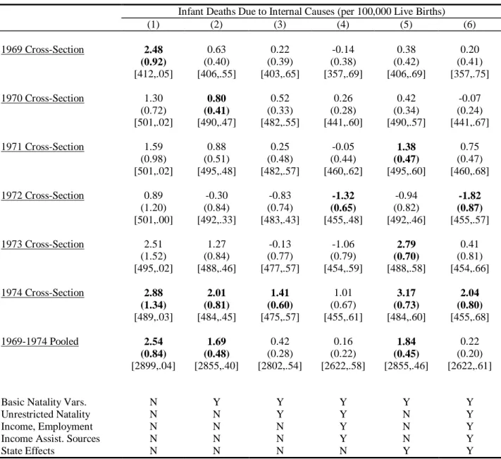
between TSPs pollution and infant mortality that is common in the literature. Table 3 presents the
regression estimates of the effect of TSPs on the number of internal infant deaths within a year of birth
per 100,000 live births for each cross-section from 1969-1974. The final row contains the results for the
pooled 1969-1974 data. Column 1 presents the unadjusted TSPs coefficient; column 2 includes the basic
control variables available in the Natality data; column 3 includes additional Natality variables and
flexible functional forms for the variables; and column 4 further adjusts for per-capita income, earnings,
employment, and transfer payments by source.25 Columns 5 and 6 add unrestricted state effects to the
column 2 and column 4 specifications, respectively. The sample sizes and R2’s of the regressions are
shown in brackets.
There is wide variability in the estimated effects of TSPs, both across specifications for a given
cross-section and across cross-sections for a given specification. While the raw correlations in column 1
24
Given the notation in equations (6) and (7), it should be noted that 1972 nonattainment status is orthogonal to the levels of covariates in 1970 as well (results available from the authors).
25
are all positive, only those from the 1969 and 1974 cross-sections are statistically significant at
conventional levels.26 Including the basic Natality controls in column 2 reduces the point estimates
substantially in most years, even as the precision of the estimates increases due to the greatly improved fit
of the regressions. In addition, only two of the estimates in columns 3 and 4 are significant at
conventional levels, and one of these has a perverse negative sign. This is also true of the most
unrestricted specification in column 6 that also adjusts for state fixed effects.
The largest positive estimates from the cross-sectional analyses imply that a 1-µg/m3 reduction in mean TSPs results in roughly 3 fewer internal infant deaths per 100,000 live births, which is an elasticity
of 0.14. Overall, however, there is little evidence of a systematic cross-sectional association between
particulates pollution and infant survival rates. While the 1974 cross-section produces estimates that are
positive, significant and slightly less sensitive to specification, the 1972 cross-section provides estimates
that are routinely negative. The sensitivity of the results to the year analyzed and the set of variables used
as controls suggests that omitted variables may play an important role in cross-sectional analysis. We
suspect that the fragility of the cross-sectional results to changes in specification and sample is likely to
apply to the estimation of the relationship between other measures of human health (e.g., adult mortality)
and environmental quality (e.g., other air pollutants).
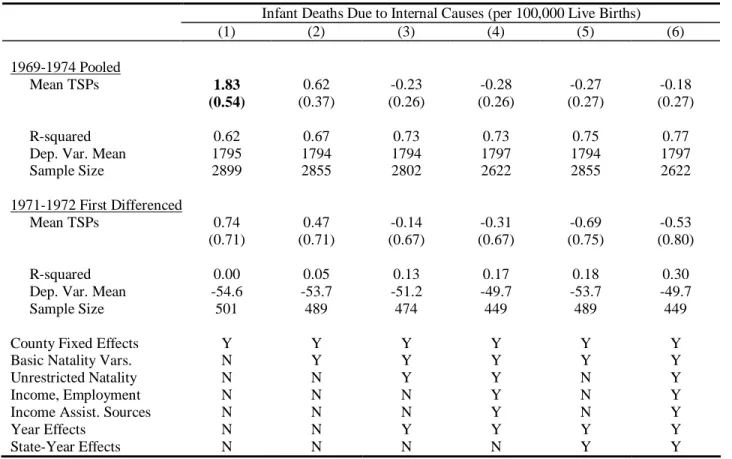
Table 4 presents the fixed effects estimates of the association between mean TSPs and internal
infant mortality rates based on 1969-1974 pooled data (first panel) and 1971-1972 first-differenced data
(second panel). The columns correspond to similar regression specifications as those in Table 3. The
1971-1972 first differences results provide a baseline for comparison to the subsequent instrumental
variables results that use the same samples and control variables. The inclusion of county fixed effects or
the use of first-differenced data eliminates the bias in the cross-sectional estimates attributable to
time-invariant omitted factors that vary across counties. However, these approaches will be biased if there are
unobserved shocks that are correlated with changes in TSPs and infant mortality rates.
26
It is worth noting that the comparison of counties with “high” and “low” 1971 TSPs levels in the first column of Table 2 implies an unadjusted TSPs effect of 2.8 (129.8/45.8), which is 75% greater than the estimated correlation for 1971 in Table 3 (1.6). This is consistent with measurement error in TSPs leading to substantive attenuation bias, since the aggregation in Table 2 “averages out” the measurement errors over many counties.
The 1969-1974 panel shows that the inclusion of county-specific intercepts greatly improves the
fit of the regressions when compared to the pooled cross-sectional regressions in the last row of Table 3.
The raw fixed effects correlation in column 1 is positive and highly significant. However, the estimated
TSPs coefficient falls significantly when the analysis controls for the Natality variables, economic
conditions, transfer payments, year effects and state-year effects. The 1971-1972 first differences results
also suggest little association between changes in TSPs and changes in infant mortality rates.
The fixed effects association between TSPs and infant mortality is small and sensitive to
specification, which is consistent with potential biases due to omitted variables and/or measurement
error.27 We conclude that conventional approaches may not provide reliable estimates of the causal effect
of TSPs on infant mortality and turn our attention to the instrumental variables design outlined above.
B. The Impact of the 1970 Clean Air Act on Air Quality and Infant Mortality
The instrumental variables estimate of the effect of TSPs is a function of two reduced-form
effects: the impact of 1972 nonttainment status on improvements in air quality, and its association with
declines in infant mortality. Here, we provide estimates of the air quality and infant health benefits of the
1970 Clean Air Act and present evidence that our design may plausibly identify the causal effects of
nonattainment status on both outcomes.
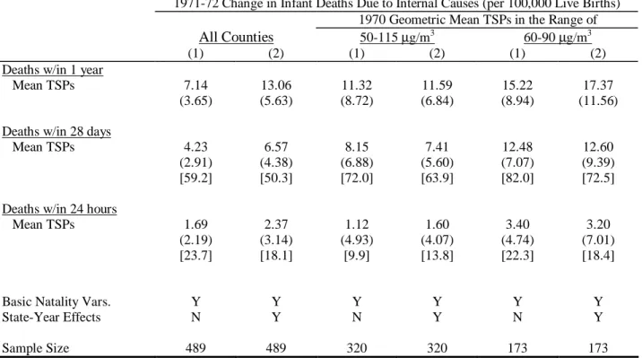
Figure 4 depicts the 1969-1974 time-series of the raw differences in TSPs levels (Panel A) and
internal infant mortality rates (Panel B) between counties that were nonattainment and attainment in 1972.
Separate series are plotted for three samples: 1) all counties with nonmissing TSPs data, 2) the subset of
counties with a 1970 geometric mean TSPs concentration between 50-115 µg/m3, and 3) the subset of counties with 1970 TSPs between 60-90 µg/m3.28 The last two samples are restricted to those counties with TSPs concentrations closer to the 75 µg/m3 regulation ceiling in the regulation selection year.
27
The comparison of counties with “big” and “small” 1971-1972 TSPs reductions in the third column of Table 2 implies an unadjusted TSPs effect of -0.73 (18.8/(-25.6)) for 1971-1972 first differences. This suggests that the small 1971-1972 first-differences estimate in column 1 of Table 4 is not the result of attenuation bias due to measurement error. See footnotes 12 and 26 for more details.
28
The samples consist of the fixed set of counties with continuous monitor readings from 1969-1974. The numbers of counties are 401, 262, and 141, respectively.
Panel A shows large trend breaks in the nonattainment-attainment difference in TSPs that
correspond with the timing of the first year of CAAA enforcement in 1972. There is a clear convergence
in TSPs from 1971 to 1972 even for the subset of counties with 1970 TSPs levels close to the regulatory
threshold. Among counties with 1970 TSPs between 60-90 µg/m3, the 10.5 unit
nonattainment-attainment gap in TSPs in 1971 is almost eliminated by 1972 before rebounding somewhat in 1973. For
counties with 1970 TSPs between 50-115 µg/m3, there is also a significant relative reduction in TSPs from 1971-1972, though the break in trend appears to have started a year earlier than for the other two
county groups. On the whole, the timing and location of the TSPs reductions suggest that enforcement of
the 1970 CAAA led to improved air quality.
Panel B of the figure shows a striking correspondence between the breaks in trend in infant
mortality differences between nonattainment and attainment counties and those in TSPs differences. For
the full sample, the sharp break in infant mortality trends from 1971-1972 matches the break in TSPs
differences. The differential timing of the relative shift down in infant mortality across the three samples
also matches the TSPs patterns. While the full sample and the sample with 1970 TSPs between 60-90 µg/m3 show relative mortality reductions from 1971-1972 only, the sample with 1970 TSPs between 50-115 µg/m3 exhibits a relative mortality reduction the previous year also. Also consistent with the patterns in Panel A, the sample with 1970 TSPs between 60-90 µg/m3 exhibits the largest rebound in relative mortality rates from 1972 to 1973. Below, we show that some of the 1972-1974 rebound in infant
mortality differences is explained by differential changes in the observable characteristics of attainment
and nonattainment counties after 1972.
Taken together, these plots provide evidence of a direct link between regulation-induced
improvements in air quality and reductions in infant mortality rates. First, the timing of the abrupt
declines in TSPs and infant mortality correlate remarkably well across all three groups of counties.
Further, none of the observable covariates, including per-capita income and transfer payments, exhibits
similar trend break patterns in nonattainment-attainment differences. It seems unlikely that any
unobserved factors had nonattainment-attainment differences that changed as sharply or abruptly as the
reduction in mean TSPs leads to 6-14 fewer internal infant deaths per 100,000 live births from
1971-1972, which implies an elasticity between 0.3 and 0.6. The counties with TSPs concentrations closest to
the TSPs regulatory ceiling provide the largest estimate.29
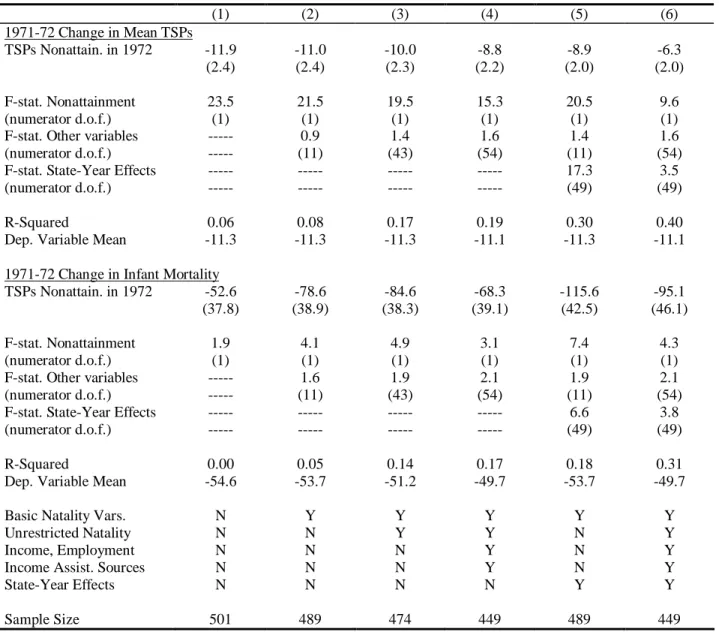
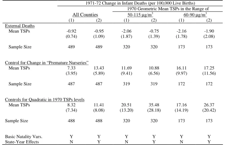
Table 5 contains the regression results from estimating reduced-form equations (5) and (7). The
first panel shows the association between the 1972 nonattainment indicator and changes in mean TSPs
from 1971-1972. The second panel presents the estimated effects of nonattainment status on changes in
infant deaths due to internal causes per 100,000 live births. The columns correspond to the same six
specifications used in Table 4.30
In the first panel, the regulation indicator is associated with a 9-12 µg/m3 reduction in TSPs from 1971 to 1972. This represents a 9-12% improvement in air quality in nonattainment counties and is
similar in magnitude to the effect sizes shown in Figure 4. The estimates are relatively insensitive to the
inclusion of controls for the Natality variables, economic conditions, transfer payments, and unrestricted
state-year effects in columns 1-5. The estimate is reduced in the most unrestricted specification in
column 6, but is still highly significant. In fact, the F-statistics imply that nonattainment status is the most
important (observable) determinant of TSPs changes from 1971 to 1972. The first-stage impact of
regulation is powerful and explains almost all of the overall reduction in mean TSPs in the sample. This
finding contradicts recent research that contends that the CAAAs failed to improve air quality (Goklany
1999).
The second panel reveals another striking empirical regularity. The 1972 TSPs nonattainment
variable is associated with 53-116 fewer infant deaths per 100,000 live births. This implies a 3-6%
decline in the infant mortality rate in nonattainment counties and is similar in magnitude to the implied
effects in Figure 4. The estimates are also generally significant – four of six are significant at the
5-percent level and a fifth at the 10-5-percent level – and tend to increase in magnitude as more controls are
29
Taken literally, the numbers underlying Figure 4 imply that a unit-reduction in TSPs has a larger marginal effect at TSPs concentrations just above the 75-µg3 regulatory ceiling than at higher concentrations.
30
It should be noted that the specifications for columns 1 and 2 of Table 4 do not control for year effects, whereas columns 1 and 2 of Table 5 do include a constant to absorb year effects in the first differences. For 1971-1972 first-differences, the estimates in columns 1 and 2 of Table 4 that include a constant are –0.40 (0.71) and –0.36 (0.67).
added. This is particularly notable given the unpredictability of changes in infant mortality rates. In
column 3, for example, only the coefficients on the indicators for twins or greater birth and mother’s race
have t-ratios similar in magnitude to the t-ratio for the nonattainment coefficient.31
These results imply that the Clean Air Act regulations resulted in substantial reductions in infant
mortality in nonattainment counties. The weighted average of the estimates (with weights equal to the
inverse of the sampling errors) suggests that relative to attainment counties nonattainment counties had 82
fewer infants deaths per 100,000 births. Multiplying this figure by the 1.52 million births that occurred in
nonattainment counties in 1972 implies that 1,300 fewer infants died in 1972 than would have in the
absence of the 1970 Act.
Figure 5 presents the raw and regression adjusted trends in differences between attainment and
nonattainment counties in TSPs (Panel A) and infant mortality (Panel B) from 1969 to 1974. The graph
plots the estimated coefficients on interactions of 1972 nonattainment status with year indictors from
regressions that also include year main effects. The Adjust 1, Adjust 2, and Adjust 3 series are based on
specifications that respectively use the same controls as in columns 2-4 of Table 5.32 Panel A of the
figure shows that regression adjustment has little effect on the size of the trend break in relative TSPs in
nonattainment counties after 1971.
Panel B shows that regression adjustment also has little effect on the size of the relative infant
mortality reduction from 1971 to 1972 and, if anything, tends to increase the measured improvement in
nonattainment counties. Covariate adjustment does however have a substantial effect on the levels of the
nonattainment-attainment mortality differences in the pre-regulation period, 1969-1971. Importantly, it
also reduces the magnitude of the rebound in relative mortality rates from 1972 to 1974, suggesting that
some of the rebound is due to a worsening in the observable characteristics of nonattainment counties
relative to attainment ones. Appendix Figure 1, which plots the predicted mortality differences between
31
Being black and having a twins or greater birth are both associated with higher rates of infant death. The estimated coefficients on almost all of the other variables (e.g., parents’ socioeconomic characteristics, mother’s prenatal care use and pregnancy history) are statistically insignificant.
32
The regressions use the pooled 1969-1974 data and restrict the effects of the control variables to be constant over time. The sample is the fixed set of 401 counties with continuous TSPs readings from 1969-1974.
nonattainment and attainment counties based on the Adjust 3 regression specification excluding TSPs,
confirms this conclusion.33 It shows that in the absence of the TSPs changes, the
nonattainment-attainment mortality gap would have been predicted to widen over the period due to the general
worsening of the relative characteristics of nonattainment counties.
These findings suggest that while the observable controls are strong predictors of infant mortality
levels, they cannot account for the sharp mortality change in nonattainment counties from 1971 to 1972.
Interestingly, Figure 5 also explains the differences across cross-sections in the estimated TSPs
coefficients in Table 3. In 1972, for example, nonattainment counties had higher TSPs levels than
attainment counties but lower infant mortality rates once differences in observable predictors are
controlled for. This corresponds with the perverse, negative estimates for the 1972 cross-section in Table
3. The nonattainment-attainment differences in TSPs and infant mortality in 1974 also correspond with
the systematically positive estimates for the 1974 cross-section. In fact, much of the across-year variation
in the cross-sectional estimates in Table 3 appears to be due to the sharp improvement in air quality
caused by the Clean Air Act.
Our final assessment of the causal impact of the 1970 Act on air quality and infant mortality
exploits the discontinuity in the assignment rule that determines 1972 nonattainment status. Figure 6
graphs the bivariate relations of both the 1971-1972 change in TSPs and the 1971-1972 change in infant
mortality with the geometric mean of TSPs levels in 1970 (the regulation selection year). The plots come
from the estimation of nonparametric regressions that use a uniform kernel density regression smoother.
Thus, they represent a moving average of the raw changes across 1970 TSPs levels.34 This graphical
analysis allows us to test whether there are sharp differences in the outcomes that correspond with the
discrete zero-to-one change in the probability that a county was designated nonattainment at the
33
Appendix Figure 1 was constructed from two steps: 1) a regression of infant mortality rates on the observables excluding TSPs; and 2) a regression of the predicted infant mortality rates from the first regression on year effects and interactions of the year effects with 1972 nonattainment status. Thus, the figure provides a “single-index” summary of the differences between nonattainment and attainment counties in the observable confounders. 34
regulatory ceiling (the vertical line in the figure) mandated by the CAAA. Recall, counties with 1970
geometric mean TSPs levels below (above) 75 µg/m3 are attainment (nonattainment) in 1972.35 For the full set of counties in our primary sample, the figure confirms the regression results in
Table 5. Nonattainment counties with 1970 TSPs levels above the regulatory ceiling had much larger
reductions in both mean TSPs and infant mortality rates from 1971-1972 than their attainment
counterparts with 1970 TSPs below the ceiling. The most striking features of the graph, however, are the
clear “trend breaks” in TSPs and infant mortality rate changes at the regulatory threshold. These breaks
strongly suggest that the CAAA regulation is a causal factor in improvements in both outcomes for
nonattainment counties.
Focusing on the counties with geometric mean TSPs between 50 and 100 µg/m3 in 1970, there is a clear association between larger reductions in mean TSPs and greater decreases in infant mortality at the
EPA-mandated air quality standard. The correspondence of the trend breaks implies that our research
design may identify the casual effect of air pollution on infant mortality through the mechanism of
regulation. This “nonparametric” display of the data suggests instrumental variables estimates that are
similar in magnitude to the two-stage least squares estimates presented in the next section.
On the other hand, there appear to be secular decreases in infant mortality rate reductions at 1970
TSPs levels well below (30-50 µg/m3) and well above (100-150 µg/m3) the 75-µg/m3 threshold. Thus, IV estimates based on the subsample of counties close to the regulation discontinuity will be larger in
magnitude than those based on the entire sample. This could be due to either a nonconstant infant
mortality-TSPs gradient or greater differences in the characteristics of nonattainment and attainment
counties with 1970 TSPs levels far away from the discontinuity.
Figure 7 provides two checks of the validity of the 1972 nonattainment research design. First,
Panel A of the figure empirically examines the validity of the “smoothness” condition discussed above. It
plots the infant mortality changes predicted by the observable covariates excluding TSPs changes, E[(yc72
35
The six counties that were nonattainment in 1972 for exceeding the daily concentration standard but not the annual geometric mean standard in 1970 are dropped from the analysis. Thus, the sample contains 264 nonattainment counties and 230 attainment counties.
yc71)|(Xc72-Xc71)], along with the actual infant mortality changes from Figure 6, as a function of 1970 TSPs
levels. The predicted changes come from a regression that includes the full set of Natality control
variables – i.e., column 3 of Table 5.
The figure shows that this index of the non-pollution determinants of infant mortality changes is
smooth at the regulatory threshold. By contrast, actual infant mortality rates fall substantially at the
threshold, presumably due to the large TSPs reductions. The mortality predictors do appear to explain the
decreasing reductions in infant mortality at low 1970 TSPs levels. But for counties with 1970 TSPs
greater than 55-60 µg/m3, there is little association between predicted mortality changes and pre-regulation TSPs levels. Consistent with the results in Table 2, this finding suggests that attainment and
nonattainment counties in the neighborhood of the regulatory ceiling have the same characteristics. In
addition, the only observable variable that exhibits a break at the ceiling that corresponds with the infant
mortality break is the change in TSPs.
Panel B of Figure 7 plots pre-regulation changes in infant mortality and mean TSPs from
1969-1970 by the geometric mean of TSPs in 1969-1970. This figure provides the following falsification test. Since
the 1970 Clean Air Act was not yet in force, there should not be a “trend break” in 1969-1970 changes in
the outcome variables near the 75-µg/m3 threshold. The graph shows that pre-regulation changes in infant mortality and TSPs have a smooth relation with 1970 TSPs levels at the regulatory ceiling. This is
consistent with 1972 nonattainment status being the cause of the 1971-1972 outcome changes. In fact,
before the passage of the 1970 CAAA, nonattainment counties had rising TSPs levels relative to
attainment counties, which corresponds with the growing gap in infant mortality in the pre-regulation
period. These patterns are consistent with the more aggregated patterns in Figure 4.
Taken together, Figures 4-7and Table 5 provide convincing evidence that the 1970 CAAA had
significant air quality and infant health benefits. The results imply that the regulation of nonattainment
counties in 1972 resulted in a 10 percent reduction in TSPs concentrations and a 4-5 percent decline in
infant mortality rates from 1971 to 1972. Further, the nonattainment design allowed us to develop several
credible tests of the causality of the CAAA intervention and of the infant mortality-TSPs relation. Tests