Adaptive control of time delay systems and applications to automotive control problems

Adaptive Control of Time Delay Systems and

Applications to Automotive Control Problems

by

Yildiray Yildiz

Submitted to the Department of Mechanical Engineering

in partial fulfillment of the requirements for the degree o

Doctor of Philosophy in Mechanical Engineering

at the

MASSACHUSETTS INSTITUTE OF TECHNOLOGY

MASSACHUSETTS INSTITUTE O TECHNOCLOGY

MAR 0 6 09

K1

t

IE--S

February 2009

@ Massachusetts Institute of Technology 2009. All rights reserved.

Author ...

Department of Mechanical Engineering

January 26, 2009

Certified by...

...

Anuradha Annaswamy

Senior Research Scientist

Thesis Supervisor

Accepted by ...

...

David Hardt

Chairman, Department Committee on Graduate Theses

Adaptive Control of Time Delay Systems and Applications

to Automotive Control Problems

by

Yildiray Yildiz

Submitted to the Department of Mechanical Engineering on January 26, 2009, in partial fulfillment of the

requirements for the degree of

Doctor of Philosophy in Mechanical Engineering

Abstract

This thesis is about the adaptive control of time delay systems with applications to automotive control problems. The stabilization of systems involving time delays is a difficult problem since the existence of a delay may induce instability or poor performance for the closed loop system. A unique approach for controlling systems with known time delay was originated by Otto Smith in the 1950s by compensating for the delayed output using input values stored over a time window of [t - T, t] and

estimating the plant output using a model of the plant. Later, this idea was extended to include unstable plants as well, using finite-time integrals of the delayed input values thereby avoiding unstable pole-zero cancellations that may occur in Smith's controller. Adaptive versions of these delay compensating controllers were also de-veloped with rather complicated adaptive rules which might not be practical to use in real applications. In this thesis, a simpler adaptive version of delay compensating controllers is developed, which has adaptive rules that are easily implementable and thus suitable for real life implementations. The developed controller is tested in two important automotive control problems that are idle speed control (ISC) and fuel-to-air ratio (FAR) control. These two applications, ISC and FAR control, constitute the experimental part of this research.

In ISC, the objective is to regulate the engine speed to a prescribed set-point in the presence of accessory load torque disturbances such as due to air conditioning and power steering. The adaptive controller, integrated with the existing proportional spark controller, is used to drive the electronic throttle actuator. Both simulation and experimental results demonstrating the performance improvement by employing the adaptive controller are presented. Modifications and improvements to the controller structure, which were developed during the course of experimentation to solve specific problems, are also presented. In addition, the potential for the reduction in calibration time and effort which can be achieved with our approach is discussed.

The objective in FAR control is to maintain the in-cylinder FAR at a prescribed set point, determined primarily by the state of the Three-Way Catalyst (TWC), so that the pollutants in the exhaust are removed with the highest efficiency. The FAR

controller must also reject disturbances due to canister vapor purge and inaccuracies in air charge estimation and wall-wetting (WW) compensation. Two adaptive controller designs are considered. The first design is based on feedforward adaptation while the second design is based on both feedback and feedforward adaptation. Both simulation and experimental results demonstrating the performance improvement by employing the APC are presented. In addition, modifications and improvements to the APC structure, which were developed during the course of the experiments, to solve specific implementation problems are presented.

Thesis Supervisor: Anuradha Annaswamy Title: Senior Research Scientist

Acknowledgments

Dr. Anuradha Annaswamy. You may not know, but when I first come to your office to express my interest in your work, I had little hope that you would offer me a research assistant position. I was very interested in controls but I was about to turn back home with all my dreams in my bag, due to lack of funding. You are the one who enabled me to follow my dreams, stay at MIT, conduct great research, complete this thesis and, finally, pursue my passion by getting an offer from NASA for my postdoctoral studies. Thank you.

Dr. Ilya Kolmanovsky. Your encouragement during tough times and your moti-vation during good times provided me enough fuel to complete this research. Your comments like "Great work!" have always made me feel that I'm responsible to really deserve these words. Thank you for always supporting me.

Dr. Diana Yanakiev. After the first few days that I spent with you, it was clear to me that you would not accept anything less than my best from me. I believe that I was very lucky to work with a mentor who was as demanding as you, always focused and always honest and critical, in a good way, to my work. Thank you.

Professor Kamal Youcef-Toumi and Professor Ahmed F. Ghoniem. I would like to thank you for serving as my committee members although you have a very busy schedule. You always made me think about the important points that I was otherwise not considering and you played a critical role in making this research as rigorous as possible.

Professor Mustafa Unel. Again, thank you for your support, encouragement, motivation, teaching and coaching. Most importantly, thank you for always trusting me.

Dr. Davor Hrovat of Ford Motor Company. Thank you for your support and encouragement. Chris Teslak and Steve Magner of Ford Motor Company. Thank you for your help with the experimental setup and for valuable discussions.

My labmates Dr. Jinho Jang, Travis Gibson, Zachary T. Dydek, Manohar Srikanth and Megumi Matsutani. Thank you for providing a cozy and enjoyable studying

en-vironment, and thank you for your friendship.

Dr. Zekeriyya Gemici. Thank you for being my friend and for challenging me on almost all subjects we can find to talk about. You are among the few people that I resonate with the same frequency. And of course, thank you for your contribution of 10 pounds to my body weight after all those sundae sessions.

Tugba Uzer. You are my inspiration and my passion. Thank you for your exis-tence.

My whole family. Tugba, thank you for being a wonderful sister. Abutel Hala and Gulderen Hala, thank you for your unconditional love and support. Nene, thank you for your prayers. Mom and dad, thank you for being great parents. Thank you for your constant encouragement and support and love. I'm very lucky to be a member of this big family.

Contents

1 Introduction

1.1 Adaptive Posicast Control (APC) . ... 1.2 Idle Speed Control (ISC) ...

1.3 Fuel-to-Air Ratio (FAR) Control . ...

2 Adaptive Posicast Control Theory 2.1 First-Order Plant . . ...

2.1.1 The Posicast Controller . ...

2.1.2 The Adaptive Posicast Controller . . . . . 2.2 State variables accessible ...

2.3 Adaptive Posicast Control in the presence of inpi ments with n* < 2 ...

2.3.1 Exact model matching for delayed systems 2.3.2 Adaptive Controller . ...

2.3.3 Stability Analysis ...

2.3.4 Possible Nonlinear Extention . . . . 2.4 Summary . . . ... 23 .. . . . 23 .. . . . 24 . . . . . . 25 .. . . . 27 ut-output measure-. . . . .. . 28 . . . . . 29 .. . . . . 32 .. . . . 36 .. . . . 45 ... . . . 47 3 Spark Ignition Engine Idle Speed Control:

An Adaptive Control Approach

3.1 Plant Model .... ... ...

3.1.1 Throttle Mass Flow . .. ... 3.1.2 Intake Manifold ...

49 49 49 50

3.1.3 Engine Air Mass Flow . 3.1.4 Torque Generation ... 3.1.5 Engine Rotational Dynamics . 3.1.6 Final Model for ISC ... 3.2 APC Design ...

3.2.1 Initial Design ...

3.2.2 Implementation Enhancements 3.2.3 Final Design and Calibration 3.3 Simulations ... 3.4 Experiments ... 3.4.1 Set-point Tracking ... 3.4.2 Disturbance Rejection . . 3.4.3 Robustness ... 3.5 Summary ...

4 Spark Ignition Engine Fuel-to-Air Ratio Control: An Adaptive Con-trol Approach

4.1 Plant Model ...

4.1.1 Wall-Wetting (WW) Dynamics ...

4.1.2 FAR Formation and Propagation to the UEGO Sensor . .

4.1.3 Sensor Dynamics ...

4.1.4 Reduced Order Model ... 4.2 Controller Design ...

4.2.1 Baseline Controller ...

4.2.2 Adaptive Feedforward Controller (AFFC) ... 4.2.3 Adaptive Posicast Controller (APC)

4.2.4 Implementation Enhancements ... 4.2.5 Final Design and Calibration ... 4.3 Simulation and Experimental Results . ...

4.3.2 APC vs. Baseline Controller ... .. ... 87 4.3.3 APC vs. Gain-Scheduled Smith Predictor . ... 92

4.4 Summary ... ... .. 94

5 Summary and Future Research 97

A The Bound on the Series S 101

B Disturbance Rejection Proof 103

C Memory Requirements and Computational Complexity 105

List of Figures

1-1 TWC efficiency vs. air-to-fuel ratio. . ... . . . 19

2-1 Exact model matching, Controller NC. . ... ... . 30

2-2 Exact model matching, Controller C. ... ... . 32

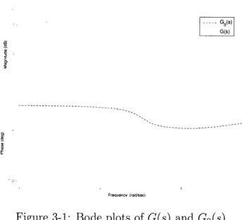
3-1 Bode plots of G(s) and Go(s) ... . ... . 52

3-2 Nonlinear model set-point tracking. Adaptation rates are calculated using (3.27) with no further tuning. ... . ... . 63

3-3 Nonlinear model set-point tracking. z, = Zr = 1, Zy = 220. ... . 63

3-4 Rapid prototyping with MicroAutoBox using CAN. . ... 64

3-5 Comparison of the baseline controller with adaptive controller for set-point tracking. Fw is the same used in the simulation shown in Fig. 3-3 65 3-6 Comparison of the baseline controller with adaptive controller for power steering disturbance rejection at 650 rpm. Fw is the same used in the simulation shown in Fig. 3-3 ... ... . 66

3-7 Comparison of the baseline controller with adaptive controller for power steering disturbance rejection at 900 rpm. Fw is the same used in the simulation shown in Fig. 3-3 ... ... . . . . . 66

3-8 Comparison of the baseline controller with adaptive controller for power steering disturbance rejection at 590 rpm. Lw is the same used in the simulation shown in Fig. 3-3 ... ... ... . .. 67

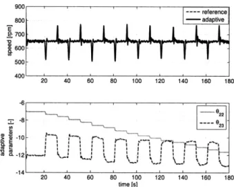
3-9 Top figure: Adaptive controller performance for power steering distur-bance. Bottom figure: Evolution of the controller parameters. .. .. 68

3-10 Top figure: Adaptive controller performance for power steering dis-turbance. Bottom figure: Evolution of the controller parameters with

o-modification. . ... 68

4-1 Plant block diagram representation. . ... 72

4-2 Overall closed loop controller structure. . ... 75

4-3 Inner-loop structure with AFFC. ... ... 77

4-4 Rapid prototyping with MicroAutobox using CAN. . ... 84

4-5 Comparison of baseline controller and AFFC. a) Response to a set-point change b) Response to purge disturbance . ... 86

4-6 Baseline controller vs. AFFC a) 4 and air flow rate when baseline controller is active b) ( and air flow rate when AFFC is active c) Engine speeds d) Purge fuel flow rates. . ... . . 88

4-7 Comparison of baseline controller with APC for purge disturbance re-jection at 700 rpm. .... ... . . ... ... . .. 89

4-8 Comparison of baseline controller with APC for purge disturbance re-jection at 1000 rpm, with c = 1. ... ... .. . . 89

4-9 Time histories of a) (, b) Engine speed c) Engine relative air flow, d) Tracking error integral, during vehicle acceleration and deceleration for APC vs. baseline controller, with c = 1.. ... 90

4-10 Comparison of baseline controller with APC during vehicle accelera-tion, with c = 1.5. ... 91

4-11 Time histories of a) 1 b) Engine relative air flow c) Feedback con-trol input d) Tracking error integral, during vehicle acceleration and deceleration for gain-scheduled SP vs. APC, with c = 1.5... .. 93

4-12 Comparison of SP and APC for input step disturbance rejection in the presence of sensor time constant uncertainty. . ... 95

4-13 Comparison of SP and APC for input step disturbance rejection in the presence of sensor time constant and delay uncertainty. . ... 95

Chapter 1

Introduction

1.1

Adaptive Posicast Control (APC)

A time delay can be defined as the time interval from the application of a control signal to any observable change in the measured variable [1]. Time delays are ubiquitous in dynamical systems, present as computational delays, input delays, measurement delays and transportation/convection lags to name a few. In addition, higher order dynamical systems can often be modeled by low order systems plus a time delay. Many examples of systems including time delays, such as chemical, biological, mechanical, physiological and electrical systems, are given in [2] and [3]. Detailed surveys of time delay systems can be found in [4] and [5].

The stabilization of systems involving time delays is a difficult problem since the existence of a delay may induce instability or bad performance for the closed loop system. In many controller designs, the delay is neglected and stability and robustness margins are given with respect to delay. The same approach can also be found in some adaptive control designs [6]. However, in general, these approaches produces small delay margins.

A unique approach, called the Smith Predictor (SP), was originated by Otto Smith in the 1950s to solve the problem of controlling the systems with large delays [7]. The main idea in this approach is predicting the future output of the plant, using a plant model, and using this prediction to cancel the effect of the time delay. This

future prediction inspired the name for the "posi-cast", which stands for "positively (fore)casting". This is different from the feedforward control technique, also known as posicast control, used to cancel the oscillatory behavior of lightly damped systems. See also [8], [9], [10] and [11] for improvements and modifications on SP ideas. SP method, however, is not suitable for unstable systems due to the possibility of unsta-ble pole-zero cancellations. A method, called finite spectrum assignment (FSA), that works also for unstable systems was introduced by Manitius and Olbrot, where the main contribution was using finite time integrals to prevent unstable pole zero cancel-lations [12]. _{See also [13], [14] and [15] for FAS techniques. An analogous solution in}

frequency domain is given by Ichikawa in [16]. Although these approaches solve the problem of controlling time delay systems, their success depends on accurate plant models. In reality, it is not easy to obtain reliable plant models and, in general, the plant parameters contain a degree of uncertainty. In addition, these parameters may change over time. Addressing this problem, in [17], Ortega and Lozano introduced an adaptive version of these delay compensating controllers using an augmented error approach [18]. Although this controller introduces adaptation and removes the need for accurate plant models, it has high complexity. A simple controller is generally more advantageous if it is meant to be used in industrial applications, especially in mass production implementations. In addition, the plant poles are restricted to mul-tiplicity one in this controller. In [19], a simpler adaptive design, called Adaptive Posicast Controller (APC) is given with the same plant pole restriction. In this the-sis, a rigorous treatment of the APC is given without any restrictions on plant pole multiplicities, and carefully addressing the necessary technical details.

As mentioned above, the APC is suitable for industrial applications due to its sim-plicity and low computational requirement. These features are important especially in the mass production applications such as automotive engine control. Triggered by the governmental regulations on emissions in 1960's and 1970's, the introduction of the microprocessor-based control permitted the automotive manufacturers to design cleaner, more fuel efficient, better performing and more reliable powertrain systems. The associated control problems provide continuing challenges to control engineers as

the requirements progressively become more stringent. Higher levels of performance and robustness are expected, while the calibration time and effort need to be reduced. Advances in control theory can be exploited to address these challenges. See [20] for an introduction to modeling and control of internal combustion engines.

In this research, we applied the APC to two important automotive control prob-lems: the idle speed control (ISC) problem and the fuel-to-air ratio (FAR) control problem. In both of these applications, the APC performed better than the base-line controllers that are existing in the test vehicles. These two control problems are explained in detail below.

1.2

Idle Speed Control (ISC)

The basic problem of Idle Speed Control (ISC) is to maintain the engine speed at a prescribed set-point in the presence of various disturbances such as due to air conditioning, transmission engagement or power steering accessory load torques [21]. There are several well-known challenges in this control problem, one of the most important of which is the time-delay between the intake event and combustion event of the engine. This time delay limits the achievable performance in the electronic throttle control loop. The second challenge is that the controller performance must be robust to changes in the idle speed set-point, to changes in operating conditions

(varying altitude, engine temperature and/or ambient temperature, etc.) and to part-to-part and aging-caused variability. Finally, obtaining an accurate and simple model which is appropriate for control design can be both difficult and time-consuming.

Idle Speed Control has been a classical problem in automotive control, and the celebrated Watt's governor (1796) was, in fact, a speed controller for a steam en-gine. Even though ISC is implemented in most of the vehicles on the road today, increasingly stringent regulatory and customer requirements necessitate its continu-ing improvement. For instance, a better performcontinu-ing ISC can improve fuel economy by reducing spark reserve and lowering idle speed set-point, and it can also accommodate changes in sensors and actuators (e.g., a replacement of an air-bypass-valve by the

electronic throttle or reduction in sensor or actuator cost). Finally, ISC designs that can lower calibration time and effort can help reduce time-to-market, which is a key priority for automotive manufacturers.

The ISC problem is typically addressed by combining some form of a feed-forward control with a closed-loop compensation based on the engine speed error. The feed-forward controller may consist of multiple look-up tables which may, for instance, predict the loads due to accessories for different operating conditions. A closed-loop controller determines the compensation with electronic throttle and spark timing ac-tuators for the engine speed tracking error and is typically gain-scheduled on operating conditions where nonlinear maps may be used to determine the gains. The major ef-fort in the calibration, which is the process of tuning control system parameters, is spent in determining the gains of the feed-forward controller. One of the reasons for this may be due to the low capability of the closed loop controller, which in turn shifts the burden of compensation to the feed-forward controller.

Many different closed loop designs have been proposed in the literature includ-ing -I control [22], t2 control [23], slidinclud-ing mode control [24], [25], fl optimization [26], feedback linearization [27], proportional-integral (PI) and proportional-integral-derivative (PID) control [28], [29], [30], [31], [32], linear quadratic control (LQ) [33], [31], [34], model predictive control (MPC) [35], adaptive control [36], [37], [38] and estimation based control [39], [40], [41], to name a few. A comparison between dif-ferent control algorithms for the idle speed control problem can be found in [42]. A comprehensive survey of engine models and control strategies developed for ISC can be found in [21].

The literature, given above, about classical and advanced control applications to the ISC problem, proves the continuing interest in an automated, model based control approach, and our work built upon these results by eliminating the need of a pre-cise engine model for classical or optimization based algorithms and by reducing the conservatism introduced by the robust control approaches. This is achieved by using the Adaptive Posicast Controller (APC) developed in this thesis [19], [43], which is an adaptive controller for time delay systems. Successful adaptive control approaches

are presented also in references [36], [37], [38], but our approach is different from these: In [36], the adaptation is used to select the idle speed set point and in [37], the torque differences among the cylinders are estimated to reduce the short term fluctuations caused by them. Finally, in [381, simulation results of idle speed control by online estimation of the plant parameters and using these estimates in the control scheme using two actuators, spark and bypass valve, are given. In our approach, we apply the APC, a model reference adaptive controller developed for time delay systems, to control the idle speed at a prescribed set-point, in the presence of exter-nal disturbances, like power steering disturbance, and uncertainties due to modeling inaccuracies and operating point changes. We do not employ an online parameter estimation algorithm which may require additional computation power. In addition, we present experimental results demonstrating the improvements of the algorithm over the baseline controller existing in the vehicle, as well as the robustness of the algorithm by showing the parameter evolution during the course of the experiment.

The APC approach addresses the key challenges due to uncertainties and time delay that are important for ISC application. The underlying control architecture includes several components including the classical Smith Predictor [7], its variant reported in [12] based on finite-spectrum assignment, and adaptation [16], [17]. The controller is modified from its original design to take care of the specific needs of the idle speed control application and additional design methods are developed to facilitate the controller deployment: Firstly, an algorithm is developed for the adap-tation rate selection. Secondly, a fine-tuning method is introduced to minimize the controller tuning. Finally, a robustifying scheme is used to prevent the drift of the adaptive parameters. Our main contribution is the demonstration of the potential of this adaptive controller to improve the performance and to reduce the time and effort required for the controller calibration. This is achieved by the help of modifications and improvements that are listed above.

The experimental results obtained using Ford F-150 test vehicle demonstrate the capability of the controller to improve performance and decrease the calibration time and effort.

Adaptive Posicast ISC approach represents a step towards a fully self-calibrating ISC because less reliance on feed-forward characterization of accessory loads is re-quired, and because the controller gains are automatically tuned online.

While our control approach is adaptive, its development both benefits from and depends on the structural properties of the underlying plant model. This plant model for ISC control is briefly discussed in Chapter 3, while the reader is referred to [20] for a more extended treatment of the underling modeling techniques.

1.3

Fuel-to-Air Ratio (FAR) Control

The Fuel-to-Air Ratio (FAR) control is one of the most important control problems for conventional gasoline engines. The FAR control performance can strongly impact key vehicle attributes such as emissions, fuel economy and drivability. For instance, the FAR in engine cylinders must be controlled in such a way that the resulting exhaust gases can be efficiently converted by the Three-Way Catalyst (TWC). The TWC efficiency is about 98 percent when the fuel is matched to air charge in ex-actly stoichiometric proportion and drops abruptly outside a narrow region as seen in Fig. 1-1 [44]. The TWC can also compensate for the temporary FAR deviation from stoichiometry, by either storing excess oxygen or releasing oxygen to convert oxides of nitrogen (NOx), excess hydro-carbons (HC) and carbon monoxide (CO). Thus, for the TWC to operate efficiently, the stored oxygen level must be regulated so that a range to accommodate further release or storage during transient conditions is available [20]. The oxygen storage level in the TWC may be inferred on the basis of the TWC model and a signal from a switching Heated Exhaust Gas Oxygen (HEGO) sensor located downstream of the TWC. In addition, the oxygen storage capacity of the TWC depends on the size and precious metal loading of the TWC. Therefore, if the FAR excursions and their durations are reduced with a well-performing controller, the storage capacity of TWC and its cost may be reduced as well.

A conventional FAR control system includes two nested controllers. The outer-loop controller generates a reference FAR (set-point) for the inner-outer-loop controller

100 ... z 80 W 60 z /

o

Figure 1-1: TWC efficiency vs. air-to-fuel ratio.

based, for instance, on the deviation of the estimated TWC stored oxygen state. The inner-loop controller maintains the FAR upstream of the TWC at this set-point by using the measurements of the feedgas FAR with a linear Universal Exhaust Gas Oxygen (UEGO) sensor to appropriately correct engine fueling rate. Small amplitude low frequency periodic modulation may be superimposed over the set-point to further improve catalyst efficiency. The HEGO sensor downstream of the TWC is also used to improve robustness to UEGO sensor drifts, changes to fuel type, and for diagnostics.

The inner loop controller consists of a feedforward component which is fast but may not be always accurate, and a feedback component which is slower but eliminates the steady-state error [20]. The feedforward component consists of estimation of the air and fuel path dynamics combined with appropriate compensations. These air and fuel dynamics correspond, mainly, to the intake manifold lag that affects the air charge, and the wall-wetting (WW) that determines the amount of fuel inducted into the cylinder for each fuel injection event during transient operation.

The FAR control problem has been extensively investigated over many years. In terms of advanced approaches, here we mention the use of nonlinear feedforward

controllers [45], adaptive controllers [46], [47], [48], [49], feedback linearization [50], observer based controllers [51], [52], [53], sliding mode controllers [54], [55], [56], lin-ear quadratic regulators [57], [58], H, controllers [59], [60], Smith Predictors [61], neural network controllers [62] and model predictive controllers [63]. The use of an electronic throttle as an additional control actuator [64] or secondary/port throttles [65] has also been explored. Apart from stoichiometric FAR controllers, reference [66] considers control of FAR in a lean burn engine using linear parameter-varying controllers. In addition to these, reference [67] presents an interesting example of es-timating the FAR in the cylinders without using the oxygen sensor and thus reducing the time delay in the system, and [68] considers estimating the fuel-film dynamics. The motivation for these and related studies has been to achieve improved perfor-mance and robustness of the FAR control thereby enabling emission, fuel economy and drivability improvements.

Main challenges in the design of the FAR controller include variable time delay, uncertain plant behavior and disturbances. The time delay in the system comprises two basic components [66]: the time it takes from the fuel injection calculation to exhaust gas exiting the cylinders and the time it takes for the exhaust gases to reach the UEGO sensor location. The time delay in the system is a key factor limiting the bandwidth of the FAR feedback loop. The plant uncertainties are the result of inaccuracies in the air charge estimation and in the WW compensation, as well as changes in the UEGO sensor due to aging. When the carbon canister, which stores the fuel vapor generated in the fuel tank, is purged, the fuel content in the purge flow into the intake manifold is also uncertain and creates disturbance to the FAR control loop.

We, therefore, are interested in a control approach which can handle both uncer-tainties and large time-delays, and that can achieve high performance. The literature, given above, about classical and advanced control applications to the FAR control problem demonstrates continuous interest in an automated, model based control ap-proach, and our work is built upon these results by eliminating the need of a precise engine model for classical or optimization based algorithms and by reducing the

con-servatism introduced by the robust control approaches. This is achieved by using the Adaptive Posicast Controller (APC) [19], [43], which is an adaptive controller for time delay systems. Successful adaptive control approaches are presented also in references [46], [47], [48] and [49], but our approach is different from them: In [46] and [48], a nonlinear least squares parameter identification method is used to identify the plant parameter values online and then these values are used in the controller. For the convergence of these parameters, the condition of persistent excitation is needed. In addition, this online parameter identification may require extra computational power. In both of the references, the controllers are applied to a single cylinder laboratory engine. In [47], again a similar approach is taken where an extended Kalman Filter is used to identify the plant parameter values online. Similarly, in [49], the authors use a step by step experimental procedure to identify the sensor time constant, during the time of operation, where a rich input excitation is needed for parameter convergence.

Our approach is based on direct adaptation where an online parameter identification scheme is not used. In addition, we apply the APC to a Lincoln Navigator test ve-hicle with 8 cylinders, which makes the control task much harder due to cylinder to cylinder and bank-to-bank variations. Finally, in our work, we do not only present our results but also give a comparison with the existing control design in the test vehicle and with a gain scheduled Smith Predictor.

The Adaptive Posicast Control (APC) is a recently developed control design ap-proach that is especially suited for plants with large time-delays [19], [43] and para-metric uncertainties. The APC can be described as an adaptive controller that com-bines explicit delay compensation, using the classical Smith Predictor [7] and finite spectrum assignment [12], and adaptation [16], [17]. Due to such a unique combina-tion, the APC effectively deals with both uncertainties and large time-delays both of which are dominant features of the FAR control problem.

To fit the specific needs of the FAR application, our design has been extended with additional features: First, an adaptive feedforward term is added which is crucial for disturbance rejection. Second, procedures are developed for the controller parameter initialization and the adaptation rate selection to reduce the calibration time and

effort. Third, an algorithm to take care of the variable delay is introduced. Fourth, an anti-windup logic is used to prevent the winding up the integrators used for parameter adaptation. Finally, a robustifying scheme is used to prevent the drift of the adaptive parameters. Our main contribution is the demonstration of the potential of this adaptive controller to improve the performance and to reduce the time and effort required for the controller calibration. This is achieved by the help of modifications and improvements that are listed above.

The experimental results were obtained using a Lincoln Navigator test vehicle provided by Ford Motor Company, Dearborn, USA. These results indicate the capa-bility of the controller to improve performance and decrease the calibration time and effort.

Adaptive Posicast FAR control approach represents a step towards a fully self-calibrating FAR controller because it reduces reliance on feedforward characterization and because the controller gains are automatically tuned online.

For comparison with the APC, we also develop, in this thesis, a feedforward adap-tive controller that attempts to minimize the impact of the purge fuel disturbance. We also compare this controller with the baseline controller using simulations and in-vehicle experiments.

The plant model for FAR ratio control is briefly discussed in Chapter 4, while the reader is referred to [20] for a more extended treatment of the underlying modeling techniques.

Chapter

Adaptive Posicast Control Theory

2.1

First-Order Plant

We begin with a simple problem, where the plant is given by

i(t) = ax(t) + u(t) (2.1)

for which a control input of the form

u(t)

=

0*x(t)

+ r(t)

ensures stable tracking for any a. One can provide a more formal guarantee of such a tracking by choosing a reference model of the form

im(t) = amxm(t) + r(t) (2.3)

which leads to error dynamics of the form

e(t) = ame(t) e(t) = x(t) - Xm(t)

for which it can be simply shown that V(t) = le2(t) is a Lyapunov function, with V < O0, leading to exponential stability.

am <0 (2.2)

2.1.1

The Posicast Controller

We now introduce a time delay in (2.1) so that

(t) = ax(t) + u(t - 7) (2.5)

where the goal is to stabilize the plant and track the output of a stable reference model. The results of [7] and [12] inspire us to establish the following: A posicast controller that "positively" forecasts the output is chosen as

u(t) = O*x(t + T) + r(t) _(2.6)

which in turn leads to a closed-loop system of the form

S(t) = amx(t) + r(t - T), (2.7)

an obviously stable plant. The non-causal controller in (2.6) can be shown to be indeed causal with a clever algebraic manipulation established in [12]. This is enabled by observing that the plant equation in (2.5) can be written in an integral form as

x(t + 7) = eax(t) + e-a"u(t + T)d. _(2.8)

The above observation also leads us to a PosiCast Lyapunov function for the closed-loop system given by (2.5)-(2.6), for the case when r(t) = 0, given by

V(t) = 2 (t + T). _(2.9)

It can be shown from (2.8) and some algebra that

1V(t) = amx2

2.1.2

The Adaptive Posicast Controller

We now proceed to the case when a is unknown. Using customary adaptive control procedures [18], suppose we choose a control input of the form

u(t) = Ox(t + 7) + r(t) (2.11)

it leads to a closed-loop system of the form

=(t) amx(t) + 0(t - 7) ea'(t - 7) + e-"a(t + 7 - T)d]

+ r(t - T) (2.12)

where 0(t) = O(t) - 0*. While indeed this suggests that a reference model can be

chosen in the form

imJ(t) = amxm(t) + r(t - T), (2.13)

it can be seen that it poses a difficulty, since the underlying error model can be derived using (2.12) and (2.13) as

e(t) = ame(t) + 0(t - 7) [eaT(t - 7) + eT -a(t + 77 - r)d] . (2.14)

Equation (2.14) is however not in a form that lends itself to a Lyapunov function since the term inside the brackets includes the unknown parameter a. We therefore choose a different control input that is still motivated by the non-adaptive controller given in (2.6).

Equations (2.6) and (2.8) imply that the Posicast control input is essentially of the form

u(t) = 0ox(t) + A*(r)u (t + 7 )di + r(t) (2.15)

where

0* = 0*ea, A*(t) = 0*e

a7

u(t)

_{Ox(t)x(t) +}

A(t,

+

+ r(t)

leads to a closed-loop system of the form

i(t) = ax(t) + 0* [eaTx(t - 7-) +P e-a?7u(t - 7)d]

+x(t - 7)x(t - 7) +

f

where

O×(t)

Ox(t)

A(t,

From (2.8), it follows that (2.17) can be written as

j(t) = amx(t) +

Ox(t

+ r(t - )FT

+ r (t - 7)

As a result, defining e(t) = x(t) - Xm(t), (2.18) and (2.13) imply that the underlying

error model is of the form

e(t)

This error model is discussed in Section 2.3, where a Lyapunov-Krasovskii functional leads to semi-global stability in 7. Here, we give the stability result and leave the proof to Section 2.3, where the general case, nt" order system, is investigated.

Theorem 1 Given initial conditions Ox(0), xz(), A( , r) for e [-T, 0] and u(() for

(

controller in (2.16), and adaptive laws given by

Ox(t) = -- ie(t)x(t - 7)

= -y e(t)u(t + 1q - T) (2.20)

have bounded solutions for all t >, 0.

2.2

State variables accessible

The plant considered here is of the form

i(t) = Az(t) + bku(t - T) (2.21)

where A and k are an unknown matrix and a scalar, respectively, (A, b) is controllable,

and b is a known vector. We choose a reference model of the form

im(t) = Amx(t) + br(t - 7) (2.22)

where Am is a suitable Hurwitz matrix. Taking a cue from Eq. (2.16) in the previous section, we choose a control input of the form

SA(t,

-u(t) = O (t)x(t) +

(2.23)

and adaptive laws of the form

Ox(t)

= -yreT(t)Pbr(t

We show below that the closed-loop system specified by (2.21)-(2.24) leads to semi-global boundedness in T. The desired parameters for Ox(t), A(t, ry) and Or(t) are defined

Vl _"

_(t,

0 * = eATro*

A*(7) = O*TeATbk (2.25)

O*k = 1 (2.26)

where

A + bkO*T = Am. (2.27)

This in turn, after several algebraic manipulations, leads to an error equation of the form

e(t) = Ame(t) + bk[Ox(t - T)x(t - T) +

f

+0r(t - T)r(t - 7)] (2.28)

As in Section 2.1, using a Lyapunov Krasovskii functional, (2.24) and (2.28) can be shown to have semi-globally bounded solutions. The underlying Theorem is stated below:

Theorem 2 Given initial conditions Ox(0), ,r(0), X( ), A( , r) for ( e [-T, 0] and u(() for ( E [-27, 0], there exists a 7* such that for all T E [0, 7*], the plant in (2.21), controller in (2.23), and adaptive laws given in (2.24) have bounded solutions for all

t >0.

2.3

Adaptive Posicast Control in the presence of

input-output measurements with n* < 2

In this section, the focus is on higher order time delay systems with relative degree,

2.3.1

Exact model matching for delayed systems

Consider the plant with the time delay 7 whose input-output description is given as

y(t) = Wp(s)u(t - T), Wp(s) = kpZ() (2.29)

where Zp(s) and R,(s) are monic coprime polynomials with order m and n and

n* = n - m > 0 is defined as the relative order of the finite dimensional part of the plant. It is also assumed that Zp(s) is Hurwitz and kp is a constant gain parameter. The reference input-output description is given by

Zm() (2.30)s

ym(t) = Wm(s)r(t - 7), Wm(s) = km m(S (2.30)

where Zm(s) and Rm(s) are monic Hurwitz polynomials of degrees mm and nm respectively, and km is a constant gain parameter. Further, it is assumed that nm - mm - n - m.

The model matching problem is to determine a bounded control input u(t) to the plant such that the closed loop transfer transfer function of the plant together with the controller, from r(t) to yp(t), matches the reference model transfer function.

Consider the following state space representation of the plant dynamics (2.29), together with two "signal generators" formed by a controllable pair A, 1:

4,(t) = Apxp(t) + bpu(t - 7), y(t) = h'xp(t) (2.31)

cjj(t) = Awi(t) + lu(t -r) (2.32)

2(t = A 2(t) + ly(t) (2.33)

where, Ae cR"" and 1 e R. Defining T(t) L x(t + 7), UiD(t) - _{wi(t + T), i = 1, 2,}

P(t) - y(t + 7), (2.31)-(2.33) can be rewritten in the following form:

p(t) = ApZp(t) + bpu(t), q(t) = hpp(t) (2.34)

1(t) = A(t) + lu(t) (2.35)

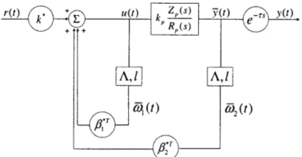
Figure 2-1: Exact model matching, Controller NC.

Under our assumptions, it follows [18] that there exists *,

0*/

ut(t) = + *Tc2(t) DT2(t) + k*r(t) (2.37) satisfies the exact model matching condition.

(t) k _(2.38)

r (t) m Rm (s)

Note that the model matching is achieved between the rational parts of the closed loop transfer function and of the reference model. On the other hand, it follows directly from (2.38) that

y(t)= - m e- T s

(2.39)

r(t) Rm(s)

which shows that the exact model matching condition is also satisfied between the total closed loop and the reference model transfer functions. Since 02(t) requires the output measurement at time t + 7, the control law given in (2.37) is non-causal. We refer to this closed loop system with the non-causal controller as "Controller NC" and it is depicted in Fig. 2-1.

It is also well known [18] that with zero initial conditions, there exists c, d e R" such that y(t) = cTI (t) + d+T' 2(t), which implies

Substituting (2.40) into (2.33) and rewriting (2.32) and (2.33) together in vector-matrix form, we get

C(t)

C

2(t)

A

LIc

I

and b =

A +

(

Substituting (2.42) into (2.37) we obtain that

u(t)

+ k*r(t),

which can equivalently be expressed as

= *TW(t) + a* (t) + T+ k*r(t).

+ k*r-(t).

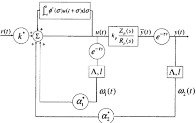
The controller (2.44) is causal and we refer to it as "Controller C". Defining

*

[P3(T P3 *T] and a* = [a*T aT], we get the following relationships between the

con-troller parameters of Concon-troller NC and Concon-troller C

a * = /P*eAT ¢*(a) = 3*e-AOb (2.45) (2.46)

E1

0J

Se-A"bu(t

a)

n*T

0-) du

u(t)

w2(t)

Figure 2-2: Exact model matching, Controller C.

The block diagram of Controller C is shown in Fig. 2-2.

In summary, an exact model matching controller, Controller C, can be designed for the time delay system (2.29) using a well known procedure for the delay free systems [18]. Note that the equivalence between Controller NC and Controller C shows that the latter relies on predicting the future output, y(t) to achieve exact model matching. This can be viewed as an equivalence result for higher order systems similar to that shown in Section 2.1 between (2.11) and (2.15).

Note that the model matching controller (2.44) was already introduced in [16] and [12]. The main contribution here is that we derive this controller by using the delay free part of the system dynamics, which considerably simplifies the design. In addition, instead of proposing a controller structure and proving that it is a model matching controller, we derive the controller using future state prediction which gives an insight about the controller structure. Finally, this derivation removes the assump-tion that the plant has poles with multiplicity one, which was assumed in the earlier papers. A similar result is given in [69] where it is stated that state prediction is a fundamental concept for time delay systems.

2.3.2

Adaptive Controller

The goal of this section is to design a model reference adaptive controller, motivated by the equivalence of the Controller NC and Controller C, for the plant described in (2.29) with unknown coefficients for the polynomials Zp(s) and Rp(s) and with unknown, positive high frequency gain kp. To start with, we assume that the relative

degree of the plant is one. The first step of the adaptive controller design is to design a fixed controller which satisfies the exact model matching with the reference model assuming that the plant parameters are known. This step was already completed in Section 2.3.1 resulting in the controller given in (2.44). In the second step, the controller parameters ac, a*, 0*(a) and k* are replaced by time-varying parameters

cal(t), a2(t), (t, ,) and k(t) and the goal is to determine the laws by which they are

adjusted so as to result in a stable system.

We define the following parameters:

0(t) - [(t) - k*, t ,(t) -0(t) - ,

d2(t) -f 2(t) - a2,

(t,

0)

¢(t, a) - 0*,

(t

+ k*r(t) +

f

(t)wi(t) + (t)w

+

k(t)r(t).

(2.47)

+

()

u(t) =

a

{

(t,

a)u(t

+ )d+

k(t)r(t)

Using the equivalence between (2.37) and (2.44), we can rewrite (2.47) as

U(t) = rCt) + dT (t)WI (t)

(t)

w

(t)

+ k r(t)

+ T(t)W2 (t) + (t, )u(t + a)da

+ k(t)r(t). (2.48)

(2.48) can then be represented as Xp(t) = AmXp(t) + bm[OT(t - T)Q(t - 7) + (t - T, c)u(t - T +

u)do

We showed in Section 2.3.1 that when the parameter errors are equal to zero, the closed loop transfer function is identical to that of the reference model. Therefore, the reference model can be described by the (3n)th order differential equation

Xm(t) = AmXm(t) + bmk*r(t - 7), ym(t) = hTXm(t) (2.51)

where,

Xm(t) ~ x w[ T *T₁T

hT (sI - Am)-1 bmk* = kmm. (2.52)

Rm

Note that x*(t), w (t) and w*(t) can be considered as the signals in the reference model corresponding to x,(t), wi(t) and w2(t) in the closed loop system. Therefore, subtracting (2.51) from (2.49), we get an error equation for the overall system as

+

(t- -7,

- 7 + a)d],

el(t)

where e(t) = X, - Xm and el (t) = y,(t) - ym(t).

The adaptive control law which guarantees convergence of the tracking error to zero and boundedness of all signals has the following form:

&(t) = --- el(t)w(t - )

0(t, a) = -7el (t)u(t - T + a), -T7 a < 0 (2.54)

where, y, and -y are positive, real adaptation gains.

When the relative degree n* equal to unity, it is easy to define a strictly positive real reference model Win(s). When n* = 2, an addition of an input ua to u as

Ua = 0. ' + (t, )u'(t + c)d,

2' =-aI' + ,

i = -au + u, a > 0

(2.55)

can be used to derive yet another error equation of the form

e(t) = Wm(S)(S + a)e- r [Or(t)Q(t) + ¢ (t, )u(t +

o-)dol

where a > 0 is chosen such that (s + a)Wm(s) is strictly positive real. Therefore it suffices to consider the stability of (2.53). The results can then be extended to the case when n* = 2 by making use of the additional input ua.

2.3.3

Stability Analysis

The following theorem confirms the desirable properties of the adaptive control law (2.54).

Theorem 2 Given initial conditions xp(0), u(n), 77 e [to - 27, to],

&C(),

[to - T,to], 37* s.t. V- e [0,7T*], the plant (2.29), the controller (2.47), and the

adaptive laws given by (2.54) have bounded solutions Vt >, 0 and limt, e (t) -o 0. We first state and prove the following lemma.

Lemma 1 Suppose a variable u(t) is of the form

0

u(t)

f(t) +

)(t

)u(t + o)d-

(2.57)

where u, f : [to-r, oo) -+ i, : [to, oo)x[-T, 0] --,+ and constants t',

cf,

R

f(t)

f,

02 (t, )da < c0, (2.58)

and

U2(t + )da = C2, Vt > ti. (2.59)

Then,

u(t') C 2(f + cco)eCo(t r- ,), Vt > t2. (2.60)

Proof of Lemma 1 Since (2.57) is an implicit integral equation, we derive in-equality (2.60) by considering a sequence u, and let u be the limit of this sequence as n -* co [70].

Define

uo(t) u(t ), 3t' < ti

Un+l (t / UV), t < ti)

S

(t', a)u,(t' + a)da + f(t'),

n = 0, 1..00

For t' > t' and n = 1, we have that

- uo(t;) =

f(t')

-T

f+

(f 0

(t

since the last parenthesis on the right hand side is being calculated over the time interval [t' - , t'j. Using (2.58) and (2.59), (2.63) can be rewritten as

u i(t;) - uo(t) ' + coc (2.64)

For t' > t' and n = 2 we have that

0 (t, a) (u1 t; +

f(f 2 ( ( t I) +

a) -

uo(t

0 - 0t 2

u)

uo(t;

+ u)

Using inequality (2.58) and a change of variables ( = t + a, (2.65) becomes

l2(t;)- l(tt;)

= CO U ( )- o(() 2 d( + UI(1() - o(()1

We know from (2.61) and (2.62) that ul(() - uo(() = 0 for

(

t'

can be further simplified as

t tI t 3> t,, (2.62) (2.63)

da)

IU'()

u

I(t)

C

I2(t')-

Ul(t')

2 U1 CO ul()

Substituting (2.64) into (2.67) we obtain that

0 ) 20 d) 1/2

- UO()1 2o _(2.67)

(2.68)

Continuing this procedure iteratively, we obtain that

S(f(c(t - t))n

1/ 2

4 f+ cico) ( - _n! -)

(2.69)

Note that the term (t' - t')"/n! in (2.69) is obtained due to successive integrations of (t'-t'). It can be shown using the ratio test [71] that

converges. This in turn implies that if S is defined as

o00

S = E (u n - Un-1)

n=1

the series

(j+

(

(2.70) it can be shown that

S - 2(f + clco)ec°(t"- t')

(2.71)

Please see Appendix A for a proof of (2.71).

Defining u - lim-,,, un, from (2.70) and (2.71), we obtain that

+ cco)e I

- C1Co)e o(t- )tO _(2.72)

This implies that,

(t,) < 2(f + cco)eco(t,-t') tj > ti (2.73)

and this completes the proof. Next, we describe the proof of Theorem 1.

Proof of Theorem 2 The proof is provided using the method of induction. Let

2(t;)- 1(t)

(f

Un+l (t) - Un(t')

the statement S be given by

S : IXp(

)I <

<

where U(.) is an analytic, bounded function of its arguments.

We note that Xp( ) and u(() is bounded for ( E [to - 2T, to). Using this fact, we complete the proof by showing that

I. S is true for k = 1.

II. If S is true for k, then it is true for k + 1

I and II allow us to conclude that all signals are bounded for all t > to. Finally, from Barbalat's Lemma, convergence of the error e to zero follows.

I. S is true for k = 1.

The proof of I is given in three steps, each of which starts with a brief summary.

Step 1. Some bounds on the signals are assumed in the time interval [to - 2r) and

the negative semi-definiteness of the Lyapunov functional time derivative in [to, to + 7) is shown, which yields the boundedness of the signals in [to, to + r). In addition, using Lemma 1, an upper bound for the control signal u(t) in [to, to + 7) is given.

Consider a Lyapunov Functional

V(t) = e(t)TPe(t) + O(t)To(t) + ¢(t, a)2dj

+

f

f

(

()d~dv

02

+ (, a)) daddv (2.75)

r +v -_

where P > 0. The error model (2.53) and the Lyapunov Functional (2.75) has been discussed in [19]. After algebraic manipulations, upper bound on the Lypaunov Function derivative can be computed as follows:

+

{

where

Q >

0 satisfies ATP + PAm =

-Q.

For the non-postiveness of 1(t), we need

to satisfy

Q-

0

0

(2.77)

Since w and u are dependent variables, condition (2.77) may not be easy to check.

Note however that the bound on V(t) is given by some bounds on w defined at

t-r

and

on u defined on the whole interval [t

-

2T, t

-

7]. It is shown below that this condition

can be replaced by bounds on signals w and u over the time interval [to

-

r, to] and

[to

- 2T,

to], respectively.

Suppose that

for some %i > 0, 2 > 0 and a r1 > 0 is such that

2T1 (Y1 + Y2) hmhT <

Q

Then, the following inequality is satisfied:

Q-2

--

V E [to, to + 7) ,VT e [0, rT]. (2.81)

It follows that V(t) is non-increasing for t E [to, to + 7). Thus, we have

V(to)

Xp,(1) to) + ||Xm()l| (2.82)

and hence,

Iw(

+

,V

to

(2.83)

2

0(() 2 <V(to),

(2.84)

( , )2do- ' V(to). (2.85)

To simplify the notation, we define

Io A max

(

(2.79), (2.84), (2.85) and (2.86), we obtain that

u(0)

2

(f

+

(

do

Io

V ( E [to, to + ) , (2.87)

where f depends only on Io. For simplicity, we will define g(72, Io, T) - 2

(f

and rewrite (2.87) as

u()I

g(7-,

7)

Step 2. A delay value is found that leads to a non-increasing V over [to, to +

2T],

which in turn shows that Xp is bounded over the same interval.

27-2 (I4 + (max(y2, 9('2, I0, T2)))2 72) hmhTm

< Q.

For

r

Therefore, we obtain that

lXp,(()

1 o, V4 E [to, to + 27) .

(2.90)

Step 3. It is shown that the bound on the control signal u over the time interval

[to, to + 7) depends only on A,, bp, T, Io and _{T. The proof given in this section is}

similar to the one given in [72], Lemma 5. Let Iu = {tI lu(t)l = supst lu(a)l}.

Let [t, - 7, t, - 7 + T] c Tu c [to, to + 7). Defining z(t) = u(t - 7), we can solve (2.31) as

Xp(ti + T) = xp(ti)eApT + eAp(T+t,-t)bpz(t)dt (2.91)

Positive constants c6 and c7 exists such that I eApTl < C6 and II ST eAP"bpda I > C7

and

Ilx,(t,

+

T)II >

Ic

z(t,)l - c6

Ijx(t|)Iil

(2.92)

Note that we obtain (2.92) by selecting T such that the terms of the vector eApabp does not change sign for a e [0, T]. In addition, note that once T is selected properly, the inequality (2.92) is satisfied for any time interval [t3, tj + T] as soon as [tj - 7, t, +

T - 7] c Tu c [to, to + 7) since the constants c6 and c7 are determined only by the

size of T.

From (2.92) we obtain that

IlXp(t

+

T)II

+ JIx,(t)ll

>

Iz(ti)l

(2.93)

or