HAL Id: hal-02326771
https://hal.archives-ouvertes.fr/hal-02326771
Submitted on 15 Dec 2020HAL is a multi-disciplinary open access archive for the deposit and dissemination of sci-entific research documents, whether they are pub-lished or not. The documents may come from teaching and research institutions in France or abroad, or from public or private research centers.
L’archive ouverte pluridisciplinaire HAL, est destinée au dépôt et à la diffusion de documents scientifiques de niveau recherche, publiés ou non, émanant des établissements d’enseignement et de recherche français ou étrangers, des laboratoires publics ou privés.
Imaging rapid early afterslip of the 2016 Pedernales
earthquake, Ecuador
Louisa L.H. Tsang, Mathilde Vergnolle, Cedric Twardzik, Anthony Sladen,
Jean-Mathieu Nocquet, Frédérique Rolandone, Hans Agurto-Detzel, Olivier
Cavalié, Paul Jarrin, Patricia Mothes
To cite this version:
Louisa L.H. Tsang, Mathilde Vergnolle, Cedric Twardzik, Anthony Sladen, Jean-Mathieu Nocquet, et al.. Imaging rapid early afterslip of the 2016 Pedernales earthquake, Ecuador. Earth and Planetary Science Letters, Elsevier, 2019, 524, pp.115724. �10.1016/j.epsl.2019.115724�. �hal-02326771�
1 | P a g e
Imaging rapid early afterslip of the 2016 Pedernales earthquake,
1
Ecuador
2 3
Louisa L.H. Tsang1, Mathilde Vergnolle1, Cedric Twardzik1, Anthony Sladen1, Jean-4
Mathieu Nocquet1,2, Frédérique Rolandone3, Hans Agurto-Detzel1, Olivier 5
Cavalié1,4, Paul Jarrin1,3, Patricia Mothes5 6
1. Université Côte d’Azur, CNRS, Observatoire de la Côte d’Azur, IRD, Géoazur, Campus 7
CNRS, 250 rue Albert Einstein, Sophia Antipolis 06560 Valbonne, France. 8
2. Université de Paris, UMR 7154 CNRS, Paris, France. 9
3. Sorbonne Université, CNRS-INSU, Institut des Sciences de la Terre Paris, ISTeP UMR 7193, 10
F-75005, Paris, France. 11
4. Université de Lyon, UCBL, CNRS, LBL-TPE, 69622 Villeurbanne, France. 12
5. Instituto Geofísico, Escuela Politécnica Nacional, 2759 Quito, Ecuador. 13
Corresponding author:
14
Louisa L.H. Tsang. louisa.tsang@geoazur.unice.fr
15
Present address:
16
Géoazur, Campus CNRS, 250 rue Albert Einstein, Sophia Antipolis 06560 Valbonne, France. 17
2 | P a g e
Abstract
19
High-Rate (HR) GPS time series following the 2016 Mw 7.8 Pedernales earthquake suggest 20
significant postseismic deformation occurring in the early postseismic period (i.e. first few hours 21
after the earthquake) that is not captured in daily GPS time series. To understand the 22
characteristics of early postseismic deformation, and its relationship with the mainshock 23
rupture area, aftershocks and longer-term postseismic deformation, we estimate the spatio-24
temporal distribution of early afterslip with HR-GPS time series that span ~ 2.5 minutes to 72 25
hours after the earthquake, and compare with afterslip models estimated with daily GPS time 26
series spanning a similar postseismic time period and up to 30 days after the earthquake. Our 27
inversion technique enables us to image the nucleation of afterslip in the initial hours after the 28
earthquake, bringing us closer to the transition between the coseismic and postseismic phases. 29
The spatial signature of early afterslip in the region updip of the mainshock rupture area is 30
consistent with longer-term afterslip that occurs in the 30-day postseismic period, indicating 31
that afterslip nucleated updip of and adjacent to peak coseismic slip asperities, in two localized 32
areas, and subsequently continued to grow in amplitude with time in these specific areas. A 33
striking difference, however, is that inversion of the 72-hour HR-GPS time series suggests early 34
afterslip within the mainshock rupture area, but which may have been short-lived. More 35
interestingly, we find that postseismic slip starts immediately after the earthquake at a rapid 36
rate. Indeed, we find that early afterslip represents a significant contribution to the postseismic 37
geodetic moment – afterslip in the first 72 hours is ~60 % greater than that estimated with daily 38
GPS time series that span the first three post-earthquake daily GPS positions (i.e. covering the 39
same time window). The results of our study demonstrate that imaging the spatio-temporal 40
evolution of afterslip using subdaily GPS time series is important for evaluating postseismic slip 41
3 | P a g e
budgets, and provides additional insights into the postseismic slip behaviour of faults. 42
Keywords: afterslip; postseismic; subduction; Ecuador; aftershocks; GPS
4 | P a g e
1. Introduction
44
Afterslip plays an important role in redistributing stresses on and around megathrusts following 45
subduction zone earthquakes, and can represent a significant amount of moment release [e.g. 46
Hsu et al., 2006]. Thus, mapping out at various timescales where it occurs is vital for assessing 47
seismic hazard on neighbouring sections of megathrusts. Most afterslip imaging studies are 48
conducted using daily GPS time series spanning timescales ranging from weeks to years 49
following the earthquake [e.g. Hsu et al., 2006; Tsang et al., 2016]. The first data point in these 50
postseismic time series is at best taken on the first, or the second day, after the earthquake. 51
However, these postseismic daily GPS time series do not enable us to understand the nature of 52
postseismic deformation occurring in the minutes to hours following the earthquake, hereafter 53
referred to as the early postseismic period. Rather, early postseismic deformation is commonly 54
captured within the static coseismic offset calculated with InSAR or daily GPS time series 55
spanning a certain number of days before and after the earthquake. This manner of calculation 56
can result in a contamination of the coseismic signal by early postseismic deformation, resulting 57
in potential biases in the estimated coseismic source model. This likely explains why seismic 58
moments for the same earthquake estimated from only daily GPS measurements can range 59
from 1.5 to 2 times higher than those using only seismic data [e.g. Langbein et al., 2006]. 60
Furthermore, daily GPS time series do not allow us to resolve the transition between the 61
coseismic and postseismic phases of deformation, and can hence potentially result in erroneous 62
estimates of coseismic and postseismic slip budgets on faults. Thus, better understanding the 63
early phase of postseismic deformation requires analysis of high-rate GNSS position time series 64
that can capture the associated signal on the Earth’s surface. 65
5 | P a g e
Thus far, only a handful of studies have focused on the early postseismic period. These studies 67
focus on the 2004 Mw 6.0 Parkfield earthquake in California [Langbein et al., 2006], 2003 Mw 8.0 68
Tokachi-Oki [Miyazaki and Larson, 2008; Fukuda et al., 2009] and 2011 Mw 9.1 Tohoku-oki 69
earthquakes [Munekane, 2013] in Japan, 2012 Mw 7.6 Nicoya earthquake in Costa Rica 70
[Malservisi et al., 2012], and the 2010 Mw 8.8 Maule, 2014 Mw 8.3 Illapel and 2016 Mw 7.8 71
Pedernales earthquakes in South America [Twardzik et al., 2019]. By analyzing HR-GPS position 72
time series following these earthquakes, these studies demonstrate that the magnitude of early 73
postseismic deformation is significant. For example, the geodetic moment in the early 74
postseismic period following the 2012 Nicoya earthquake represents ~57 % of that released 75
during the first 70 days [Malservisi et al., 2012]. Malservisi et al. [2012] and Munekane [2013] 76
estimated snapshots of the spatial distribution of early afterslip by inverting cumulative offsets 77
calculated with a certain length time window of HR-GPS time series. However, this approach 78
does not enable us to ensure coherency of afterslip from one time step to another. Also, it 79
should be noted that cumulative offsets calculated with HR-GPS time series can vary depending 80
on the level of noise in the time series and the method used to calculate these offsets. Of the 81
studies mentioned above, only Miyazaki and Larson [2008] inverted HR-GPS time series 82
(spanning 4 hours after 2003 Tokachi-oki earthquake) to image the spatio-temporal evolution of 83
afterslip. Their results show a complex evolution of early afterslip and suggest that it might have 84
triggered the aftershock that occurred ~1.2 hours after the mainshock. They concluded that 85
depth-dependent properties on the fault influence the propagation patterns of afterslip seen in 86
their models. Fukuda et al. [2009] investigated postseismic time series of this earthquake too, 87
with a focus on the sudden acceleration of motions ~1.2 hours after the earthquake. They 88
argue that the timing of this acceleration phase is driven by stress changes from the mainshock 89
6 | P a g e
and the frictional parameters of the rate-and-state friction law, rather than due to the timing of 90
the aftershock. Their results support theoretical studies demonstrating that faults experience 91
an initial acceleration phase of afterslip, which is then followed by decelerating afterslip 92
governed by steady-state velocity-strengthening friction [Perfettini and Ampuero, 2008]. 93
Clearly, investigating the spatio-temporal evolution of early postseismic deformation is relevant 94
for understanding the physical mechanisms driving fault slip behaviour, as well as resolving its 95
relationship with the mainshock rupture area, ensuing aftershocks, longer-term postseismic 96
deformation, and quantifying its contribution to the postseismic slip budget. 97
98
Here, we model HR-GPS postseismic time series to estimate the spatio-temporal evolution of 99
early afterslip following the 2016 Mw 7.8 Pedernales earthquake (16 April 2016, 23:58:33) in 100
Ecuador (Figure 1). The Ecuadorian megathrust hosts a diverse range of seismic and aseismic 101
behaviour that has been studied in detail with regional GPS and seismic networks, as well as 102
marine seismic studies [e.g., Collot et al., 2017; Font et al., 2013; Vallée et al., 2013; Mothes et 103
al., 2013; Chlieh et al., 2014; Nocquet et al., 2014; 2016; Marcaillou et al., 2016; Rolandone et 104
al., 2018; Gombert et al., 2018; Vaca et al., 2018; Segovia et al., 2018; Agurto-Detzel et al. 105
(submitted); Twardzik et al., 2019]. The optimal location of these networks have enabled 106
detection of a number of slow slip events, repeating earthquakes and seismic swarms, as well as 107
significant afterslip in the month following the Pedernales earthquake [Vallée et al., 2013; 108
Rolandone et al., 2018; Vaca et al., 2018; Segovia et al., 2018]. These findings indicate that 109
aseismic slip processes represent a significant mode of strain release along the megathrust, and 110
it is therefore important to understand their contribution to megathrust slip budgets. 111
7 | P a g e
In this study, we capitalize on the availability of rich postseismic geodetic datasets from 113
Twardzik et al. [2019] and Rolandone et al. [2018] to image the spatio-temporal distribution of 114
early afterslip in the first 72 hours after the earthquake, and compare this to afterslip estimated 115
with daily GPS time series spanning the same time period (i.e. the first three post-earthquake 116
daily GPS positions), as well as spanning the longer, 30-day post-earthquake time period (Figure 117
2). We also examine relationships between early afterslip, the earthquake rupture area, and the 118
spatio-temporal distribution of relocated aftershocks. 119
8 | P a g e
2. Data
120
We use GPS data from 27 stations of the Ecuadorian continuous GPS network that were 121
installed before the earthquake, and from which both HR-GPS and daily GPS time series were 122
available (Figure 3). The horizontal components of the daily GPS time series from these stations 123
were processed by Rolandone et al. [2018], with positions expressed with respect to the first 124
daily GPS position (the day after the earthquake). In the days following the earthquake, 4 Mw> 6 125
aftershocks occurred in the region updip of the mainshock rupture area. Coseismic offsets (and 126
likely some ensuing postseismic deformation) associated with these aftershocks are visible in 127
the time series of stations CABP and MOMP on the 22 and 20 April, respectively (Figure S1). 128
We did not attempt to correct the time series for these offsets, due to the absence of a 129
technique to reliably estimate and remove the coseismic and postseismic signals associated with 130
these aftershocks. No visible offsets associated with these aftershocks are observed at other 131
stations. 132
133
The 30-second HR-GPS time series from these stations were processed by Twardzik et al. 134
[2019]. The time series span ~72 hours after the earthquake from 17 April 2016, 00:02:00 to 135
19 April 2016, 23:59:59. The first position in the HR-GPS time series was chosen to ensure that 136
the time series are not contaminated by seismic waves associated with the mainshock (see 137
Twardzik et al. [2019] for details). We downsampled these time series to a position every 60 138
seconds, and used only the horizontal component of displacements, as the vertical component 139
of displacements have relatively low signal-to-noise ratios and large uncertainties. 140
9 | P a g e
We examined the gCMT catalog of regional earthquakes, and found no significant signals of 142
these earthquakes in the HR-GPS time series. The largest 72-hour cumulative displacements are 143
observed at stations nearest the mainshock rupture area (Figure 3): MOMP, CABP and PDNS, 144
with values of 5.5, 4.6 and 3.3 cm, respectively. The 30-day cumulative displacements for these 145
stations, calculated from the daily GPS time series, are 12.6, 11 and 7.2 cm, respectively. 146
147
The 60-second HR-GPS time series are relatively noisy (Figures S2, S3). Hence, to verify that 148
our inversion results are not significantly influenced by noise in the time series, we performed 149
four additional inversions with time series low-pass filtered at various cut-off frequencies, to 150
extract the reliable features of the models (Text S1, Figure S3) (see next section for details). 151
10 | P a g e
3. Inversion method to estimate the spatio-temporal distribution of afterslip
152
We assume that the signal in the early postseismic time series represents predominantly 153
afterslip on the megathrust. This approximation seems valid considering that postseismic signals 154
are recorded at stations covering a region greater than would be expected from poroelastic 155
effects, the latter of which are likely to occur in more localized regions [e.g. Tung and 156
Masterlark, 2018]. Also, the early postseismic time period considered is shorter than 157
characteristic relaxation times associated with typical mantle viscosities previously reported at 158
subduction zones (assuming a linear mantle rheology, mantle viscosities of 1017 to 5*1019 Pa s 159
correspond to relaxation times ranging from ~38 days to 50 years). Even so, we do not exclude 160
the possibility that our modelling approach might represent deformation associated with other 161
postseismic mechanisms mapped onto the fault. We estimated the spatio-temporal distribution 162
of afterslip that span the first: (1) 72 hours (with HR-GPS time series), (2) 2 days (with time 163
series of the first three daily GPS positions), and (3) 30 days (with daily GPS time series) (Figure 164
2). While Rolandone et al. [2018] already published a spatio-temporal 30-day afterslip model, 165
we estimated the spatio-temporal 2-day and 30-day models using the same inversion strategy as 166
that used to estimate the 72-hour model, in order to enable a fair comparison between them. 167
168
Since the HR-GPS time series are relatively noisy compared to daily GPS time series, a method 169
is required to filter for the main postseismic signal in the presence of considerable noise in the 170
time series. We adopted the Principal Component Analysis-based Inversion Method (PCAIM) 171
[Kositsky and Avouac, 2010] to invert for the spatio-temporal distribution of afterslip, as this 172
method allows the main postseismic signal to be represented with a small number of principal 173
components. The surface displacement patterns associated with each principal component are 174
11 | P a g e
inverted to obtain a principal slip distribution; these are then linearly combined together with 175
the corresponding time functions to obtain a model of the spatio-temporal evolution of afterslip 176
(Text S2). While PCAIM has been validated on standard daily GPS time series, to the best of 177
our knowledge it has never been implemented yet with noisy HR-GPS time series. However, it 178
has been shown to be effective in estimating afterslip with noisy daily GPS time series [e.g. 179
Gualandi et al., 2014]. To determine the optimum number of principal components to 180
represent the postseismic signal, we analysed the time series fits as incrementally more 181
principal components were employed, examined the time functions, surface displacement 182
patterns associated with each principal component, and the corresponding principal slip 183
patterns. 184
185
For the HR-GPS time series, we found that one principal component adequately represents the 186
postseismic signal (Text S2, Figure S4), while for the daily GPS time series, two principal 187
components were required (Figure S5). The additional component for the latter case is 188
probably due to the presence of a slow slip event in the daily GPS time series (discussed in 189
section 5.6). Offsets in the daily GPS time series seen at stations CABP and MOMP mentioned 190
previously are not present in the time functions of the first two principal components, when 191
the data are decomposed. Therefore, inclusion of these offsets does not significantly influence 192
the afterslip model results. 193
194
We estimated afterslip on the same fault interface geometry employed by Rolandone et al. 195
[2018]. This fault geometry spans latitudes ~2°S to ~1°N, extends to a depth of 80 km, and 196
follows the SLAB1.0 model along this section of the Andean megathrust [Hayes et al., 2012]. 197
12 | P a g e
The fault interface was discretized into quasi-equilateral triangles with 10-km-long edges. The 198
horizontal displacements at each GPS station due to slip on each sub-fault patch were calculated 199
with Okada’s solutions for deformation due to point dislocations embedded in a homogeneous 200
elastic half-space [Okada, 1992]. Similar to the approach of Rolandone et al. [2018], the rake 201
angle on each triangular patch was fixed to a direction that is consistent with the Nazca/North 202
Andean block relative velocity determined by Nocquet et al. [2014] (although we note that 203
allowing the rake angle to vary by +/- 45° from 90° does not significantly affect the results; 204
Figure S6). Positivity constraints were applied to ensure trench-directed slip. 205
206
The Laplacian constraints, which control the degree that slip is smoothed across neighbouring 207
patches, were weighted spatially based on the sensitivity of each station to slip on each sub-fault 208
patch (following the method of Ortega-Culaciati [2013]). The spatial variation of this weighting 209
results in more smoothing of slip in poorly resolved areas (Text S3, Figure S7). In addition, λ, 210
the value controlling the strength of the Laplacian constraints, was selected for each model 211
based on the standard L-curve analysis [Hansen, 1992], corroborated by visual examination of 212
the slip distributions associated with each value of λ. The optimum value of λ represents the 213
best trade-off between the data-model misfits and the model norm, and which preserves the 214
key spatial characteristics of the solution (Text S3, Figure S8). We note that the optimum value 215
of λ differs by three orders of magnitude between the case of inverting the HR-GPS and the 216
daily GPS time series, because in the case of the daily GPS time series, we took into account 217
the data uncertainties (although we retrieve a similar spatial distribution of slip even if we do 218
not take into account the data uncertainties). On the other hand, we did not take into account 219
the uncertainties of the HR-GPS data in the inversion, as these could not be reliably estimated. 220
13 | P a g e
221
As mentioned in the previous section, for the 72-hour dataset, we performed five inversions, 222
with each inversion using time series with various degrees of filtering applied, in order to 223
extract the reliable features of afterslip. Our reference model is the afterslip distribution 224
estimated with time series filtered with a cut-off frequency corresponding to a time period of 225
~2.7 hours, chosen as it yields visually smooth time series (Text S1). 226
14 | P a g e
4. Results
227
4.1. Early afterslip distribution from the 72-hour dataset
228
Six main early afterslip areas are evident in all five models (Areas A-F, Figure 3, inset, and Figure 229
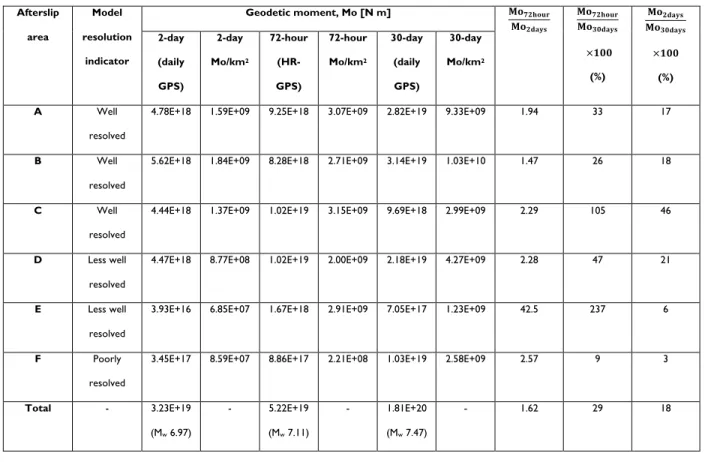
S9). The five models indicate geodetic moments ranging from 5.16E+19 to 6.35E+19 N m (Mw 230
7.11-7.17), assuming a rigidity of 30 GPa (Table S1). 231
232
Our reference model, shown in Figure 3, yields a reduced chi-square of 0.65. Assuming a 233
rigidity of 30 GPa, the estimated total geodetic moment is 5.22E+19 N m, which is equivalent to 234
a moment magnitude of Mw 7.11. This moment estimate is ~9.7% of the coseismic moment as 235
estimated by Nocquet et al. [2016]. The model shows peak cumulative afterslip of ~ 30 cm 236
concentrated in two areas updip of and adjacent to asperities that experienced the largest 237
coseismic slip (Areas A and B). The largest cumulative geodetic moment occurred in area A 238
(9.25E+18 N m; Mw 6.61), while less occurred in area B (8.28E+18 N m; Mw 6.58). In addition, 239
~13-18 cm of cumulative afterslip is concentrated within the southern portion of the mainshock 240
rupture area (area C) and immediately downdip of the mainshock rupture area (area D), with 241
each area amounting to an estimated geodetic moment of 1.02E+19 N m (Mw 6.63). ~1.67E+18 242
N m (Mw 6.12) of geodetic moment is estimated north of the mainshock rupture area (area E). 243
244
Further south-east, ~190 km from the Pedernales earthquake hypocentre, ~ 28 cm of 245
cumulative slip is estimated on a single patch located north of La Plata Island (area F, Figure 3). 246
This patch of slip is located close to the remotely triggered slow slip event that was reported 247
by Rolandone et al. [2018]; we discuss these results in section 5.6. 248
15 | P a g e
While we demonstrate that the main afterslip areas shown in Figure 3 (inset) are reliable based 250
on inverting various groups of filtered time series, we additionally conducted synthetic tests (in 251
the next section) to assess the resolution of slip in our reference model, which is related to the 252
fault geometry that we employed and the spatial distribution of GPS stations. 253
16 | P a g e
4.2. Model resolution
254
For each main afterslip area, 1 m of trench-perpendicular slip was assigned to each sub-fault 255
patch. Then, horizontal displacements at each station were calculated with the Okada model 256
[Okada, 1992]. Synthetic time series at each station were subsequently calculated by multiplying 257
the horizontal displacements with the synthetic normalized time function (based on the first 258
principal component obtained from decomposition of the 30-day GPS time series). For each 259
station, noise was added to the synthetic time series that is on the order of the average 260
standard deviation from the mean position estimated using the pre-earthquake HR-GPS time 261
series (Figure S2). For the inversion, we employed the same value of λ as that in our reference 262
model. 263
264
The magnitude of peak slip is well recovered in the two areas updip of the mainshock rupture 265
area (Figure 4a), as well as within the mainshock rupture area (Figure 4b), as the inversion 266
indicates that ~ 73-78 % of the input synthetic slip is recovered. On the other hand, the 267
magnitude of peak slip is not well recovered downdip of the mainshock rupture area (Figure 268
4c), and near Esmeraldas (Figure 4d), with only ~ 30-38 % of the input synthetic slip recovered 269
in the inversion, and significant smoothing of slip across adjacent sub-fault patches. These 270
conclusions are supported by the recovered slip model based on an input model where all main 271
afterslip areas were assigned trench-perpendicular synthetic slip of 1 m (Figure 4e); slip in the 272
updip regions is well recovered, while slip downdip and near Esmeraldas is not. In the 273
mainshock rupture area, slip is recovered, but is smeared across neighbouring sub-fault patches. 274
Importantly, Figure 4a demonstrates that slip in the southern updip area is not smeared into the 275
mainshock rupture area, suggesting that slip in area C (Figure 3) is not an artifact of the spatial 276
17 | P a g e
smoothing that we employ. In addition, slip in area C is evident in rougher afterslip models from 277
all five inversions (Figure S8), suggesting that this is a reliable feature, since it is evident 278
regardless of the temporal smoothing of the time series and spatial smoothing of slip. 279
280
We present in Text S4 and Figure S11 results of implementing an alternative method of 281
assessing the resolution of our model. The results substantiate our conclusions drawn here. 282
Furthermore, Rolandone et al. [2018] reported that slip areas of > 40 km on this fault 283
geometry are well resolved. 284
18 | P a g e
5. Discussion
285
5.1. Comparison of 72-hour and 2-day afterslip models highlights the
286
significant contribution of early afterslip
287
Figure 5 and Table 1 show that in each of the six main afterslip areas, the geodetic moment of 288
afterslip in the 72-hour model is greater than that in the 2-day model. The 72-hour model 289
suggests afterslip in two areas that are not visually evident in the 2-day model: north of the 290
mainshock rupture area near Esmeraldas and north of La Plata Island (areas E and F, 291
respectively, Figure 5c), where the difference in geodetic moment is a factor of ~43 and 2.6, 292
respectively. However, our model resolution tests suggest that slip is not well resolved in these 293
two areas. In other areas (areas A-D), the geodetic moment between the two models differs by 294
a factor of ~1.5 to 2.3. These findings suggest enhanced afterslip in these areas during the first 295
12 hours, the period that is not captured by the daily GPS time series. 296
297
South of the mainshock rupture area (area G, Figure 5c), more afterslip is estimated in the 2-298
day model. According to our approach of extracting the robust features of the 72-hour model 299
based on various filtered time series (Figure S9), slip here is not a reliable feature and may be 300
due to high frequency noise in the time series. Slip here in the 72-hour model is thus not 301
accurately resolved. 302
303
Overall, the estimated geodetic moment of the 72-hour model is a factor of ~1.6 greater than 304
that of the 2-day model (Table 1) (this factor is ~1.68 in the case of excluding poorly resolved 305
slip areas), suggesting that not accounting for the postseismic deformation recorded 306
immediately after the coseismic phase could result in an underestimation of the postseismic 307
19 | P a g e
geodetic moment by ~60 % - very early afterslip (i.e. before the first GPS daily position) 308
therefore contributes significantly to the postseismic geodetic moment. 309
310
Our 72-hour afterslip model explains why coseismic slip distributions estimated with InSAR 311
data place coseismic slip near the trench. For example, from InSAR data that span 6 days after 312
the earthquake, He et al. [2017] found coseismic slip that extends to regions near the trench, 313
and a higher estimated seismic moment compared with studies that either exclude or put a low 314
weighting on InSAR data [e.g. Nocquet et al., 2016; Ye et al., 2016]. As the InSAR data likely 315
contain deformation due to both the coseismic and early postseismic slip, their models are 316
consistent with our results showing early afterslip located updip of the mainshock rupture area. 317
20 | P a g e
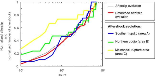
5.2. Spatio-temporal evolution of afterslip and aftershocks in the first 72 hours
318
Figure 6 shows how afterslip evolves in time within the 72-hour period. As pointed out by 319
Rolandone et al. [2018], the spatial distribution of shallow afterslip shows little correspondence 320
to that of stress changes induced by coseismic slip. Interestingly, our results suggest that this 321
spatial distribution, where slip is localized in a few specific areas rather than broadly updip and 322
downdip of the rupture area, is in place immediately after the earthquake. In the subsequent 72-323
hour postseismic period, the spatial distribution of afterslip remains fixed, with the amplitude of 324
afterslip increasing with time. This latter finding is expected given that only one principal 325
component was used (and is sufficient) to represent the postseismic time series, such that the 326
slip evolution on each patch is governed by the same time function. This specificity of using one 327
principal component also limits our capability to discern possible patterns of accelerating 328
afterslip in the different afterslip areas. Importantly, our spatio-temporal modelling approach 329
enables us to analyze an enriched picture of the temporal evolution of afterslip that indicates 330
that the highlighted updip areas are particularly prone to host afterslip, and enables us to 331
compare our results with the spatio-temporal evolution of aftershocks. 332
333
Aftershocks occur due to the release of static and/or dynamic stress changes associated with 334
the mainshock [Dieterich, 1994; Felzer and Brodsky, 2006; Stein, 1999]. In addition, a number 335
of studies have reported similar temporal evolution of afterslip and aftershocks following large 336
earthquakes, which support a model whereby aftershocks are produced when rate-weakening 337
asperities are loaded by afterslip and driven to coseismic failure [e.g. Hsu et al., 2006; Perfettini 338
and Avouac, 2004]. To explore the spatio-temporal relationship between afterslip and 339
aftershocks in the first 72 hours, we analyzed the aftershock catalogue of Agurto-Detzel et al. 340
21 | P a g e
(submitted). Errors in the aftershock locations at the 68 % confidence level are ~12 and 13 km 341
in the horizontal and vertical directions, respectively. Based on their one-year-long aftershock 342
catalogue, Agurto-Detzel et al. (submitted) reported a threshold magnitude of completeness of 343
2.5. However, the catalogue is most likely incomplete in the initial hours after the earthquake, 344
as during this period the noise level is higher and events are harder to identify. To be more 345
conservative, we therefore analyzed ML ≥ 3.5 aftershocks in this study (Figure S12). 346
347
Figure 6 shows that relocated M3.5+ aftershocks appear to concentrate in regions bordering 348
the two updip peak afterslip areas (A and B), which is consistent with the results from other 349
studies that reported limited occurrence of aftershocks within the regions of peak afterslip [e.g. 350
Hobbs et al., 2017; Hsu et al., 2006]. In area A, the aftershock-afterslip moment ratio, 351
expressed as a percentage of the cumulative aftershock seismic moment to the cumulative 352
afterslip geodetic moment, is 11%, while in area B, this ratio is ~ 6% (seismicity in each area is 353
defined using the limits shown in Figure S12). These ratios indicate that the majority of the 354
postseismic deformation is aseismic. A large number of aftershocks are also located within the 355
mainshock rupture area; these occur in the region between the two peak coseismic slip 356
asperities, and border the patches of peak afterslip in area C. However, the cumulative seismic 357
moment released in area C is small - the aftershock-afterslip moment ratio is 0.93 %; around an 358
order of magnitude smaller than in the two updip afterslip regions. In contrast, there is sparse 359
seismicity in the region downdip of the mainshock. 360
361
In the first 72 hours, the similarity in the temporal evolution of afterslip and numbers of ML> 362
3.5 aftershocks in the two updip areas (A and B) (Figure 7) suggests that aftershocks in these 363
22 | P a g e
regions are likely driven by afterslip, consistent with the findings of Agurto-Detzel et al. 364
(submitted) based on their one-year-long catalogue. In contrast, the evolution curves suggest 365
that in area C, there is a much larger fraction of aftershock occurrence in the first ~48 hours 366
compared to other areas (Figure 7). We hypothesize that a proportion of aftershocks 367
represent the release of residual coseismically-induced stress on the megathrust interface as 368
well as in the overlying crust (Figure S12), and are thus possibly controlled by two different 369
processes. In addition, though our analysis may be limited by the completeness of the 370
aftershock catalogue in the first 72 hours, the evolution curves (note that Figure 7 is in semi-371
logarithmic scale) suggest that early afterslip and aftershocks do not appear to follow an Omori-372
type law, in contrast to findings from analyzing aftershocks over a longer time period of ~1 year 373
[Agurto-Detzel et al. (submitted)]. 374
375
Interestingly, the 1942 earthquake has been inferred to have roughly the same rupture area as 376
the 2016 earthquake [Ye et al., 2016; Nocquet et al., 2016], and aftershocks following the 1942 377
earthquake were mainly located seaward of the hypocentre [Mendoza and Dewey, 1984], 378
implying that these aftershocks may have been driven by afterslip updip of the mainshock 379
rupture area too. If so, these observations may indicate that aseismic slip behaviour, and by 380
inference, frictional properties, persist through at least two seismic cycles. 381
23 | P a g e
5.3. 30-day afterslip distribution from daily GPS time series
382
Our 30-day afterslip results (Figure 8b) are consistent with that estimated by Rolandone et al. 383
[2018] (data-model fits at representative stations are shown in Figure 8d; the spatio-temporal 384
evolution of afterslip in the first 30 days and data-model time series fits at all stations are shown 385
in Figures S13 and S14, respectively). Estimated afterslip in the first 30 days amounts to a 386
geodetic moment of 1.71E+20 N m, equivalent to an ~Mw 7.46. In the region updip of the 387
mainshock rupture area, the spatial distribution of 30-day afterslip is consistent with that in the 388
first 72 hours, indicating that afterslip nucleated in localized areas updip of and adjacent to 389
patches that experienced the largest coseismic slip, and subsequently continued to grow in 390
amplitude with time. Similar to the case within the first 72 hours, aftershocks in the subsequent 391
28 days mostly surround the updip afterslip areas (Figure 8b). Peak afterslip is concentrated in 392
area B (~70 cm) and might have extended to the trench, though the model resolution is poor 393
close to the trench. In both areas A and B, estimated afterslip in the first 72 hours is ~30 % of 394
that accumulated in the first 30 days (Table 1). 395
396
On the other hand, there are differences between the 72-hour and 30-day afterslip models 397
within, downdip and north of the mainshock rupture area (areas C, D and E, respectively). In 398
area E, we have already pointed out that resolution of slip here in the 72-hour model is poor 399
(see section 4.2). In area C, where slip is better resolved, a greater amount of afterslip likely 400
occurred in the first 72 hours, but this afterslip may have been short-lived, as limited afterslip is 401
imaged in these areas in the 30-day model. Also, notwithstanding the poorer model resolution 402
in the downdip region, a comparison of the two models shows that afterslip here nucleated in 403
24 | P a g e
the first 72 hours immediately downdip of the mainshock rupture at ~ 30-50 km depths, and 404
may have subsequently migrated southwards and extended to ~40-70 km depths. 405
25 | P a g e
5.4. Spatial overlap of early afterslip with the mainshock rupture area
406
Comparison of our 72-hour, 2-day and 30-day models suggests that afterslip in the mainshock 407
rupture zone rapidly decayed with time, likely within the first 12 hours after the earthquake. 408
There is a spectrum of observations concerning afterslip occurring in mainshock rupture zones. 409
Some studies have reported observations of coseismic deformation that is anticorrelated with 410
afterslip and/or aftershock areas [e.g. Perfettini et al., 2010; Sladen et al., 2010]. These studies 411
support the ‘rate-state asperity model’ that stipulates that velocity-weakening patches on the 412
fault that host seismic ruptures do not manifest significant afterslip. On the other hand, a 413
number of recent studies report that afterslip in coseismic rupture zones is needed to explain 414
geodetic observations, challenging this conceptual model [e.g. Barnhart et al., 2016; Bedford et 415
al., 2013; Miyazaki and Larson, 2008; Johnson et al., 2012; Salman et al., 2017]. It is possible that 416
some of these observations can be explained by modelling biases. For example, coseismic slip 417
distributions estimated with InSAR data often span the early and longer postseismic period, 418
which potentially results in some amount of postseismic deformation being mapped as 419
coseismic slip. Another bias may lie in the choice of model smoothing parameters for 420
postseismic slip models [e.g. Fukuda et al., 2009]. 421
422
Despite these biases, several physical mechanisms have been proposed to explain the overlap of 423
afterslip and coseismic slip areas. Helmstetter and Shaw [2009] stipulate that frictional 424
properties on the megathrust are not steady state. Physical processes such as dynamic 425
weakening and rupture directivity may push normally velocity-strengthening patches to 426
participate in coseismic ruptures [e.g. Noda and Lapusta, 2013, Salman et al. 2017]. Along the 427
Ecuadorian subduction zone, Kanamori and McNally [1982] proposed a model in which distinct 428
26 | P a g e
‘asperities’ of the 1942, 1958 and 1979 ruptures are separated by weak zones that typically 429
behave aseismically, but can slip abruptly when driven by failure of neighbouring asperities - this 430
mechanism was proposed to explain the coordinated rupture of all three asperities in a Mw 8.8 431
earthquake in 1906. Indeed, frictional properties may vary during the course of the earthquake 432
cycle, and patches that are conditionally stable may participate in both coseismic and aseismic 433
slip phases. Yabe and Ide [2018] modeled a frictionally heterogeneous fault system and their 434
quasi-dynamic numerical simulation results were able to reproduce afterslip and aftershocks 435
occurring around and within the mainshock rupture zone. They proposed that if patches within 436
the mainshock rupture zone do not fully release the accumulated slip deficit, afterslip and 437
aftershocks on these patches are a plausible mechanism through which the residual slip deficit 438
can be released. In addition, Agurto-Detzel et al. (submitted) proposed that mainshock-439
reactivated processes in the damage zone above the mainshock rupture area might explain the 440
large density of aftershocks located on and above the megathrust interface, in the first ~24 441
hours. From these perspectives, we hypothesize that the occurrence of rapidly decaying early 442
afterslip in the mainshock rupture area could be explained by: (1) time-variable conditions that 443
can alter the stress state, stability or frictional properties of patches, enabling patches in the 444
mainshock rupture area to host afterslip, (2) release of the residual slip deficit during the short 445
time frame after the mainshock, and/or (3) deformation within the volume surrounding the 446
megathrust interface due to stress changes induced by the mainshock. 447
27 | P a g e
5.5. Spatial distribution of afterslip controlled by features on the incoming plate
448
The southern limit of updip afterslip (area A) overlaps with a highly coupled region (Figure 8c), 449
and is marked by a high density of interseismic (see Font et al. [2013]) as well as aftershock 450
seismicity (Figure 8b). The location of this seismicity cluster coincides with the northern flank of 451
the Carnegie Ridge. Flanks of ridges have been proposed to be rough [Bassett and Watts, 452
2015]; seismicity here may hence reflect the roughness of the subducting plate [Agurto-Detzel 453
et al. (submitted)]. Also, south of this area, interseismic slip deficit maps indicate a ‘creeping 454
corridor’, which may be related to the strike-slip Jama Fault Zone that extends down to the 455
megathrust interface [Chlieh et al., 2014], and that may have influenced the southern extent of 456
afterslip. 457
458
In the north, a distinct cluster of aftershocks aligns with the northern extent of afterslip in area 459
B (Figures 8b). The northern extent of afterslip in area B appears to be mostly confined to the 460
region south of this cluster of aftershocks. North of this cluster lies the zone that ruptured 461
during the 1958 earthquake, and where the interseismic slip deficit is higher in regions close to 462
the trench (Figure 8c). 463
464
Strikingly, less afterslip occurs in the updip region between areas A and B, where a double 465
peaked seamount and associated pervasive fracturing was imaged by Marcaillou et al. [2016] 466
(Figure 8). We hypothesize that properties around the subducting seamount may inhibit the 467
pervasive propagation of afterslip into this region. Collectively, these observations suggest that 468
features on the incoming plate exert a strong control on the along-strike segmentation of 469
28 | P a g e
afterslip along this section of the Ecuadorian megathrust, in agreement with the hypothesis 470
proposed by Agurto-Detzel et al. (submitted). 471
29 | P a g e
5.6. A slow slip event near La Plata Island
472
Daily time series at GPS stations located near La Plata Island (ISPT, MHLA, SLGO) are 473
indicative of a slow slip event (SSE) in this region, with typical phases of increasing velocities 474
then decreasing velocities of deformation (Figure 8d). This SSE was possibly remotely triggered 475
by static stress changes caused by the mainshock rupture [Rolandone et al., 2018]. Our 476
inversion results suggest that this SSE occurred trenchward of the section of the megathrust 477
under La Plata Island (area F, Figure 8b), consistent with the results of Rolandone et al. [2018]. 478
The estimated geodetic moment of the SSE is 1.03E+19 (~Mw 6.6). Intriguingly, our 72-hour 479
model shows slip on a single patch north of La Plata Island amounting to a geodetic moment of 480
8.86E+17 N m (Mw 5.93) (Figure 8a) that may suggest onset of the SSE in the early postseismic 481
period, although this patch is poorly resolved. Coincidentally, seismicity is also concentrated in 482
the region north of La Plata Island in the first three days, before then occurring in regions south 483
and trenchwards of the island (Figure S13). If we suppose that this seismicity reflects an 484
underlying SSE driving mechanism, we speculate that the SSE might have nucleated north of La 485
Plata Island and migrated southwards and trenchwards with time. However, our speculation 486
should be substantiated with studies of longer HR-GPS time series to better image its onset and 487
migration. 488
30 | P a g e
6. Conclusions
489
We estimate the spatial and temporal distribution of afterslip spanning various timescales, 490
ranging from ~ 2.5 minutes to 30 days after the earthquake, using HR-GPS and daily GPS time 491
series. Although the HR-GPS time series are relatively noisy compared to the daily GPS time 492
series, our employed inversion method enables us to invert the 72-hour HR-GPS time series to 493
obtain a detailed description of the spatio-temporal evolution of early afterslip, and explore its 494
spatial relation to longer-term afterslip, the mainshock rupture area, and ensuing aftershocks. 495
496
We find that the spatial signature of early afterslip in the first 72 hours within the region updip 497
of the mainshock rupture area is consistent with that in the 30-day postseismic period, 498
indicating that afterslip nucleated primarily updip of and adjacent to two peak coseismic slip 499
asperities, and subsequently continued to grow in amplitude with time. The spatial pattern of 500
afterslip appears to be localized in areas prone to host aseismic slip over several seismic cycles 501
and controlled by features on the incoming plate. Interestingly, our results suggest that early 502
afterslip may have occurred within part of the mainshock rupture area, but which may have 503
decayed rapidly, as little afterslip is imaged here in the 30-day afterslip model. 504
505
One of our most important findings is that early afterslip (in the first 72 hours) following the 506
Pedernales earthquake represents a significant contribution, ~30 %, to the postseismic geodetic 507
moment over the first 30 days. Furthermore, not accounting for afterslip before the first daily 508
GPS position (in this case, in the 12 hours after the earthquake) strongly biases the postseismic 509
geodetic moment, with ~60% of postseismic geodetic moment missing over the first 72 hours. 510
31 | P a g e
We advocate the importance of imaging afterslip in the minutes to hours following earthquakes, 511
in order to better understand its contribution towards postseismic slip budgets on faults. 512
513
7. Acknowledgements
514
We thank Hugo Perfettini for insightful, fruitful discussions and advice with implementing 515
PCAIM. We thank Francisco Ortega-Culaciati and Steven Tsang for insightful discussions. 516
Figures were produced with Generic Mapping Tools (GMT) [Wessel and Smith, 1998]. The 517
acquisition of the data was carried out by IG-EPN and IRD in the frame of the Joint 518
International Laboratory ‘Seismes & Volcans dans les Andes du Nord’. We thank all the field 519
operators who participated in the acquisition of this data. This research was supported by the 520
Agence Nationale de la Recherche (ANR) project E-POST (M. Vergnolle, contract number 521
ANR-14-CE03-0002-01JCJC ‘E-POST’). L. Tsang’s postdoctoral fellowship is funded by the ANR 522
JCJC E-POST, and P. Jarrin’s doctoral fellowship is funded by Senescyt - IFTH – Ecuador. 523
32 | P a g e
8. References
524
Agurto-Detzel, H., et al. Agurto-Detzel, H., Y. Font, P. Charvis, M. Régnier, A. Rietbrock, D. 525
Ambrois, M. Paulatto, A. Alvarado, S. Beck, M.J. Hernandez, S. Hernandez, M. Hoskins, S. León-526
Ríos, C. Lynner, A. Meltzer, E. D. Mercerat, F. Michaud, J.M. Nocquet, F. Rolandone, M. Ruiz 527
and L. Soto-Cordero. Ridge subduction and afterslip control aftershock distribution of the 2016 528
Mw 7.8 Ecuador earthquake (submitted). 529
Barnhart, W. D., J. R. Murray, R. W. Briggs, F. Gomez, C. P. Miles, J. Svarc, S. Riquelme, and B. J. 530
Stressler (2016), Coseismic slip and early afterslip of the 2015 Illapel, Chile, earthquake: 531
Implications for frictional heterogeneity and coastal uplift, Journal of Geophysical Research: Solid 532
Earth, 121(8), 6172-6191. doi: 10.1002/2016JB013124.
533
Bassett, D., and A. B. Watts (2015), Gravity anomalies, crustal structure, and seismicity at 534
subduction zones: 1. Seafloor roughness and subducting relief, Geochemistry, Geophysics, 535
Geosystems, 16(5), 1508-1540, doi:10.1002/2014GC005684.
536
Beck, S. L., and L. J. Ruff (1984), The rupture process of the Great 1979 Colombia Earthquake: 537
Evidence for the asperity model, Journal of Geophysical Research: Solid Earth, 89(B11), 9281-9291, 538
doi:10.1029/JB089iB11p09281. 539
Bedford, J., et al. (2013), A high-resolution, time-variable afterslip model for the 2010 Maule Mw 540
= 8.8, Chile megathrust earthquake, Earth and Planetary Science Letters, 383, 26-36, 541
doi:10.1016/j.epsl.2013.09.020. 542
33 | P a g e
Chlieh, M., et al. (2014), Distribution of discrete seismic asperities and aseismic slip along the 543
Ecuadorian megathrust, Earth and Planetary Science Letters, 400, 292-301, 544
doi:10.1016/j.epsl.2014.05.027. 545
Collot, J.-Y., E. Sanclemente, J.-M. Nocquet, A. Leprêtre, A. Ribodetti, P. Jarrin, M. Chlieh, D. 546
Graindorge, and P. Charvis (2017), Subducted oceanic relief locks the shallow megathrust in 547
central Ecuador, Journal of Geophysical Research: Solid Earth, 122(5), 3286-3305. doi: 548
10.1002/2016JB013849. 549
Dieterich, J. (1994), A constitutive law for rate of earthquake production and its application to 550
earthquake clustering, Journal of Geophysical Research: Solid Earth, 99(B2), 2601-2618, 551
doi:doi:10.1029/93JB02581. 552
Felzer, K. R., and E. E. Brodsky (2006), Decay of aftershock density with distance indicates 553
triggering by dynamic stress, Nature, 441, 735-738, doi:10.1038/nature04799. 554
Font, Y., M. Segovia, S. Vaca, and T. Theunissen (2013), Seismicity patterns along the Ecuadorian 555
subduction zone: new constraints from earthquake location in a 3-D a priori velocity model, 556
Geophysical Journal International, 193(1), 263-286, doi:10.1093/gji/ggs083.
557
Fukuda, J. i., K. M. Johnson, K. M. Larson, and S. i. Miyazaki (2009), Fault friction parameters 558
inferred from the early stages of afterslip following the 2003 Tokachi-oki earthquake, Journal of 559
Geophysical Research: Solid Earth, 114(B4), doi:10.1029/2008JB006166.
34 | P a g e
Gombert, B., Z. Duputel, R. Jolivet, M. Simons, J. Jiang, C. Liang, E. J. Fielding, and L. Rivera 561
(2018), Strain budget of the Ecuador–Colombia subduction zone: A stochastic view, Earth and 562
Planetary Science Letters, 498, 288-299, doi:10.1016/j.epsl.2018.06.046.
563
Gualandi, A., E. Serpelloni, and M. Belardinelli (2014), Space–time evolution of crustal 564
deformation related to the Mw 6.3, 2009 L'Aquila earthquake (central Italy) from principal 565
component analysis inversion of GPS position time-series, Geophysical Journal International, 566
197(1), 174-191. doi: 10.1093/gji/ggt522.
567
Hansen, P. C. (1992), Analysis of discrete ill-posed problems by means of the L-curve, SIAM 568
Rev., 34(4), 561-580.
569
Hayes, G. P., D. J. Wald, and R. L. Johnson (2012), Slab1.0: A three-dimensional model of global 570
subduction zone geometries, Journal of Geophysical Research: Solid Earth, 117(B1), B01302, 571
doi:10.1029/2011JB008524. 572
He, P., E. A. Hetland, Q. Wang, K. Ding, Y. Wen, and R. Zou (2017), Coseismic slip in the 2016 573
Mw 7.8 Ecuador earthquake imaged from Sentinel‐1A radar interferometry, Seismological 574
Research Letters. doi: 10.1785/0220160151.
575
Helmstetter, A., and B. E. Shaw (2009), Afterslip and aftershocks in the rate‐and‐state friction 576
law, Journal of Geophysical Research: Solid Earth, 114(B1). doi: 10.1029/2007JB005077. 577
35 | P a g e
Hobbs, T. E., C. Kyriakopoulos, A. V. Newman, M. Protti, and D. Yao (2017), Large and 578
primarily updip afterslip following the 2012 Mw 7.6 Nicoya, Costa Rica, earthquake, Journal of 579
Geophysical Research: Solid Earth, 122(7), 5712-5728, doi:10.1002/2017JB014035.
580
Hsu, Y.-J., M. Simons, J.-P. Avouac, J. Galetzka, K. Sieh, M. Chlieh, D. Natawidjaja, L. 581
Prawirodirdjo, and Y. Bock (2006), Frictional Afterslip Following the 2005 Nias-Simeulue 582
Earthquake, Sumatra, Science, 312(5782), 1921-1926, doi:10.1126/science.1126960. 583
Johnson, K. M., J. i. Fukuda, and P. Segall (2012), Challenging the rate‐state asperity model: 584
Afterslip following the 2011 M9 Tohoku‐oki, Japan, earthquake, Geophysical Research Letters, 585
39(20). doi: 10.1029/2012GL052901.
586
Kanamori, H., and K. C. McNally (1982), Variable rupture mode of the subduction zone along 587
the Ecuador-Colombia coast, Bulletin of the Seismological Society of America, 72(4), 1241-1253. 588
Kositsky, A. P., and J. P. Avouac (2010), Inverting geodetic time series with a principal 589
component analysis-based inversion method, Journal of Geophysical Research: Solid Earth, 115(B3), 590
B03401, doi:10.1029/2009JB006535. 591
Langbein, J. (2006), Coseismic and initial postseismic deformation from the 2004 Parkfield, 592
California, earthquake, observed by Global Positioning System, Electronic Distance Meter, 593
creepmeters, and borehole strainmeters, Bulletin of the Seismological Society of America, 96(4B), 594
S304-S320, doi:10.1785/0120050823. 595
36 | P a g e
Malservisi, R., et al. (2015), Multiscale postseismic behavior on a megathrust: The 2012 Nicoya 596
earthquake, Costa Rica, Geochemistry, Geophysics, Geosystems, 16(6), 1848-1864, 597
doi:10.1002/2015GC005794. 598
Marcaillou, B., J.-Y. Collot, A. Ribodetti, E. d'Acremont, A.-A. Mahamat, and A. Alvarado (2016), 599
Seamount subduction at the North-Ecuadorian convergent margin: Effects on structures, inter-600
seismic coupling and seismogenesis, Earth and Planetary Science Letters, 433, 146-158, 601
doi:10.1016/j.epsl.2015.10.043. 602
Mendoza, C., and J. W. Dewey (1984), Seismicity associated with the great Colombia-Ecuador 603
earthquakes of 1942, 1958, and 1979: Implications for barrier models of earthquake rupture, 604
Bulletin of the Seismological Society of America, 74(2), 577-593.
605
Miyazaki, and K. M. Larson (2008), Coseismic and early postseismic slip for the 2003 Tokachi-606
oki earthquake sequence inferred from GPS data, Geophysical Research Letters, 35(4), 607
doi:10.1029/2007GL032309. 608
Mothes, P. A., J.-M. Nocquet, and P. Jarrín (2013), Continuous GPS network operating 609
throughout Ecuador, Eos, Transactions American Geophysical Union, 94(26), 229-231, 610
doi:10.1002/2013EO260002. 611
Munekane, H. (2013), Coseismic and early postseismic slips associated with the 2011 off the 612
Pacific coast of Tohoku Earthquake sequence: EOF analysis of GPS kinematic time series, Earth 613
Planet Sp, 64(12), 3, doi:10.5047/eps.2012.07.009.
37 | P a g e
Nocquet, J.-M., P. Jarrin, M. Vallée, P. Mothes, R. Grandin, F. Rolandone, B. Delouis, H. Yepes, 615
Y. Font, and D. Fuentes (2016), Supercycle at the Ecuadorian subduction zone revealed after 616
the 2016 Pedernales earthquake, Nature Geoscience, 10(2), 145-149. doi: 10.1038/ngeo2864. 617
Nocquet, J.-M., J. Villegas-Lanza, M. Chlieh, P. Mothes, F. Rolandone, P. Jarrin, D. Cisneros, A. 618
Alvarado, L. Audin, and F. Bondoux (2014), Motion of continental slivers and creeping 619
subduction in the northern Andes, Nature Geoscience, 7(4), 287-291. doi: 10.1038/ngeo2099. 620
Noda, H., and N. Lapusta (2013), Stable creeping fault segments can become destructive as a 621
result of dynamic weakening, Nature, 493(7433), 518-521. doi: 10.1038/nature11703. 622
Okada, Y. (1992), Internal deformation due to shear and tensile faults in a half-space, Bulletin of 623
the Seismological Society of America, 82(2), 1018-1040.
624
Ortega Culaciati, F. H. (2013), Aseismic deformation in subduction megathrusts: Central Andes 625
and North-East Japan, 198 pp, California Institute of Technology, PhD thesis. 626
Perfettini, H., and J. P. Ampuero (2008), Dynamics of a velocity strengthening fault region: 627
Implications for slow earthquakes and postseismic slip, Journal of Geophysical Research: Solid 628
Earth, 113(B9). doi: 10.1029/2007JB005398.
629
Perfettini, H., J.-P. Avouac, H. Tavera, A. Kositsky, J.-M. Nocquet, F. Bondoux, M. Chlieh, A. 630
Sladen, L. Audin, and D. L. Farber (2010), Seismic and aseismic slip on the Central Peru 631
megathrust, Nature, 465(7294), 78-81. doi: 10.1038/nature09062. 632
38 | P a g e
Perfettini, H., and J. P. Avouac (2004), Postseismic relaxation driven by brittle creep: A possible 633
mechanism to reconcile geodetic measurements and the decay rate of aftershocks, application 634
to the Chi-Chi earthquake, Taiwan, Journal of Geophysical Research: Solid Earth, 109(B2), B02304, 635
doi:10.1029/2003JB002488. 636
Rolandone, F., J.-M. Nocquet, P. Mothes, P. Jarrin, M. Vallée, N. Cubas, S. Hernandez, M. Plain, 637
S. Vaca, and Y. Font (2018), Areas prone to slow slip events impede earthquake rupture 638
propagation and promote afterslip, Science Advances, 4, eaao6596. doi: 10.1126/sciadv.aao6596. 639
Salman, R., E. M. Hill, L. Feng, E. O. Lindsey, D. M. Veedu, S. Barbot, P. Banerjee, I. Hermawan, 640
and D. H. Natawidjaja (2018), Piecemeal rupture of the Mentawai patch, Sumatra: The 2008 Mw 641
7.2 North Pagai earthquake sequence, Journal of Geophysical Research: Solid Earth. doi: 642
10.1002/2017JB014341. 643
Segovia, M., Y. Font, M. Régnier, P. Charvis, A. Galve, J.-M. Nocquet, P. Jarrín, Y. Hello, M. Ruiz, 644
and A. Pazmiño (2018), Seismicity distribution near a subducting seamount in the central 645
Ecuadorian subduction zone, space-time relation to a slow-slip event, Tectonics, 37(7), 2106-646
2123, doi:10.1029/2017TC004771. 647
Sennson, J. L., and S. L. Beck (1996), Historical 1942 Ecuador and 1942 Peru subduction 648
earthquakes and earthquake cycles along Colombia-Ecuador and Peru subduction segments, 649
pure and applied geophysics, 146(1), 67-101, doi:10.1007/bf00876670.
39 | P a g e
Sladen, A., H. Tavera, M. Simons, J. P. Avouac, A. O. Konca, H. Perfettini, L. Audin, E. J. Fielding, 651
F. Ortega, and R. Cavagnoud (2010), Source model of the 2007 Mw 8.0 Pisco, Peru earthquake: 652
Implications for seismogenic behavior of subduction megathrusts, Journal of Geophysical Research: 653
Solid Earth, 115(B2), doi:10.1029/2009JB006429.
654
Stein, R. S. (1999), The role of stress transfer in earthquake occurrence, Nature, 402, 605-609. 655
doi: 10.1038/45144. 656
Tsang, L. L. H., E. M. Hill, S. Barbot, Q. Qiu, L. Feng, I. Hermawan, P. Banerjee, and D. H. 657
Natawidjaja (2016), Afterslip following the 2007 Mw 8.4 Bengkulu earthquake in Sumatra loaded 658
the 2010 Mw 7.8 Mentawai tsunami earthquake rupture zone, Journal of Geophysical Research: 659
Solid Earth, 121(12), 9034-9049, doi:10.1002/2016JB013432.
660
Tung, S., and T. Masterlark (2018), Delayed Poroelastic Triggering of the 2016 October Visso 661
Earthquake by the August Amatrice Earthquake, Italy, Geophysical Research Letters, 45(5), 2221-662
2229, doi:10.1002/2017GL076453. 663
Twardzik, C., M. Vergnolle, A. Sladen, and A. Avallone (2019), Unravelling the contribution of 664
early postseismic deformation using sub-daily GNSS positioning, Scientific Reports. 665
Vaca, S., M. Vallée, J.-M. Nocquet, J. Battaglia, and M. Régnier (2018), Recurrent slow slip events 666
as a barrier to the northward rupture propagation of the 2016 Pedernales earthquake (Central 667
Ecuador), Tectonophysics, 724-725, 80-92, doi:10.1016/j.tecto.2017.12.012. 668
40 | P a g e
Vallée, M., et al. (2013), Intense interface seismicity triggered by a shallow slow slip event in the 669
Central Ecuador subduction zone, Journal of Geophysical Research: Solid Earth, 118(6), 2965-2981, 670
doi:10.1002/jgrb.50216. 671
Yabe, S., and S. Ide (2018), Why do aftershocks occur within the rupture area of a large 672
earthquake?, Geophysical Research Letters, 45(10), 4780-4787, doi:10.1029/2018GL077843. 673
Ye, L., H. Kanamori, J.-P. Avouac, L. Li, K. F. Cheung, and T. Lay (2016), The 16 April 2016, 674
MW7.8 (MS7.5) Ecuador earthquake: A quasi-repeat of the 1942 MS7.5 earthquake and partial re-675
rupture of the 1906 MS8.6 Colombia–Ecuador earthquake, Earth and Planetary Science Letters, 676
454, 248-258, doi:10.1016/j.epsl.2016.09.006.
677 678
41 | P a g e
42 | P a g e
Figure 1. (a) Interseismic slip deficit, seismic and aseismic events along the
680
Ecuadorian megathrust. Coloured distribution of the 2016 Pedernales earthquake
681
coseismic slip is from Nocquet et al. [2016]. Grayscale distribution of interseismic
682
slip deficit (saturated at 80 %) is from Nocquet et al. [2016] and Collot et al.
683
[2017]. Blue star: epicentre location of the 2016 Mw 7.8 Pedernales earthquake. 684
Regions with coloured outline: High-slip areas of the 1942 (pink), 1958
(orange-685
brown) and 1979 (green) rupture zones [Beck and Ruff, 1984; Swenson and Beck,
686
1996; compiled by Chlieh et al., 2014]. Outlined in cyan: slow slip events, seismic
687
swarms and repeating earthquakes reported and compiled by Rolandone et al.
688
[2018]. Thick black line: rupture extent of the 1906 earthquake, from Kanamori
689
and McNally [1984]. Grey lines and labels: Slab depth contours from Slab 1.0
690
[Hayes et al., 2012]. Purple circles: GPS stations used in this study. Inset:
691
geographical setting and location of study indicated by the red star.
43 | P a g e
693
Figure 2. Schematic of HR-GPS and daily GPS time series at one station
694
component, showing the three afterslip models that we estimated: (1) 72-hour
695
model with HR-GPS time series, (2) 2-day model with the first three daily GPS
696
positions, and (3) 30-day model with daily GPS time series spanning 30 days after
697
the earthquake.
44 | P a g e
699
Figure 3. (a) Reference model: Spatial distribution of cumulative afterslip in the
700
first 72 hours, obtained by inverting HR-GPS time series filtered with a cut-off
701
period of ~2.7 hours. Inset: areas of > 10 cm of cumulative afterslip common to all
702
five inversion models (using time series with various degrees of filtering applied,
703
see Figure S9). Blue contours: 1, 3 and 5 m coseismic slip contours from Nocquet
704
et al. [2016]. See Figure 1 for details of slab depth contours. Areas A to F are
705
discussed in the text. (b) Data (grey) and model (colours) time series at
706
representative GPS stations (highlighted in cyan in (a)). See Figure S10 for the
707
data-model fits at all stations.
45 | P a g e
46 | P a g e
Figure 4. Synthetic tests showing slip recovery in various areas. (a)-(e): Left: input
710
synthetic slip distribution. Mw of each synthetic slip distribution is shown in the 711
upper left corner. Right: recovered slip distribution estimated by inverting model
712
time series of the synthetic slip distribution. Root mean square (RMS) of
data-713
model fits, Mw of the recovered slip model and percentage of slip recovered are 714
shown in the upper left corner. See Figure 3 for details of other contours.
47 | P a g e
716
Figure 5. Cumulative afterslip models estimated with (a) 72-hour HR-GPS time
717
series (reference model shown in Figure 3), (b) time series spanning the first 3 daily
718
GPS positions after the day of the earthquake, and (c) difference between models
719
(a) and (b). Data and model vector of cumulative displacements in (a) are obtained
720
by differencing the mean average position in a 1-hour window at the beginning and
721
end of the time series, whereas those in (b) are calculated by differencing the first
722
and last points in the time series. Model residual vectors in (c) are calculated by
723
subtracting the cumulative model displacements in (b) from those in (a). See
724
Figure 3 for details of other contours.
48 | P a g e
726
Figure 6. (a)-(f): Spatio-temporal evolution of cumulative afterslip in the first 72
727
hours, and of ML>3.5 relocated aftershocks from Agurto-Detzel et al. (submitted) 728
(sized by magnitude). Time in hours is indicated in the upper left corner. See
729
Figure 3 for details of other contours.
49 | P a g e
731
Figure 7. Temporal evolution of afterslip and relocated aftershocks in three main
732
afterslip areas. The smoothed afterslip curve (red) is obtained by estimating the
733
mean cumulative afterslip in an 8-hour window, with a sliding window of 4 hours.
50 | P a g e
51 | P a g e
Figure 8. (a) 72-hour, and (b) 30-day afterslip models, plotted with the same scale.
736
(c) Spatial relationship between patterns of interseismic slip deficit (grayscale slip
737
distribution, saturated at 80 %) and various slip areas. See Figures 1 and 3 for
738
details of other contours and studies from which the slip deficit maps, slow slip
739
events and earthquake rupture areas were obtained. Areas A to F are discussed in
740
the text. (d) Time series of data-model fits at representative stations labeled in (b).