HAL Id: hal-01584227
https://hal.archives-ouvertes.fr/hal-01584227
Submitted on 8 May 2018
HAL is a multi-disciplinary open access
archive for the deposit and dissemination of
sci-entific research documents, whether they are
pub-lished or not. The documents may come from
teaching and research institutions in France or
abroad, or from public or private research centers.
L’archive ouverte pluridisciplinaire HAL, est
destinée au dépôt et à la diffusion de documents
scientifiques de niveau recherche, publiés ou non,
émanant des établissements d’enseignement et de
recherche français ou étrangers, des laboratoires
publics ou privés.
land-use and land-cover change in models contributing
to climate change assessments
Reinhard Prestele, Almut Arneth, Alberte Bondeau, Nathalie de
Noblet-Ducoudré, Thomas A. M. Pugh, Stephen Sitch, Elke Stehfest, Peter H.
Verburg
To cite this version:
Reinhard Prestele, Almut Arneth, Alberte Bondeau, Nathalie de Noblet-Ducoudré, Thomas A. M.
Pugh, et al.. Current challenges of implementing anthropogenic land-use and land-cover change in
models contributing to climate change assessments. Earth System Dynamics, European Geosciences
Union, 2017, 8 (2), pp.369 - 386. �10.5194/esd-8-369-2017�. �hal-01584227�
www.earth-syst-dynam.net/8/369/2017/ doi:10.5194/esd-8-369-2017
© Author(s) 2017. CC Attribution 3.0 License.
Current challenges of implementing anthropogenic
land-use and land-cover change in models contributing
to climate change assessments
Reinhard Prestele1, Almut Arneth2, Alberte Bondeau3, Nathalie de Noblet-Ducoudré4, Thomas A. M. Pugh2,5, Stephen Sitch6, Elke Stehfest7, and Peter H. Verburg1,8
1Environmental Geography Group, Department of Earth Sciences, Vrije Universiteit Amsterdam, De Boelelaan
1087, 1081 HV Amsterdam, the Netherlands
2Karlsruhe Institute of Technology, Department of Atmospheric Environmental Research (IMK-IFU),
Kreuzeckbahnstr. 19, 82467 Garmisch-Partenkirchen, Germany
3Institut Méditerranéen de Biodiversité et d’Écologie marine et continentale, Aix-Marseille Université, CNRS,
IRD, Avignon Université, Technopôle Arbois-Méditerranée, Bâtiment Villemin, BP 80, 13545 Aix-en-Provence CEDEX 4, France
4Laboratoire des Sciences du Climat et de l’Environnement, 91190 Gif-sur-Yvette, France 5School of Geography, Earth & Environmental Sciences and Birmingham Institute of Forest Research,
University of Birmingham, Birmingham, B15 2TT, UK
6School of Geography, University of Exeter, Exeter, UK
7PBL Netherlands Environmental Assessment Agency, Postbus 30314, 2500 GH, The Hague, the Netherlands 8Swiss Federal Research Institute WSL, Zürcherstr. 111, 8903 Birmensdorf, Switzerland
Correspondence to:Reinhard Prestele (reinhard.prestele@vu.nl)
Received: 22 August 2016 – Discussion started: 31 August 2016 Revised: 4 April 2017 – Accepted: 21 April 2017 – Published: 23 May 2017
Abstract. Land-use and land-cover change (LULCC) represents one of the key drivers of global environmen-tal change. However, the processes and drivers of anthropogenic land-use activity are still overly simplistically implemented in terrestrial biosphere models (TBMs). The published results of these models are used in major as-sessments of processes and impacts of global environmental change, such as the reports of the Intergovernmental Panel on Climate Change (IPCC). Fully coupled models of climate, land use and biogeochemical cycles to ex-plore land use–climate interactions across spatial scales are currently not available. Instead, information on land use is provided as exogenous data from the land-use change modules of integrated assessment models (IAMs) to TBMs. In this article, we discuss, based on literature review and illustrative analysis of empirical and modeled LULCC data, three major challenges of this current LULCC representation and their implications for land use– climate interaction studies: (I) provision of consistent, harmonized, land-use time series spanning from historical reconstructions to future projections while accounting for uncertainties associated with different land-use mod-eling approaches, (II) accounting for sub-grid processes and bidirectional changes (gross changes) across spatial scales, and (III) the allocation strategy of independent land-use data at the grid cell level in TBMs. We discuss the factors that hamper the development of improved land-use representation, which sufficiently accounts for uncertainties in the land-use modeling process. We propose that LULCC data-provider and user communities should engage in the joint development and evaluation of enhanced LULCC time series, which account for the diversity of LULCC modeling and increasingly include empirically based information about sub-grid processes and land-use transition trajectories, to improve the representation of land use in TBMs. Moreover, we suggest concentrating on the development of integrated modeling frameworks that may provide further understanding of possible land–climate–society feedbacks.
1 Introduction
Anthropogenic land-use and land-cover change (LULCC; for a list of abbreviations used in the paper see Supplement Sect. S0) is a key cause of alterations in the land surface (El-lis, 2011; Ellis et al., 2013; Turner et al., 2007), with man-ifold impacts on biogeochemical and biophysical processes that influence climate (Arneth et al., 2010; Brovkin et al., 2004; Mahmood et al., 2014; McGuire et al., 2001; Sitch et al., 2005) and affect food security (Hanjra and Qureshi, 2010; Verburg et al., 2013), freshwater availability and qual-ity (Scanlon et al., 2007), and biodiversqual-ity (Newbold et al., 2015). Hence, LULCC is now being increasingly included in terrestrial biosphere models (TBMs), including dynamic global vegetation models (DGVMs) and land surface models (LSMs) (Fisher et al., 2014), to quantify historical and fu-ture climate impacts both in terms of biophysical (surface en-ergy and water balance) and biogeochemical variables (car-bon and nutrient cycles) (Le Quéré et al., 2015; Luyssaert et al., 2014; Mahmood et al., 2014). For example, LULCC has been estimated to act as a strong carbon source since prein-dustrial times (Houghton et al., 2012; Le Quéré et al., 2015; McGuire et al., 2001). Livestock husbandry, rice cultivation, and the large-scale application of agricultural fertilizers fur-ther contributed to the increase in atmospheric CH4and N2O
concentration (Davidson, 2009; Zaehle et al., 2011), turning the land into a potential net source of greenhouse gases to the atmosphere (Tian et al., 2016). Local and regional obser-vational studies suggest impacts of LULCC on biophysical surface properties, e.g., surface albedo and water exchange, eventually affecting temperature and precipitation patterns (Alkama and Cescatti, 2016; Pielke et al., 2011).
TBMs were originally designed to study the interactions between natural ecosystems, biogeochemical cycles, and the atmosphere. The short history of implementing land-use change in TBMs (∼ 10 years; Canadell et al., 2007), along with the need to include external data (e.g., maps of global cropland or pasture distribution) to represent land-use change, has led to several issues that complicate the quan-tification of land-use change impacts on climate and biogeo-chemical cycles using TBMs. For example, carbon fluxes re-lated to land-use change that increase the atmospheric con-centration of greenhouse gases are the largest source of un-certainty in the global carbon budget (Ballantyne et al., 2015; Le Quéré et al., 2015). Similarly, biophysical impacts of land-use change on climate are not yet sufficiently under-stood and quantified (Pielke et al., 2011). The lack of pro-cess understanding and reliable quantification of impacts can be attributed to a separated history of land-use research and land-cover research and the current offline coupling of dif-ferent models, where external land-use information from in-tegrated assessment models (IAMs) or dedicated land-use change models (LUCMs) is imposed on the natural
vegeta-tion scheme of TBMs. This current land-use representavegeta-tion is sensitive to, in addition to other factors, the definition of individual land-use categories (e.g., what exactly defines a pasture), inconsistencies in the definition of the land-use car-bon flux (Pongratz et al., 2014; Stocker and Joos, 2015), the implementation and parameterization of land use in TBMs (Brovkin et al., 2013; de Noblet-Ducoudré et al., 2012; Di Vittorio et al., 2014; Hibbard et al., 2010; Jones et al., 2013; Pitman et al., 2009; Pugh et al., 2015), the structural dif-ferences across IAMs and LUCMs (Alexander et al., 2017; Prestele et al., 2016; Schmitz et al., 2014), and the uncer-tainty about land-use history (Ellis et al., 2013; Klein Gold-ewijk and Verburg, 2013; Meiyappan and Jain, 2012).
Currently reported uncertainties of the outputs of land use– climate interaction studies may be underestimated by insuf-ficiently accounting for the aforementioned sources of un-certainty. The current land-use representation therefore re-quires improvement to narrow down the uncertainty range in reported results of land use–climate studies and eventually increase the confidence level of climate change assessments. Assessments of the global water cycle, freshwater quality, biodiversity, and non-CO2greenhouse gases would also
ben-efit from an improved land-use representation.
The overall objective of this article is to review three im-portant challenges faced in connecting models to assess land use–climate interactions and feedbacks, discuss the under-lying mechanisms and constraints that have hampered im-proved representations until now, and propose pathways to improve the land-use representation. We review recent litera-ture from the land use, land cover, carbon cycle, and climate modeling communities and support our arguments using il-lustrative analysis of satellite land-cover products and out-puts of the land-use change model CLUMondo (Van Asselen and Verburg, 2013). Each of the following sections presents one of the three challenges we identify to be crucial in fu-ture land use–climate interaction studies and reviews the is-sue and its implications for the results of modeling studies, based on previously published literature and in the context of the widely applied Land-Use Harmonization (LUH) dataset published by Hurtt et al. (2011). In Sect. 5 we propose path-ways to improve the current LULCC representation for each of the challenges and conclude with an outlook on future re-search priorities.
2 Challenge I: spatially explicit, continuous, and consistent time series of land-use change
2.1 Background and emergence
Current TBMs require consistent, continuous, and spatially explicit time series of land-use change, covering at least the period since the industrial revolution (∼ 1750) to disentangle the contributions of land use and fossil fuel combustion to carbon cycling and radiative forcing (Le Quéré et al., 2015;
Shevliakova et al., 2009). Without time series of at least this length, important legacy fluxes will be missed in the cal-culations. The application of discontinuous land-use change time series in TBMs to quantify the interactions and feed-backs between land use and climate would lead to large artifi-cially induced changes (“jumps”) in land use. Corresponding jumps in carbon and nutrient pools in the transition period would distort legacy fluxes working on decadal to centennial timescales, rendering the simulations useless for the quantifi-cation of climate impacts.
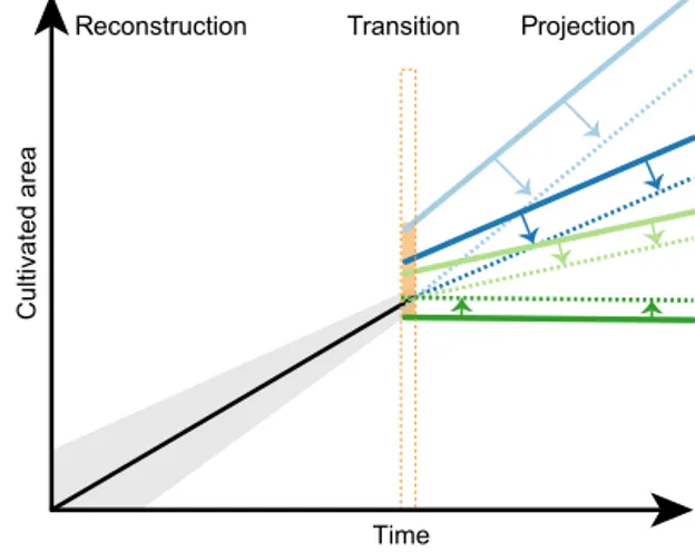
However, observational data on LULCC are not available on the global scale with the required temporal and spatial resolution, consistency, and historical coverage (Verburg et al., 2011). Instead, models are utilized to represent global land use and produce the required land-use change time se-ries. Land-use modeling is typically split up into histori-cal backcasting approaches and future scenario modeling. Both forward- and backward-looking models apply a range of different modeling approaches as well as different as-sumptions about drivers and the spatial allocation of land-use changes (National Research Council, 2014; Yang et al., 2014), and they are often initialized with different represen-tations of present-day land use (Prestele et al., 2016). Thus, even the models within one community (future or historical) do not provide consistent information on land use and land-use change over time, and a variety of independent datasets on a spatially explicit or world regional level are provided to the user community (e.g., climate modeling) (see Sup-plement Sect. S1 and Table S1 for examples of the histor-ical data). These historhistor-ical and future datasets are not con-nected and consistent in the transition period and entail a va-riety of uncertainties (Klein Goldewijk and Verburg, 2013) (Fig. 1). In consequence, these datasets disagree about the amount and the spatial pattern of land affected by human activity. Moreover, varying detail in classification systems, inconsistent definition of individual categories (e.g., forest or pasture), and individual model aggregation techniques, amplify the discrepancies among models (Alexander et al., 2017; Prestele et al., 2016).
2.2 Current approach to providing consistent data: the
Land-Use Harmonization (LUH) project
Large efforts have been undertaken to connect the differ-ent sources of land-use data and provide consistdiffer-ent time se-ries for climate modeling applications during the fifth phase of the Coupled Model Intercomparison Project (CMIP5; Taylor et al., 2012) by the LUH project (Hurtt et al., 2011). The resulting dataset (hereafter referred to as LUH data) is commonly used in modeling studies dealing with land use–climate interactions and feedbacks. It has recently been updated for the upcoming sixth phase of the Coupled Model Intercomparison Project (CMIP6; Eyring et al., 2016; Lawrence et al., 2016) and data for the historical period have been published (hereafter referred to as LUH2). Due to the
Figure 1.Simplified scheme of the harmonization process. Future projections from different models (solid colored lines) are smoothly connected (dashed colored lines) to the HYDE historical recon-struction (black line; grey shading represents the uncertainty range of LULCC history). Uncertainty about the extent and pattern of current land use and land cover (orange shading) is removed and the total area of cultivated land projected by the different models is changed.
lack of comprehensive documentation of the updated version at the time this paper was written and as, to our best knowl-edge, the points we demonstrate using LUH will still be valid with the new product, we primarily refer to the CMIP5 ver-sion in the remainder of this paper.
Hurtt et al. (2011) extended their Global Land-use Model (GLM; Hurtt et al., 2006) to produce a consistent time series of land-use states (fraction of each land-use category in a grid cell) and transitions (changes between land-use categories in a grid cell) for the time period 1500–2100. The cropland, pasture, and wood harvest projections of four IAMs were smoothly connected to the History Database of the Global Environment (HYDE) historical reconstruction of agricul-tural land use (Klein Goldewijk et al., 2011) and histori-cal wood harvest estimates by applying the decadal spatial patterns from the projections onto the HYDE map of 2005 (Fig. 1). This harmonization process tries to conserve the original patterns, rate, and location of change as much as possible and to reduce the differences between the models due to definition of cropland, pasture, and wood harvest. To achieve the final harmonized time series and explicit transi-tions, the preprocessed land-use time series are used as input into the GLM model and constrained by further data and as-sumptions about the occurrence of shifting cultivation, the spatial pattern of wood harvest, priority of the source of agri-cultural land, and biomass density (Hurtt et al., 2011). The harmonization ensured, for the first time, consistent land-use input for climate model intercomparisons and thus facilitated the implementation of anthropogenic impact on the land in climate models. Beyond this inarguable success, several un-certainties are to date not, or only partially, addressed in the
LUH data. In the following section we discuss the main un-certainties and how they may propagate into TBMs, impact-ing the amplitude and possibly even the sign of land-use in-teractions and feedbacks.
2.3 Open issues in the LUH data and their implications
for climate change assessments
The first major uncertainty of the LUH data evolves from the exclusive consideration of the HYDE baseline dataset for the historical period. The HYDE reconstruction is erroneously regarded as observational data rather than as model output accompanied by various sources of uncertainty (Klein Gold-ewijk and Verburg, 2013). Importantly, the LUH2 data will additionally include the HYDE low and high estimates of land use for the historical period (Lawrence et al., 2016). However, alternative spatially explicit reconstructions have been proposed (Kaplan et al., 2010; Pongratz et al., 2008; Ramankutty and Foley, 1999) (see Supplement Sect. S1 and Table S1 for additional information on these reconstruc-tions), and have been shown to differ substantially in terms of both the total cultivated area and spatial pattern over time (Meiyappan and Jain, 2012). These differences origi-nate in the scarcity of historical input data (i.e., mainly pop-ulation estimates) for historical times, the assumption about the functional relationship between population density and land use (e.g., linear or nonlinear), and the allocation scheme used to distribute regional or national estimates of agricul-tural land to specific grid cell locations (Klein Goldewijk and Verburg, 2013).
The uncertainty about land-use history has several im-plications for land use–climate interactions (Brovkin et al., 2004). For instance, Meiyappan et al. (2015) found the dif-ference in cumulative land-use emissions among three his-torical reconstructions for the 21st century modeled by one TBM to be about 18 PgC or ∼ 11 % of the mean land-use emission. Another study, using three commonly used net land-use datasets in one TBM, revealed differences of about 20 PgC or ∼ 9 % of the mean land-use emission since 1750 (Bayer et al., 2017). Jain et al. (2013) further found contrast-ing trends in land-use emissions on a regional scale durcontrast-ing the past 3 decades, which originate in different amounts and rates of land-use change in different realizations of histor-ical land use. Furthermore, as biophyshistor-ical climate impacts of land use are known to be substantial, especially on a re-gional scale (Alkama and Cescatti, 2016; Pielke et al., 2011; Pitman et al., 2009), an inappropriate representation of the uncertainty about land-use history is likely to affect model outcomes regarding changes in local to regional climate. Us-ing the HYDE reconstruction exclusively implies high confi-dence about land-use history in many large-scale assessments and comparison studies (Kumar et al., 2013; Le Quéré et al., 2015; Pitman et al., 2009); this confidence is in fact lack-ing. As a result, important uncertainties are excluded from
climate change mitigation and adaptation policies developed based on these studies (Mahmood et al., 2016).
Second, large inconsistencies exist between estimates of present-day land use. The LUH approach does not consider the differences between different data regarding the current state of land use as it connects the future projections exclu-sively to the HYDE end map (Fig. 1). The present-day start-ing maps of historical reconstructions and future projections are based on maps derived from the integration of remotely sensed land-cover maps and (sub-)national statistics of land use (e.g., Erb et al., 2007; Fritz et al., 2015; Klein Goldewijk et al., 2011; Ramankutty et al., 2008). The land-cover maps in turn disagree about extent and spatial pattern of agricul-tural land (Congalton et al., 2014; Fritz et al., 2011) due to both inconsistent definitions of individual use and land-cover categories (e.g., Sexton et al., 2015) and difficulties in identifying them from the spectral response (Friedl et al., 2010). These differences propagate into the starting maps of the various land-use change models, including the IAMs pro-viding data for the LUH (Prestele et al., 2016). Removing these differences can result in substantial deviations of the seasonal and spatial pattern of surface albedo, net radiation, and partitioning of latent and sensible heat flux (Feddema et al., 2005) and can affect carbon flux estimates proposed by TBMs across spatial scales (Quaife et al., 2008).
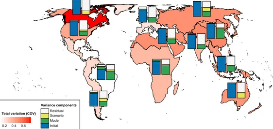
Finally, the future projections used in the LUH are pro-vided by different IAMs, whereby each of them represents an individual scenario of the four representative concentra-tion pathways (RCPs) in CMIP5 or the five shared socioe-conomic pathways (SSPs) in CMIP6 (O’Neill et al., 2017; van Vuuren et al., 2011). These are referred to as “marker scenarios” in the case of the SSPs. A marker scenario entails the implementation of a SSP by one IAM that was elected to represent the characteristics of the qualitative SSP storyline best, while additional implementations of the same SSP in other IAMs are “non-marker scenarios” (Popp et al., 2017; Riahi et al., 2017). Alternative RCP or SSP implementations were not considered in LUH. Land-use change model inter-comparisons and sensitivity studies, however, indicate that the uncertainty range emerging from different assumptions in the models, input data, and spatial configuration substantially impacts the model results (Alexander et al., 2017; Di Vitto-rio et al., 2016; Schmitz et al., 2014). Due to the large range across model outcomes per scenario, the problems of using marker scenarios from different models are evident. How-ever, no better alternative to this approach seems to be cur-rently available, and representing uncertainty across models is valuable (Popp et al., 2017). Model comparisons further revealed that while land-use change models represent the fu-ture development of cropland area more consistently, the rep-resentation of pastures and forests (if modeled) is poor. For example, the projections of 11 IAMs and LUCMs show large variations in pasture areas in 2030 for many world regions (Fig. 2, background map; Supplement Sect. S2.1). These pro-jections were based on a wide range of scenarios, and thus
Figure 2.Variation (expressed as coefficients of variation) in pasture projections for 12 world regions in 2030 (shading of the background map). The left bar plots show the relative contribution (as a percentage) of initial variation (pasture area in relation to values reported by FAO (2015) for the year 2010), model-related variation (model type and spatial configuration), and scenario-related variation to the total variation in a region. The right bar plots show the relative contribution (as a percentage) of variance components to the part of total variation that cannot be attributed to initial variation. The figure is based on 11 regional and spatially explicit land-use change models as described in Prestele et al. (2016). Methodological details can be found in Supplement Sect. S2.1 (Table S2) and in Alexander et al. (2017).
variation in outcomes was to be expected (Prestele et al., 2016). The variation attributed to the difference in model structure exceeds the variation due to different scenarios in most regions (Fig. 2, bar plots), while the main part of the variation relates to the different starting points of the mod-els, i.e., deviation from FAO pasture areas in the year 2010. This implies that in many cases the different land-use projec-tions actually do not represent different outcomes resulting from different scenario assumptions, but rather differences between land-use data input used to calibrate the models and the implementation of drivers and processes in the mod-els. Consequently, differences in future climate impacts of land use are likely also affected by the structural differences across land-use change models.
3 Challenge II: considering gross land-use changes
3.1 Background and emergence
Typically, net land-use changes are applied in TBMs. Net land-use changes refer to the summed grid cell difference in land-use categories between two subsequent time steps at a certain spatial and temporal resolution. Gross change rep-resentations provide additional information about land-use changes on a sub-grid scale. The total area in a grid cell that has been affected by change can be calculated by the sum of all individual changes (i.e., area gains and area losses). Gross changes have been shown to be substantially larger than net changes due to bidirectional change processes happening at the same time step (Fuchs et al., 2015a; Hurtt et al., 2011) that are obscured in net change representations. For example, 20 km2cropland at time t1and 40 km2at time t2within a grid
cell does not necessarily mean that this change resulted from clearing exactly 20 km2of forest. Equally plausible would be clearance of forest of larger spatial extent, while at the same time also abandoning a certain amount of cropland, resulting in the same net areal change.
Gross changes are not consistently defined across commu-nities. Commonly, shifting cultivation (mostly occurring to-day in parts of the tropics) and cropland–grassland dynam-ics (i.e., the bidirectional process of cropland expansion and abandonment) are referred to as gross changes (Fuchs et al., 2015a; Hurtt et al., 2011). Moreover, in the carbon cycle and climate modeling communities, wood harvest (in addi-tion to forest cleared for agricultural land) is sometimes in-cluded in gross changes (Hurtt et al., 2011; Stocker et al., 2014; Wilkenskjeld et al., 2014). A more general definition would include all area changes (i.e., gains and losses across all categories represented in a product) that are not depicted in land-use change products (Fuchs et al., 2015a). The larger the averaging unit (be it in terms of grid cell or time), the greater the discrepancy between gross and net changes be-comes. Re-gridding of high-resolution (e.g., 5 arcmin) land-use information to the TBM grid (∼ 0.5◦) thus entails addi-tional loss of information on land-use transitions unless gross changes are considered.
These sub-grid dynamics have been shown to be of impor-tance when modeling change of carbon and nutrient stocks in response to land-use change in recent TBM studies (Bayer et al., 2017; Fuchs et al., 2016; Stocker et al., 2014; Wilken-skjeld et al., 2014). For example, Bayer et al. (2017) found the global cumulative land-use carbon emission to be ∼ 33 % higher over the time period 1700–2014. Stocker et al. (2014)
likewise report increased carbon emissions in recent decades and for all RCPs when accounting for shifting cultivation and wood harvest. Similarly, Wilkenskjeld et al. (2014) found a 60 % increase in the annual land-use emission for the his-torical period (1850–2005) and a range of 16–34 % increase for future scenarios, when accounting for gross changes. Re-cently, Arneth et al. (2017) demonstrated uniformly larger historical land-use change carbon emissions across a range of TBMs when shifting cultivation and wood harvest were included, which has implications for understanding of the terrestrial carbon budget as well as for estimates of future carbon mitigation potential in regrowing forest.
Except for such sensitivity studies, gross changes have hardly been considered so far in land use–climate interac-tion studies (a notable excepinterac-tion being Shevliakova et al., 2013), mainly due to two reasons. First, gross change timates have not been available until recently. Deriving es-timates of historical and future gross change is a difficult task since gross changes vary with spatial and temporal scale (Fuchs et al., 2015a), i.e., they are dependent on the scale of the underlying net change product used for modeling and to what extent gross change processes are included in the indi-vidual land-use change models. Second, the implementation of bidirectional changes below the native model grid often entails substantial technical modification to TBM structure, meaning that many TBMs are currently not ready to include information on gross changes or only started recently to in-clude it.
3.2 Example: gross changes due to re-gridding in the
CLUMondo model
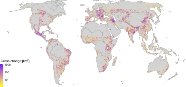
To illustrate the amount of land-use and land-cover change that might be missed in net representations, we conducted an analysis based on the output of a dedicated high-resolution LUCM (CLUMondo; 5 arcmin spatial resolution; Eitelberg et al., 2016; Van Asselen and Verburg, 2013). We tracked all changes between five land-use and land-cover categories (cropland, pasture, forest, urban, and bare) at the original res-olution over the time period from 2000 to 2040. Aggregat-ing to ca. 0.5◦ resolution allowed the differentiation of the gross area from the net area affected by change (see Sup-plement Sect. S2.2 for methodological details). The results, shown in Fig. 3, indicate that gross changes are substantially higher than net changes all over the globe, including the tem-perate zone and high latitudes. It has to be noted that Fig. 3 is only based on one realization of a single LUCM, i.e., not necessarily representing the full extent and spatial pattern of global-scale gross changes. The analysis only depicts the loss of information while re-gridding from 5 arcmin to 0.5◦ reso-lution. Thus, bidirectional changes below the spatial resolu-tion of the original data are still not captured.
3.3 Current approaches to providing gross change
information: LUH and analysis of empirical data
To provide estimates of gross change, the land-use change modeling community currently follows two different ap-proaches. First, Hurtt et al. (2011), within the framework of LUH, propose a matrix that provides explicit transitions be-tween cropland, pasture, urban, and natural vegetation. Sub-grid-scale information is added to net transitions (that are de-rived from historical or projected land-use data and referred to as “minimum transitions”) through assumptions about the extent of shifting cultivation practices and the spatial pattern of wood harvest. In each grid cell, where shifting cultiva-tion appears according to a map of Butler (1980), an average land-abandonment rate is added to each transition from and to agricultural land. In LUH2 an updated shifting-cultivation estimate based on the analysis of Landsat imagery will be included and replace the aforementioned simple assumption (Lawrence et al., 2016). Wood harvest is regarded as gross change, if the wood harvest demand from statistics (histori-cal) or IAMs (future) is not met by deforestation for agricul-tural land in the net transitions or the GLM model is run in a configuration where deforestation for agricultural land is not counted towards wood harvest demand.
The second approach derives gross / net ratios and a tran-sition matrix directly from empirical data such as histori-cal maps or high-resolution remote sensing products. These ratios can subsequently be applied to existing historical or future net representations to provide estimates of additional area affected by change (Fuchs et al., 2015a).
3.4 Open issues in the current approaches
The LUH gross transitions account for some aspects of gross changes. However, the values are dependent on what one in-cludes in the definition of gross changes and are based on overly simplistic assumptions. Most of the gross transitions appear in parts of the tropics, where shifting cultivation is as-sumed to be an important agricultural practice (Bayer et al., 2017; their Fig. S1). Gross changes outside of these areas are mainly related to wood harvest, i.e., the (additional) area de-forested to meet external wood harvest demands. Although these are regarded as gross changes in some literature (e.g., Hurtt et al., 2011; Stocker et al., 2014), we argue that wood harvest not leading to an actual areal change of land cover (e.g., forest to cropland) should be referred to as land man-agement rather than gross change. Excluding wood harvest from the LUH data restricts the occurrence of gross changes to the areas of shifting cultivation. However, our analysis of CLUMondo output (Fig. 3), along with the European analy-sis of Fuchs et al. (2015a), suggests substantial amounts of gross change (below the 0.5◦LUH grid) also in the temper-ate zone and the high latitudes. Consequently, the LUH ap-proach heavily depends on the resolution of the original land-use data (provided by IAMs or historical reconstructions) and
Figure 3. Difference between gross versus net area affected by change at grid cell level (ca. 0.5◦×0.5◦) as shown by one realization of a single LUCM (CLUMondo; FAO 3 demand scenario). Areas affected by net or gross change have been accumulated over a 40-year simulation period (2000–2040). Net changes are calculated at ca. 0.5◦×0.5◦resolution, while gross changes also account for bidirectional changes at the 5 arcmin native CLUMondo resolution (Supplement Sect. S2.2; Fig. S1). Darker colors indicate a larger difference between the area changed under net and gross change views at ca. 0.5◦×0.5◦grid level. Note the logarithmic scale.
their ability to represent land-use change dynamics on a sub-grid scale.
The data-based approach avoids the process uncertainty that hinders high-resolution model projections of land use, but is limited to the time period where empirical data through remote sensing is available. Additional sources such as his-torical land-use and land-cover maps and statistics (Fuchs et al., 2015b) may contribute to covering longer time pe-riods, although with limited spatiotemporal resolution and spatial coverage, and an associated increase in uncertainty. It is thus difficult to develop multi-century reconstructions or future scenarios including gross changes using data-based approaches since the derived gross / net ratios are only valid for periods of data coverage and are expected to change over time (Fuchs et al., 2015a).
4 Challenge III: allocation of managed land in TBMs
4.1 Background and emergence
The LSMs in most Earth system models (ESMs) in CMIP5 treated the land surface as a static representation of current land-use and land-cover distribution typically derived from remote sensing products (Brovkin et al., 2013; de Noblet-Ducoudré et al., 2012). DGVMs, some of which are incor-porated in the land surface component of ESMs, were orig-inally designed to model potential natural vegetation as a dynamic function of monthly climatology, bioclimatic lim-its, soil type, and the competitiveness of different wood- or grass-shaped plant functional types (PFTs) (Prentice et al., 2007). Thus, the early TBMs were not able to sufficiently account for anthropogenic activity on the land surface and
consequently the impact of land use on climate and bio-geochemical cycles (Flato et al., 2013). However, over the last decade, representation of human land-cover change and also some land-management aspects have increasingly been added to these models, albeit with levels of complexity that vary from crops as grassland to more detailed agricultural representations (Bondeau et al., 2007; Le Quéré et al., 2015; Lindeskog et al., 2013). Crop functional types (CFTs) and management options have been introduced in some mod-els, explicitly parameterizing the phenology and biophysical and biogeochemical characteristics of major crop types and distinguishing important management options such as irriga-tion, fertilizer applicairriga-tion, occurrence of multiple cropping, or processing of crop residues (Bondeau et al., 2007; Lin-deskog et al., 2013). However, since TBMs do not include representations of human activity as a driver of changes in the land surface, information about the extent and exact loca-tion of managed land is required from external data sources such as IAMs or LUCMs.
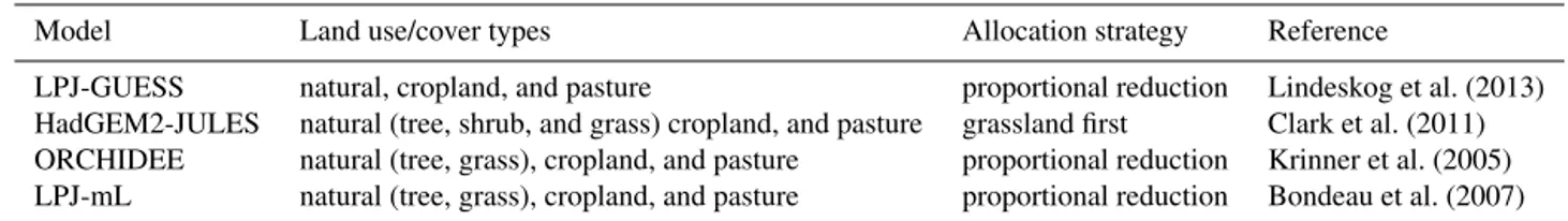
IAMs and LUCMs usually provide land-cover information (e.g., forest, grassland, and shrubland) along with land-use information (e.g., cropland and pasture). However, as mod-eling changes in natural vegetation type is one of the pri-mary functions of many TBMs, only land-use information has been used in the LUH (Hurtt et al., 2011). Hence, TBM modelers have to decide in which way the natural vegeta-tion in a grid cell has to be reduced (in case of expansion of managed land) or increased (in case of abandonment of man-aged land). This has resulted in a range of different strate-gies, which we show as an illustration in Table 1 for a non-exhaustive list of models. The decision is important as it
im-Table 1.Examples of allocation rules at grid cell level to implement agricultural land in different TBMs.
Model Land use/cover types Allocation strategy Reference
LPJ-GUESS natural, cropland, and pasture proportional reduction Lindeskog et al. (2013) HadGEM2-JULES natural (tree, shrub, and grass) cropland, and pasture grassland first Clark et al. (2011) ORCHIDEE natural (tree, grass), cropland, and pasture proportional reduction Krinner et al. (2005) LPJ-mL natural (tree, grass), cropland, and pasture proportional reduction Bondeau et al. (2007)
pacts the distribution of the natural vegetation in a grid cell, as well as the mean length of time that land has been un-der a particular use, with consequences for both the biogeo-chemical and biophysical properties (Reick et al., 2013). For example, new cropland expanding into forest would lead to a large and relatively rapid loss of ecosystem carbon due to de-forestation, while cropland expanding into former grassland would have a less immediate impact on ecosystem carbon stocks due to the long time lag (years to centuries) for the resulting changes in soil carbon to be realized (Pugh et al., 2015). Likewise, the albedo and partitioning of energy differs strongly between forest and grassland land covers (Mahmood et al., 2014; Pielke et al., 2011). In the following sections we illustrate, based on literature review and analysis of empir-ical and modeled data, that the previously described simple allocation algorithms, applied globally within TBMs, do not account well for the spatiotemporal variation in land-use and land-cover change.
4.2 Spatial heterogeneity of cropland transitions –
empirical evidence
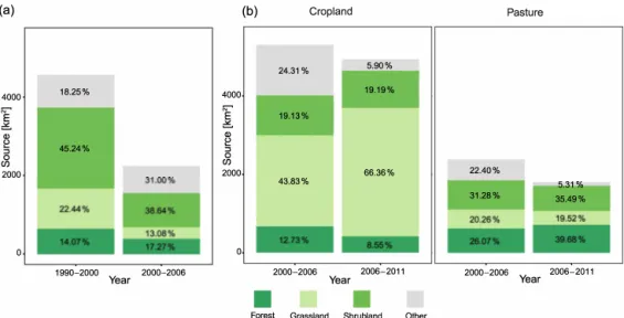
Table 2 summarizes dominant sources of cropland expansion for several world regions and demonstrates the heterogeneity in the spatial pattern of expanding agriculture. For Europe, the CORINE land-cover product (Bossard et al., 2000) indi-cates over two consecutive time periods (1990–2000, 2000– 2006) shrubland systems to be the main source of expand-ing agricultural land, followed by low-productivity grass-lands and forests (Fig. 4a). In contrast, over a similar time period, the NLCD (Homer et al., 2015) for the USA shows low-productivity grasslands as the dominant source of new croplands, while pastures are predominantly converted from forest or shrubland systems and grasslands only account for around 20 % of new pastures (Fig. 4b). A large-scale study by Graesser et al. (2015) covering Latin America and based on the interpretation of MODIS images for the time period 2001–2013 identified the dominant trajectory of forests be-ing first converted to pastures and subsequently to cropland. They show, however, varying patterns on national and ecore-gional scales. This reecore-gional variation is also emphasized by Ferreira et al. (2015), who describe a satellite-based transi-tion matrix as input for a modeling study for different states in Brazil. They do not distinguish non-forest natural vegeta-tion such as the Cerrado systems, which might be another
im-portant source for agricultural land (Grecchi et al., 2014). A study conducted by Gibbs et al. (2010) investigating agricul-tural expansion in the tropics in the 1980s and 1990s based on data from the Food and Agriculture Organization of the United Nations (2000) (i.e., areas with less than 10 % for-est cover are not considered) concludes that more than 80 % of new agricultural land originates from intact or degraded forests. Gibbs et al. (2010) further found large variability in agricultural sources across seven major tropical regions, e.g., substantially higher conversions from shrublands and woodlands to agricultural land in South America and eastern Africa. Grasslands have been detected as the main source of agricultural land in northern China, e.g., by Li (2008), Liu et al. (2009), and Zuo et al. (2014), while in the Yangtze River basin woodlands contribute most (Wu et al., 2008) (Table 2). All the studies mentioned indeed combine differ-ent approaches to derive changes, cover differdiffer-ent time peri-ods, and are not representative of current agricultural change hotspots (Lepers et al., 2005). However, this kind of aggre-gated analysis already indicates that the spatial pattern of agricultural change dynamics varies across world regions and a single global algorithm to replace natural vegetation by managed land in TBMs is likely to be overly simplistic.
4.3 Example: spatial heterogeneity of cropland
transitions in the CLUMondo model
As it is not possible to compare the land-use allocation strategies of TBMs with historical change data on a global scale due to the lack of accurate global use and land-cover products (though products with higher resolution (up to ∼ 30 m), more frequent temporal coverage, and increas-ing thematic detail are just emergincreas-ing; Ban et al., 2015), we additionally tested to what extent cropland expansion simu-lated by the land-use change model CLUMondo (Eitelberg et al., 2016; Van Asselen and Verburg, 2013) represents one or more of the simplified algorithms currently considered in TBMs (Table 1).
CLUMondo models the spatial distribution of land sys-tems over time, instead of land use and land cover directly. Land systems are characterized by, in addition to other fac-tors, a mosaic of land use and land cover within each grid cell. The land systems are allocated to the grid in each time step “based on local suitability, spatial restrictions, and the competition between land systems driven by demands for
(a) 4000 � E � Q) (.) ::J 0 (/) 2000 0 18.25% 45.24% 1990-2000 2000-2006 Year 4000 � E � Q) (.) L. ::J 0 (/) 2000 0 (b)
II
Cropland 24.31 % 5.90% 19.19% 19.13% 66.36% 43.83% 2000-2006 2006-2011 YearII
Forest Grassland Shrubland Other
Pasture 22.40% 5.31 % 31.28% 35.49% 2000-2006 2006-2011 Year
Figure 4.Sources of agricultural land (cropland and pasture combined) for two time periods in Europe based on the CORINE land-cover data (a) and sources of cropland and pasture for two time periods in the USA based on the NLCD land-cover data (b) (Supplement Sect. S2.3, Table S3). Changes between different agricultural classes are not considered as expansion of agricultural land. Aggregation of CORINE and NLCD legends to forest, grassland, and shrubland is according to Tables S4–5. The category “other” includes urban land, wetlands, water, and bare land.
Table 2.Case studies and continental-scale remote sensing studies that report main sources of agricultural expansion or allow for land-cover change detection.
Region Temporal coverage Main source of new cropland
Main source of new pasture
Reference
Europe 1990–2000/ Shrubland/ Shrubland/ Bossard et al. (2000) 2000–2006 Shrubland∗ Shrubland∗ USA 2001–2006/ 2006–2011 Grassland/ Grassland Shrubland/ Forest Homer et al. (2015) Latin America 2001–2013 Pasture Forest Graesser et al. (2015) Northern China 1989–1999/ Grassland/ – Li (2008)
1999–2003 Grassland
1986–2000 Grassland – Liu et al. (2009) 1995–2010 Grassland – Zuo et al. (2014) Yangtze River basin 1980–2000 Woodland – Wu et al. (2008) Brazil 1994–2002 Forest Forest Ferreira et al. (2015) Tropics 1980–2000 Forest∗ Forest∗ Gibbs et al. (2010)
∗Source refers to all new agricultural land, i.e., cropland and pasture combined.
different goods and services” (Eitelberg et al., 2016; Van Asselen and Verburg, 2013). Thus, the determination of the source land use or land cover upon cropland expansion can be interpreted as a complex algorithm taking into account external demands, the land-use distribution of the previous time step, local suitability in a grid cell, and neighborhood effects (i.e., cropland expansion in a grid cell also depends on the availability of suitable land in the surrounding grid cells). This strategy differs from the one in TBMs in a way that not one simple rule is applied to each grid cell equally, but accounts for the spatial heterogeneity of drivers of land-use change.
In order to compare the sources of cropland expansion in CLUMondo to the globally applied rules in TBMs, we re-classified the outputs of the same CLUMondo simulation uti-lized in Sect. 3.2 (FAO3D; Eitelberg et al.; 2016) according to their dominant land-use or land-cover type to derive tran-sitions (Table S6) and classified the changes within each ca. 0.5◦×0.5◦grid cell as either grassland first, forest first, pro-portional, or a complex reduction pattern (Table 3; Fig. S2–3 and additional explanation in Supplement Sect. S2.4). Ad-ditionally, a grid cell was labeled undefined if grassland or forest was not available in the source map.
Figure 5 shows the results of this analysis for decadal time steps between 2000 and 2040. Based on the CLUMondo
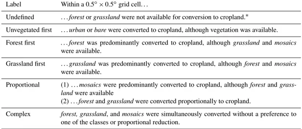
Table 3.Definition of classified algorithms in the CLUMondo exercise (Sect. 4.3). CLUMondo data were preprocessed as described in the text and Supplement Sect. S2.4. Each ca. 0.5◦×0.5◦grid cell was assigned a label according to the distribution of changes seen in the higher resolution (5 arcmin) CLUMondo data. Land types according to the reclassification of CLUMondo land systems are shown in Table S6; mosaics refer to a mixture of vegetation within a grid cell (e.g., forest and grassland).
Label Within a 0.5◦×0.5◦grid cell. . .
Undefined . . . forest or grassland were not available for conversion to cropland.∗
Unvegetated first . . . urban or bare were converted to cropland, although vegetation was available. Forest first . . . forestwas predominantly converted to cropland, although grassland and mosaics
were available.
Grassland first . . . grassland was predominantly converted to cropland, although forest and mosaics were available.
Proportional (1) . . . mosaics were predominantly converted to cropland, although forest and grass-landwere available
(2) . . . forest and grassland were converted proportionally to cropland.
Complex forest, grassland, and mosaics were simultaneously converted without a preference to one of the classes or proportional reduction.
∗If one of the two classes is not available for conversion, either of the preferential algorithms (unvegetated, forest, or grassland first) could be
correct, but not executed because of the lack of the source that should be converted first.
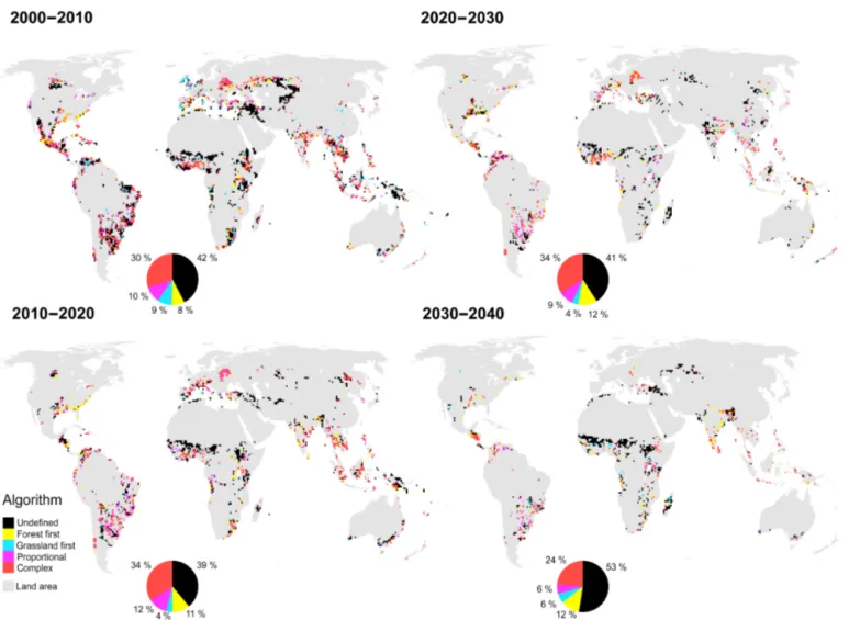
data, it is clear that a single simple algorithm does not ac-count for the temporal and spatial heterogeneity of cropland expansion in a detailed land-use change model. The major-ity of grid cells with substantial cropland expansion (> 10 % of grid cell area) where we could detect an algorithm (i.e., the grid cell was not classified undefined) show a complex reduction pattern of the remaining land-use and land-cover categories, i.e., any algorithm applied to these grid cells in a TBM could be seen as equally good or bad. The remain-ing grid cells account for only 24–27 % globally. Moreover, the spatial distribution of grid cells that are classified to the same algorithm is very heterogeneous and changes over time. It has to be noted that this analysis builds on only one real-ization of one LUCM and results may differ if using another data source in terms of overall cropland expansion and the exact grid cell location of changes. However, the analysis does not aim at identifying the exact location of a partic-ular algorithm but rather at emphasizing the heterogeneous pattern of cropland expansion.
4.4 Current approach to providing allocation
information: the transition matrix
In CMIP5, most ESMs implemented a proportional reduc-tion of natural vegetareduc-tion rather arbitrarily due to reasons of simplicity or internal model constraints; others converted grassland preferentially and/or treated croplands differently from pastures upon transformation (de Noblet-Ducoudré et al., 2012). However, none of them depict the complex inter-play of biophysical and socioeconomic parameters leading to a heterogeneous spatial pattern of land-use change within the coarse grid resolution used in ESMs. As we have shown
in the previous sections, empirical evidence and land-use change models suggest that this complexity is poorly repre-sented by simplistic, globally applied algorithms. The efforts of LUH thus included the provision of a transition matrix, i.e., the explicit identification of source and target categories between agricultural land and natural vegetation at the grid cell level. For each annual time step, the exact fraction of a grid cell that has changed from one land-use category to another is determined, thus providing the option to replace the simple allocation options with detailed information about land-use transitions within each grid cell (Hurtt et al., 2011).
4.5 Open issues of transition matrices
The provision of transition matrices, however, generally brings up a sequence of additional challenges, which we il-lustrate using the example of LUH in the following. First, the decision of which land-cover type should be replaced upon cropland or pasture expansion (or introduced in case of abandonment) is in fact only shifted from the TBM commu-nity to the IAM/LUCM commucommu-nity and the accuracy of the transitions are heavily dependent on the sophistication (i.e., knowledge about and depiction of land-use change drivers and processes on the grid scale) of the land-use allocation algorithm in the original model providing the land-use data. Many current models simulate land-use changes on a world regional level and downscale these aggregated results to the required grid cell level (Hasegawa et al., 2016; Schmitz et al., 2014). In the LUH approach these downscaled data are used to derive the minimum transitions between agricultural land use and natural vegetation. Additional assumptions are made to allocate changes in land-use states to explicit
tran-Figure 5.Transitions from natural vegetation to cropland as shown by the CLUMondo model (FAO 3 demand scenario) from 2000 to 2040 in decadal time steps. Colored grid cells represent areas with at least 10 % of cropland expansion within a ca. 0.5◦×0.5◦grid cell. Grid cells are classified according to forest-first (yellow), grassland-first (cyan), proportional (magenta), and complex (red) reduction algorithms as described in the text (for details see Supplement Sect. S2.4). Black grid cells denote areas where the validity of no algorithms could be detected. Grid cells classified as unvegetated first (Table 3) are not shown due to a very small contribution (< 0.1 %). Grid cells in this figure have been aggregated to ca. 1.0◦×1.0◦following a majority resampling for reasons of readability. A high-resolution version of the maps, including the full detail of the classification results, can be found in the Supplement (Fig. S4).
sitions, not accounting for the spatial and temporal hetero-geneity of the multiple drivers of land-use change. For exam-ple, urban expansion is applied proportionally to cropland, pasture, and (secondary) natural vegetation. Upon transitions between natural vegetation and agricultural land, choices in the model configuration have to be made, whether primary or secondary land is converted preferentially. These choices are similar to the grassland- or forest-first reduction algorithms applied in TBMs.
Moreover, due to the lack of empirical long-term, highly accurate land-use and land-cover change information and the inconsistencies between agricultural use data and land-cover information from satellites, global IAMs and LUCMs are rarely evaluated against independent data (Verburg et al., 2015). It is thus not clear yet to what extent the spatial
land-use patterns simulated by these models and provided to LUH represent a good estimate of real past and future land-use changes. In consequence, transitions derived from these modeled time series are uncertain.
Hence, it is evident that more and improved empirical information on land-use transitions is required to improve land-use change modeling and to estimate the natural sys-tems at risk under agricultural expansion. However, the spe-cific problem of allocating new agricultural land in DGVMs and LSMs also has strong model and data-structure compo-nents. In many DGVMs, the grass and forest PFTs on non-agricultural land in a grid cell are mostly not considered dif-ferent systems, but are part of one complex vegetation struc-ture thus not representing spatially horizontal heterogeneity. Therefore, when agriculture expands into such natural
sys-tems, all natural PFTs need to be reduced proportionally. If handled otherwise (i.e., when removing a specific PFT pref-erentially), the vegetation dynamics would slowly converge again towards the initial PFT mix (if all boundary conditions like climate and soil properties remain unchanged).
For LSMs coupled to ESMs, the situation is slightly more complex. Most ESMs (if not incorporating dynamic vegeta-tion through a DGVM) use a remote sensing product such as the ESA CCI-LC (ESA, 2014) and a translation to PFTs, e.g., Poulter et al. (2011), as a background vegetation map on which agricultural land is imposed. Due to inaccuracies in global remote sensing land-cover products and differences in historical reconstructions (as discussed in Sect. 2), frac-tions of agricultural land on a grid scale are subject to differ-ences between the background map and the external land-use dataset. Consequently, the PFT composition outside the pre-scribed agricultural land can represent either the real hetero-geneity in natural vegetation or represent a mix of natural and anthropogenic land cover due to differences in the datasets. However, these cases are difficult to distinguish and empir-ically justified transition matrices, together with more accu-rate present-day land-cover products, would provide a useful tool for reducing uncertainties due to allocation decisions in ESMs.
5 Recommendations for improving the current LULCC representation across models
5.1 Tackling uncertainties in the harmonization
The LUH (Hurtt et al., 2011) has allowed the inclusion of an-thropogenic impacts on the land surface for the first time in the CMIP5 climate change assessments. As we have shown in Sect. 2, three major sources of uncertainty, which in-clude the uncertainty about land-use history, inconsistencies in present-day land-use estimates, and structural differences across IAMs and LUCMs, are poorly addressed through the almost exclusive implementation of the LUH dataset within the climate modeling community. A wider range of harmo-nized time series is therefore likely to substantially influence the outcomes of studies on land use–climate interactions. The actual impact of alternative harmonized time series on car-bon cycle (and other ecosystem processes) and climate has never been tested, mainly due to the lack of alternative pro-vision of such products. One would need a multi-model en-semble design to properly account for and disentangle the in-dividual contributions of different historical reconstructions, the multitude of present-day land-use products, and varying future land-use change modeling approaches. Different fu-ture scenario models would need to be connected to differ-ent instances of historical reconstructions, both constrained by different plausible realizations (i.e., based on previously published, peer-reviewed approaches) of current land use and land cover. Such an approach would ensure a comprehensive coverage of the uncertainties accumulating across temporal
and spatial scales prior to feeding land-use data into climate models and allow for testing of climate model sensitivity to different realizations of land-cover and land-use information. The high computational demands of complex ESMs prob-ably do not allow for multiple runs including all the uncer-tainties in land-use forcing. However, to derive robust results from climate model intercomparisons, a sufficient quantifi-cation of uncertainty in the land-use forcing dataset is ur-gently required. If this proves impractical through ESM sim-ulations, we recommend utilizing less computationally ex-pensive models such as DGVMs and offline LSMs to assess the full range of uncertainty and to determine a limited set of simulations, which appears to significantly affect biogeo-chemical cycles and climate. These can be subsequently used to test the uncertainty range in ESMs.
Simultaneously, we suggest that the land-use and remote-sensing communities should engage to reduce uncertainties in land-use and land-cover products by
1. developing diagnostics for the evaluation of land-use reconstructions based on satellite data and additional proxy data such as pollen reconstructions (Gaillard et al., 2010) or archeological evidence of early land use (Kaplan et al., 2016);
2. developing systematic approaches to evaluating results of land-use change models against independent data sources, utilizing the full range of high-resolution satel-lite data (e.g., the Landsat archive and the European Sentinel satellites), reference data obtained from (sub-)national reporting schemes under international policy frameworks (e.g., Kohl et al., 2015), and innovative methods such as volunteered geographic information and crowdsourcing (Fritz et al., 2012). Although satel-lite data are also not directly measured empirical data, but go through a mathematical conversion process prior to a final land-cover product, they can improve repre-sentations of present-day land cover. If not yet possible on the global scale due to the limitations discussed in Sect. 2, we recommend the implementation of regional-scale evaluation schemes using smaller-regional-scale, highly ac-curate remote sensing products as a starting point for later integration into global applications.
5.2 Gross change representations
The full extent of gross changes is still not well understood (see Sect. 3). Thus, the land-use community should explore high-resolution remote-sensing imagery regarding their abil-ity to derive gross change estimates and improve understand-ing of sub-grid dynamics, which are not yet captured by their models. Regions where driving factors of small-scale land-use change processes are more complex and not easy to de-termine due to frequent land-use changes should receive spe-cial attention. Based on such analyses, multi-century recon-structions and projections for climate and ecosystem
assess-ments could be enhanced for at least the satellite era. As mod-els extend further into the past, the detailed information could be gradually replaced by model assumptions, supported by additional reference data such as historical maps and statis-tics.
5.3 Transition matrix from empirical data
Explicit information of land-use transitions instead of annual land-use states is essential for questions regarding carbon and nutrient cycling. We argue that simple, globally applied as-sumptions about these transitions or the shift of the respon-sibility from TBMs to land-use models may not solve the problem (Sect. 4). Thus, the development of dedicated tran-sition matrices increasingly based on empirical data (as soon as new products emerge) and sophisticated land-use change allocation models, which account for the spatiotemporal het-erogeneity of land-use change drivers, is essential.
Simultaneously, TBMs must ensure the use of the full de-tail of information provided by the implementation of ex-plicit transition information in their land modules. Due to in-ternal model structure, proportional reduction of PFTs needs to be applied in models with internally simulated dynamic vegetation. However, we recommend the utilization of ex-plicit transition information to further evaluate discrepancies between the potential natural vegetation scheme and LULCC data provided by LUCMs and IAMs.
6 Outlook: towards model integration across disciplines
The ways forward listed in the previous section will only be the first stage of a process towards improved LULCC representation in climate change assessments. Rather than improving de-coupled data products and models on an in-dividual basis and connecting them offline through the ex-change of files, we argue that land use, land cover, and the climate system need to be studied in an integrated model-ing framework. As we have shown in this paper, most of the challenges and related uncertainties originate in the dis-parate disciplinary treatment of the individual aspects. Al-though sophisticated models have been developed during the past decades within each community, the current offline cou-pling seems overly limited, accumulating an increasing level of uncertainty along the modeling chain. Integration of these different types of models, where anthropogenic activity on the land system is considered as an integral part of ESMs, instead of an external boundary condition, might help to re-duce these uncertainties, although it will certainly further complicate the interpretation of model responses. For ex-ample, Di Vittorio et al. (2014) report preliminary results of the iESM (Collins et al., 2015), an advanced coupling of an IAM and an ESM implementing two-way feedbacks be-tween the human and environmental systems, and show how this improved coupling can increase the accuracy of
infor-mation exchange between the individual model components. In the long term, additionally including behavioral land sys-tem models (e.g., agent-based approaches) in the coupling may provide further understanding of possible land–climate– society feedbacks (Arneth et al., 2014; Verburg et al., 2015) since the current modeling chain rarely accounts for the com-plexity of human–environmental relationships and feedbacks (Rounsevell et al., 2014).
Data availability. The illustrative analysis in Sects. 3 and 4 is based on CLUMondo simulations (Eitelberg et al., 2016). CLU-Mondo source code and simulation results are available from http: //www.environmentalgeography.nl/site/data-models/.
The Supplement related to this article is available online at doi:10.5194/esd-8-369-2017-supplement.
Competing interests. The authors declare that they have no con-flict of interest.
Acknowledgements. The research in this paper has been supported by the European Research Council under the Euro-pean Union’s Seventh Framework Programme project LUC4C (grant no. 603542), ERC grant GLOLAND (no. 311819), and BiodivERsA project TALE (no. 832.14.006) funded by the Dutch National Science Foundation (NWO). This research contributes to the Global Land Programme (www.glp.earth). This is paper number 26 of the Birmingham Institute of Forest Research. Edited by: R. A. P. Perdigão
Reviewed by: J. Hall and two anonymous referees
References
Alexander, P., Prestele, R., Verburg, P. H., Arneth, A., Baranzelli, C., Batista e Silva, F., Brown, C., Butler, A., Calvin, K., Den-doncker, N., Doelman, J. C., Dunford, R., Engström, K., Eitel-berg, D., Fujimori, S., Harrison, P. A., Hasegawa, T., Havlik, P., Holzhauer, S., Humpenöder, F., Jacobs-Crisioni, C., Jain, A. K., Krisztin, T., Kyle, P., Lavalle, C., Lenton, T., Liu, J., Meiyappan, P., Popp, A., Powell, T., Sands, R. D., Schaldach, R., Stehfest, E., Steinbuks, J., Tabeau, A., van Meijl, H., Wise, M. A., and Roun-sevell, M. D. A.: Assessing uncertainties in land cover projec-tions, Glob. Chang. Biol., 23, 767–781, doi:10.1111/gcb.13447, 2017.
Alkama, R. and Cescatti, A.: Biophysical climate impacts of recent changes in global forest cover, Science, 351, 600–604, 2016. Arneth, A., Harrison, S. P., Zaehle, S., Tsigaridis, K., Menon, S.,
Bartlein, P. J., Feichter, J., Korhola, A., Kulmala, M., O’Donnell, D., Schurgers, G., Sorvari, S., and Vesala, T.: Terrestrial biogeo-chemical feedbacks in the climate system, Nat. Geosci., 3, 525– 532, 2010.
Arneth, A., Brown, C., and Rounsevell, M. D. A.: Global models of human decision-making for land-based mitigation and adaptation assessment, Nature Climate Change, 4, 550–557, 2014. Arneth, A., Sitch, S., Pongratz, J., Stocker, B. D., Ciais, P., Poulter,
B., Bayer, A. D., Bondeau, A., Calle, L., Chini, L. P., Gasser, T., Fader, M., Friedlingstein, P., Kato, E., Li, W., Lindeskog, M., Nabel, J. E. M. S., Pugh, T. A. M., Robertson, E., Viovy, N., Yue, C., and Zaehle, S.: Historical carbon dioxide emissions caused by land-use changes are possibly larger than assumed, Nat. Geosci., 10, 79–84, 2017.
Ballantyne, A. P., Andres, R., Houghton, R., Stocker, B. D., Wan-ninkhof, R., Anderegg, W., Cooper, L. A., DeGrandpre, M., Tans, P. P., Miller, J. B., Alden, C., and White, J. W. C.: Audit of the global carbon budget: estimate errors and their impact on uptake uncertainty, Biogeosciences, 12, 2565–2584, doi:10.5194/bg-12-2565-2015, 2015.
Ban, Y. F., Gong, P., and Gini, C.: Global land cover mapping us-ing Earth observation satellite data: Recent progresses and chal-lenges, Isprs J. Photogramm., 103, 1–6, 2015.
Bayer, A. D., Lindeskog, M., Pugh, T. A. M., Anthoni, P. M., Fuchs, R., and Arneth, A.: Uncertainties in the land-use flux result-ing from land-use change reconstructions and gross land tran-sitions, Earth Syst. Dynam., 8, 91–111, doi:10.5194/esd-8-91-2017, 2017.
Bondeau, A., Smith, P. C., Zaehle, S., Schaphoff, S., Lucht, W., Cramer, W., Gerten, D., Lotze-Campen, H., Muller, C., Reich-stein, M., and Smith, B.: Modelling the role of agriculture for the 20th century global terrestrial carbon balance, Glob. Change Biol., 13, 679–706, 2007.
Bossard, M., Feranec, J., and Otahel, J.: CORINE land cover tech-nical guide – Addendum 2000, Techtech-nical Report, 40, 2000. Brovkin, V., Sitch, S., von Bloh, W., Claussen, M., Bauer, E., and
Cramer, W.: Role of land cover changes for atmospheric CO2 increase and climate change during the last 150 years, Glob. Change Biol., 10, 1253–1266, 2004.
Brovkin, V., Boysen, L., Arora, V. K., Boisier, J. P., Cadule, P., Chini, L., Claussen, M., Friedlingstein, P., Gayler, V., van den Hurk, B. J. J. M., Hurtt, G. C., Jones, C. D., Kato, E., de Noblet-Ducoudre, N., Pacifico, F., Pongratz, J., and Weiss, M.: Effect of Anthropogenic Land-Use and Land-Cover Changes on Climate and Land Carbon Storage in CMIP5 Projections for the Twenty-First Century, J. Climate, 26, 6859–6881, 2013.
Butler, J. H.: Economic Geography: Spatial and Environmental As-pects of Economic Activity, John Wiley, New York, 1980. Canadell, J. G., Le Quéré, C., Raupach, M. R., Field, C. B.,
Buiten-huis, E. T., Ciais, P., Conway, T. J., Gillett, N. P., Houghton, R. A., and Marland, G.: Contributions to accelerating atmospheric CO2growth from economic activity, carbon intensity, and effi-ciency of natural sinks, P. Natl. Acad. Sci. USA, 104, 18866– 18870, doi:10.1073/pnas.0702737104, 2007.
Clark, D. B., Mercado, L. M., Sitch, S., Jones, C. D., Gedney, N., Best, M. J., Pryor, M., Rooney, G. G., Essery, R. L. H., Blyth, E., Boucher, O., Harding, R. J., Huntingford, C., and Cox, P. M.: The Joint UK Land Environment Simulator (JULES), model descrip-tion – Part 2: Carbon fluxes and vegetadescrip-tion dynamics, Geosci. Model Dev., 4, 701–722, doi:10.5194/gmd-4-701-2011, 2011. Collins, W. D., Craig, A. P., Truesdale, J. E., Di Vittorio, A. V.,
Jones, A. D., Bond-Lamberty, B., Calvin, K. V., Edmonds, J. A., Kim, S. H., Thomson, A. M., Patel, P., Zhou, Y., Mao, J.,
Shi, X., Thornton, P. E., Chini, L. P., and Hurtt, G. C.: The in-tegrated Earth system model version 1: formulation and func-tionality, Geosci. Model Dev., 8, 2203–2219, doi:10.5194/gmd-8-2203-2015, 2015.
Congalton, R. G., Gu, J. Y., Yadav, K., Thenkabail, P., and Ozdo-gan, M.: Global Land Cover Mapping: A Review and Uncer-tainty Analysis, Remote Sensing, 6, 12070–12093, 2014. Davidson, E. A.: The contribution of manure and fertilizer nitrogen
to atmospheric nitrous oxide since 1860, Nat. Geosci., 2, 659– 662, 2009.
de Noblet-Ducoudré, N., Boisier, J. P., Pitman, A., Bonan, G. B., Brovkin, V., Cruz, F., Delire, C., Gayler, V., van den Hurk, B. J. J. M., Lawrence, P. J., van der Molen, M. K., Muller, C., Reick, C. H., Strengers, B. J., and Voldoire, A.: Determining Robust Impacts of Land-Use-Induced Land Cover Changes on Surface Climate over North America and Eurasia: Results from the First Set of LUCID Experiments, J. Climate, 25, 3261–3281, 2012. Di Vittorio, A. V., Chini, L. P., Bond-Lamberty, B., Mao, J., Shi,
X., Truesdale, J., Craig, A., Calvin, K., Jones, A., Collins, W. D., Edmonds, J., Hurtt, G. C., Thornton, P., and Thomson, A.: From land use to land cover: restoring the afforestation signal in a coupled integrated assessment-earth system model and the implications for CMIP5 RCP simulations, Biogeosciences, 11, 6435–6450, doi:10.5194/bg-11-6435-2014, 2014.
Di Vittorio, A. V., Kyle, P., and Collins, W. D.: What are the effects of Agro-Ecological Zones and land use region bound-aries on land resource projection using the Global Change Assessment Model?, Environ. Modell. Softw., 85, 246–265, doi:10.1016/j.envsoft.2016.08.016, 2016.
Eitelberg, D. A., van Vliet, J., Doelman, J. C., Stehfest, E., and Verburg, P. H.: Demand for biodiversity protection and carbon storage as drivers of global land change scenarios, Global Envi-ron. Chang., 40, 101–111, doi:10.1016/j.gloenvcha.2016.06.014, 2016 (data available at: http://www.environmentalgeography.nl/ site/data-models/).
Ellis, E. C.: Anthropogenic transformation of the terrestrial bio-sphere, Philos. T. R. Soc. A, 369, 1010–1035, 2011.
Ellis, E. C., Kaplan, J. O., Fuller, D. Q., Vavrus, S., Goldewijk, K. K., and Verburg, P. H.: Used planet: A global history, P. Natl. Acad. Sci. USA, 110, 7978–7985, 2013.
Erb, K.-H., Gaube, V., Krausmann, F., Plutzar, C., Bondeau, A., and Haberl, H.: A comprehensive global 5 min resolution land-use data set for the year 2000 consistent with national census data, Journal of Land Use Science, 2, 191–224, 2007.
ESA: Land Cover CCI Product User Guide version 2.4, European Space Agency, 2014.
Eyring, V., Bony, S., Meehl, G. A., Senior, C. A., Stevens, B., Stouffer, R. J., and Taylor, K. E.: Overview of the Coupled Model Intercomparison Project Phase 6 (CMIP6) experimen-tal design and organization, Geosci. Model Dev., 9, 1937–1958, doi:10.5194/gmd-9-1937-2016, 2016.
FAO (Food and Agriculture Organization of the United Nations): FAOSTAT Database, Resources/Land, Rome, available at: www. fao.org/faostat, last access: 17 October 2015.
Feddema, J., Oleson, K., Bonan, G., Mearns, L., Washington, W., Meehl, G., and Nychka, D.: A comparison of a GCM response to historical anthropogenic land cover change and model sensitivity to uncertainty in present-day land cover representations, Clim. Dynam., 25, 581–609, 2005.