HAL Id: hal-02942876
https://hal.inrae.fr/hal-02942876
Submitted on 18 Sep 2020
HAL is a multi-disciplinary open access archive for the deposit and dissemination of sci-entific research documents, whether they are pub-lished or not. The documents may come from teaching and research institutions in France or abroad, or from public or private research centers.
L’archive ouverte pluridisciplinaire HAL, est destinée au dépôt et à la diffusion de documents scientifiques de niveau recherche, publiés ou non, émanant des établissements d’enseignement et de recherche français ou étrangers, des laboratoires publics ou privés.
Distributed under a Creative Commons Attribution| 4.0 International License
growth, development and fruit production
Frédéric Boudon, Séverine Persello, Alexandra Jestin, Anne-Sarah Briand,
Isabelle Grechi, Pierre Fernique, Yann Guédon, Mathieu Léchaudel,
Pierre-Éric Lauri, Frédéric Normand
To cite this version:
Frédéric Boudon, Séverine Persello, Alexandra Jestin, Anne-Sarah Briand, Isabelle Grechi, et al.. V-Mango: a functional-structural model of mango tree growth, development and fruit production. Annals of Botany, Oxford University Press (OUP), 2020, 126, pp.745 - 763. �10.1093/aob/mcaa089�. �hal-02942876�
doi: 10.1093/aob/mcaa089, available online at www.academic.oup.com/aob
This is an Open Access article distributed under the terms of the Creative Commons Attribution License (http://creativecommons.org/licenses/ by/4.0/), which permits unrestricted reuse, distribution, and reproduction in any medium, provided the original work is properly cited. © The Author(s) 2020. Published by Oxford University Press on behalf of the Annals of Botany Company.
V-Mango: a functional–structural model of mango tree growth, development
and fruit production
Frédéric Boudon1,2,*, Séverine Persello1,2,3,4, Alexandra Jestin1,2,3,4, Anne-Sarah Briand1,2,3,4, Isabelle Grechi3,4, Pierre Fernique1,2, Yann Guédon1,2, Mathieu Léchaudel5,6, Pierre-Éric Lauri7 and Frédéric Normand3,4
1CIRAD, UMR AGAP, 34098 Montpellier, France; 2AGAP, Univ Montpellier, CIRAD, INRAE, Institut Agro, Montpellier, France; 3CIRAD, UPR HortSys, 97455 Saint-Pierre, La Réunion, France; 4HortSys, Univ Montpellier, CIRAD, Montpellier, France; 5CIRAD, UMR QualiSud, 97130 Capesterre-Belle-Eau, Guadeloupe, France; 6Qualisud, Univ Montpellier, Avignon Université,
CIRAD, Institut Agro, Université de La Réunion, Montpellier, France and 7UMR ABSys, INRAE, CIRAD, CIHEAM-IAMM,
Institut Agro, Univ Montpellier, Montpellier, France. *For correspondence. E-mail [email protected]
Received: 19 December 2019 Returned for revision: 23 March 2020 Editorial decision: 20 April 2020 Accepted: 6 May 2020 Electronically published: 18 July 2020
• Background and Aims Mango (Mangifera indica L.) is the fifth most widely produced fruit in the world. Its cultivation, mainly in tropical and sub-tropical regions, raises a number of issues such as the irregular fruit pro-duction across years, phenological asynchronisms that lead to long periods of pest and disease susceptibility, and the heterogeneity of fruit quality and maturity at harvest. To address these issues, we developed an integrative functional–structural plant model that synthesizes knowledge about the vegetative and reproductive development of the mango tree and opens up the possible simulation of cultivation practices.
• Methods We designed a model of architectural development in order to precisely characterize the intricate develop-mental processes of the mango tree. The appearance of botanical entities was decomposed into elementary stochastic events describing occurrence, intensity and timing of development. These events were determined by structural (pos-ition and fate of botanical entities) and temporal (appearance dates) factors. Daily growth and development of growth units and inflorescences were modelled using empirical distributions and thermal time. Fruit growth was determined using an ecophysiological model that simulated carbon- and water-related processes at the fruiting branch scale. • Key Results The model simulates the dynamics of the population of growth units, inflorescences and fruits at the tree scale during a growing cycle. Modelling the effects of structural and temporal factors makes it possible to simulate satisfactorily the complex interplays between vegetative and reproductive development. The model allowed the characterization of the susceptibility of mango tree to pests and the investigatation of the influence of tree architecture on fruit growth.
• Conclusions This integrative functional–structural model simulates mango tree vegetative and reproductive de-velopment over successive growing cycles, allowing a precise characterization of tree phenology and fruit growth and production. The next step is to integrate the effects of cultivation practices, such as pruning, into the model. Key words: Mango tree, architecture, functional–structural plant model, generalized linear model, vegetative de-velopment, flowering, fruiting.
INTRODUCTION
Improving the management of fruit trees implies a better know-ledge of the impact of tree architecture on vegetative devel-opment and reproduction (Lauri, 2002; Costes et al., 2006;
Dambreville et al., 2013a). Plant architecture, defined as the structural arrangement of plant organs in 3-D space (Godin, 2000), modulates internal physiological processes and is the interface of the plant with its environment. For instance, the spatial distribution of leaves determines light interception and carbon acquisition that, in turn, strongly affect the vegetative and reproductive growth of the tree. During tree ontogeny, the development of the tree architecture thus reflects the complex interplay between the structural organization and the spatial distribution of plant organs.
Plant architectural development can be formalized using the functional–structural plant model (FSPM) approach (Sievänen et al., 2014). It has been successfully applied on fruit trees (Allen et al., 2005; Lescourret et al., 2011), forest trees (Letort et al., 2008; Sievänen et al., 2008), perennial grasses (Verdenal et al., 2008) and annuals (Fournier and Andrieu, 1999; Buck-Sorlin et al., 2008; Kahlen and Stützel, 2011; Barillot et al., 2016;
Louarn and Faverjon, 2018). This approach makes it possible to study in silico ecophysiological processes such as light intercep-tion (Da Silva et al., 2014a) and carbon partitioning among the various plant organs (Génard et al., 2008; Da Silva et al., 2014b). It provides an easy means to generate a large number of similar trees (Han et al., 2017), thus limiting the tedious work of data acquisition (Sinoquet et al., 1997) despite the development of semi-automatic acquisition systems for plant geometry (Xu et al.,
2007; Boudon et al., 2014; Hackenberg et al., 2015). Exploring the model’ parameters space can help to design new ideotypes (Da Silva et al., 2014c; Chen et al., 2015; Perez et al., 2018). It is also a step toward predictive tools for agronomy by integrating cultural practices such as pruning (Lopez et al., 2010).
To simulate the complex morphogenesis of fruit trees, sev-eral studies have formalized the production of new organs using various stochastic models [e.g. hidden semi-Markov chain (HSMC) for modelling lateral productions at the node scale in
Costes et al. (2008), or hidden variable-order Markov chains for modelling growth unit succession within sympodial trees in
Costes and Guédon (2012)]. These stochastic models estimated from the data were used as empirical sub-models to simulate de-velopmental patterns at different scales within FSPMs. These studies focus on temperate trees such as apple (Costes et al., 2008) and peach (Lopez et al., 2008) whose growth and development are markedly modulated by strong seasonality and a complete de-velopmental reset during winter. Some first works addressed the problem of modelling tropical perennials. Perez et al. (2016) pro-pose an architectural model of oil palm whose modelling bene-fits from the lack of ramification in its architecture. Closer to our work, Wang et al. (2018) propose a developmental model of an-nual growth modules of avocado over one growing season.
Our study addresses the problem of modelling complex architectural development of mango tree (Mangifera indica L.) over several growing seasons. Mango cultivation plays an im-portant economic, nutritional and cultural role in tropical and sub-tropical regions, and its production ranks fifth in fruit pro-duction volume worldwide (Gerbaud, 2015). However, its cul-tivation raises a number of issues. In particular, its production is irregular from one year to the next, with strong heterogeneity of fruit size and gustatory quality at harvest. Moreover, pheno-logical asynchronisms within and between trees (Normand and Lauri, 2018a) lead to long periods of critical phenological stages in the orchard that are susceptible to pests and diseases. Previous studies (Normand et al., 2009; Dambreville et al., 2013a) high-lighted the importance of endogenous structural (i.e. position or fate of botanical entities) and temporal (i.e. their appear-ance dates) factors in the development of mango tree architec-ture. These factors were involved, for instance, in apical control (Normand et al., 2009) or in the interplay between vegetative and reproductive growth (Dambreville et al., 2013a). They may par-tially explain phenological asynchronisms and irregular bearing (Normand et al., 2018). Modelling mango fruit production at the tree scale thus requires a detailed modelling of development of mango tree architecture and of its vegetative and reproductive organs. Our objective was to develop an integrative FSPM of mango tree development and fruit production based on current knowledge about vegetative and reproductive growth and devel-opment in order to: (1) demonstrate that an FSPM can be used to formalize the complex architectural development of evergreen tropical trees in terms of structure and phenology; (2) show that the introduction in the model of endogenous structural and tem-poral factors modulating tree architecture development allows the simulation of complex interactions between vegetative and reproductive growth; and (3) provide a tree growth and fruit pro-duction model representing the first step toward a mango crop model that would be used to design cultivation practices to alle-viate agronomic issues.
We first provide some general information about mango tree architecture and development. We then introduce the modelling
of the structure and development of the vegetative and repro-ductive organs, and then detail how they are assembled into a complete architectural model. Results on model parameteriza-tion and on the impact of endogenous structural and temporal factors on tree development and yield are presented and dis-cussed. Finally, two applications of the model are presented. The first one is related to the characterization of the dynamics of phenological stages within a tree and an orchard, and the second one to the investigation of the effects of fruiting branch size on fruit growth and final mass.
MANGO TREE STRUCTURE AND DEVELOPMENT Mango development can be decomposed into growing cycles that last one and a half years (Dambreville et al., 2013a;
Normand and Lauri, 2018b). Each growing cycle consists of four main phenological periods. First, a period of about 9 months of vegetative growth takes place, during which 1–4 vegetative flushes generally occur on a tree. At the beginning of the cool and dry season, a resting period of about 2 months occurs and is followed by a 2–3 months flowering period. The fruiting period, that lasts approx. 4 months, is then composed of fruit growth up to harvest, which occurs at the beginning of the hot and rainy season. Since each cycle lasts >1 year, two successive cycles partly overlap on the same tree. The beginning of the vegetative growth period of a cycle overlaps with the flowering and fruiting periods of the previous cycle since vegetative growth can begin from the end of flowering.
The mango tree follows the architectural model of Scarrone (Hallé et al., 1978), defined by a monopodial trunk bearing sym-podial orthotropic branches with inflorescences in the terminal position. In this study, mango tree architecture was described as a collection of growth units, inflorescences and fruits organized into an arborescent structure. Mango vegetative growth is rhythmic and mainly sequential (Hallé et al., 1978). Mango rhythmic growth produces growth units (GUs; Fig. 1), defined as the portion of an axis developed during an uninterrupted period of growth (Hallé et al., 1978). The GUs are composed of a series of internodes and leaves arranged in a spiral and whose number is completely de-termined at bud burst. New GUs are positioned at the distal end of the previous ones, in either the apical or the lateral position, resulting in an acrotonic growth pattern. Herein, kinship terms are used for clarity, as proposed by Dambreville et al. (2013a). When a GU produces new GUs, the former is referred to as the mother GU and the latter are referred to as daughter GUs. The last GU developed during the vegetative growth period, which is in the terminal position and is able to flower and set fruit during the same growing cycle, is referred to as the ancestor GU. The GUs produced by an ancestor GU during the next cycle are referred to as descendant GUs. Flowers are borne by large highly branched inflorescences (Fig. 2). Some inflorescences can produce one to several fruits. Mixed inflorescences combine vegetative and re-productive traits: one to several leaves develop on the inflores-cence axis, giving a leafy infloresinflores-cence (Davenport, 2009) usually without fruits. During their development, GUs and inflorescences go through a series of physical transformations including changes in size, orientation, texture or colour that allow characterization of the vegetative and reproductive phenological stages for the mango trees as described in Dambreville et al. (2015) and illustrated in
The study focused on the cultivar Cogshall. Data on mango tree architecture and on GU and inflorescence development were collected in Reunion Island (21°10'S, 55°50'E) and described in
Normand et al. (2009) and Dambreville et al. (2013a, b). In a first experiment (dataset no. 1; Normand et al., 2009; Dambreville et al., 2013a), vegetative and reproductive development of three 3-year-old trees was exhaustively described during two consecu-tive growing cycles (cycles 1 and 2). All GUs, inflorescences and fruits appearing during the two cycles were recorded and described. The topological position (apical or lateral with re-spect to the mother GU) and the burst date (at the month scale) were recorded for each GU. The date of full bloom (at the week scale) was recorded for each inflorescence, and its date of burst was deduced using a thermal time model (see below). The har-vest date (at the week scale) and the fresh mass at harhar-vest were recorded for each fruit. In a second experiment (dataset no. 2;
Dambreville et al., 2013b), growth and development of a selec-tion of GUs and inflorescences at the periphery of the canopy were recorded daily. The length of the main axis of the GUs, as well as the length and width of three individual leaves of the GU were measured from budburst to the end of organ growth. GU phenological stages were recorded from budburst to the end of organ development. These studies highlighted the importance of the effect of endogenous and environmental factors on the prob-ability and date of burst, and on the growth and the development of GUs and inflorescences. In particular, structural and temporal factors influence the morphology and the period of appearance of GUs (Normand et al., 2009; Dambreville et al., 2013a). The rates of growth and development of GUs and inflorescences are affected by temperature (Dambreville et al., 2013b).
MODEL DESCRIPTION Overview of the V-Mango model
Mango tree architecture develops with flushes of GUs and inflor-escences occurring over the growing cycle, whereas the growth
of individual organs lasts from a few days to a few weeks for GUs and inflorescences, respectively (Dambreville et al., 2013b). To integrate these different scales of development, we adopted a multiscale approach by formalizing several sub-models with dif-ferent spatial and time scales, and combined them consistently.
First, a model of plant architecture development simulating the appearance of the different entities (GUs and inflorescences) in a tree over time was defined. To do this, we decomposed morpho-genesis into elementary stochastic processes that simulate the oc-currence, intensity and timing of development. These processes are first estimated/predicted at the month scale for the GUs and at the week scale for the inflorescences, consistent with the calibra-tion data resolucalibra-tion. Then, a day is randomly chosen in the selected month or week to determine the precise burst date of each entity.
Sub-models then formalize the development and growth of the individual GUs, inflorescences and fruits at a daily scale. Growth and development of GUs and inflorescences were for-malized using thermal time models. Fruit growth was simu-lated using the ecophysiological model proposed by Léchaudel et al. (2005, 2007). The inputs of these models were daily en-vironmental data (temperature, relative humidity and solar ra-diation). In this section, we first describe the modelling of the structure and geometry of GUs, inflorescences and fruits, and of their growth and development. We then describe how these sub-models were assembled into an architectural model.
Model of growth and development of growth units, inflorescences and fruits
Structure and geometry of growth units, inflorescences and fruits. The use of plant models to provide realistic 3-D structures, in order to study light interception for example (Da Silva et al., 2014a), requires precise representation of mango trees and their organs. We thus designed detailed models of the structure and geometry of GUs, inflorescences and fruits. GUs are described by several variables: axis length and diameter; number of
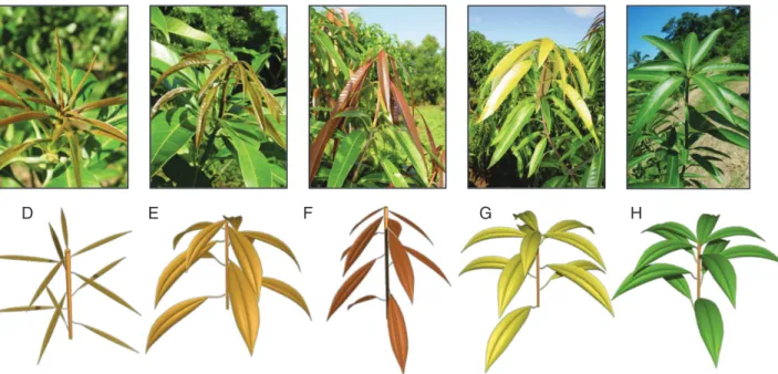
D E F G H
Fig. 1. Observed and simulated phenological stages D (appearance of the axis), E (laminas half-opened starting to hang down), F (laminas totally opened hanging limply), G (leaves becoming rigid and moving upward) and H (mature growth unit) of the mango growth unit (stage nomenclature and top photographs from
leaves; individual leaf length, width and area; internode length; and phyllotaxy. The values of these variables were determined from empirical distributions measured on mature GUs and from relationships evidenced between them. These distributions and relationships were estimated from experimental data (dataset no. 2) and are presented in Table 1. As suggested by Normand et al. (2009) and Dambreville et al. (2013a), the influence of the position of the GU, apical or lateral with respect to the mother GU, and of the position of the mother GU with respect to its own mother GU were considered in the model when statistic-ally relevant.
The first variable estimated by the GU model is the final length of the GU axis. It is of primary importance since other variables, the number of leaves, the final length of the internodes
and basal diameter of the axis at the end of primary growth, are deduced from the GU axis length [Table 1; eqns (1), (2), (5), (6) and (7). The position of the GU and the position of the mother GU influenced GU axis length, leading to three statistically relevant distributions (Table 1). The number of leaves of the GU was calculated from the final GU axis length using a linear relationship whose parameters depended on the GU’s position [Table 1; eqns (1) and (2)]. The individual length of mature leaves followed a Gaussian distribution depending on the GU’s position. It was considered constant among the leaves of a GU, except for the two most distal leaves, which were smaller. Leaf length decrease was 52 % for the most distal leaf and 38 % for the penultimate leaf compared with the mean leaf length of the other leaves of the GU (Dambreville et al., 2013b). The width and area of the leaves can then be determined from their length with the allometric relationships 3 and 4 given in Table 1. The length of the most basal internode, from the base of the GU to the basal leaf, was modelled differently for apical and lat-eral GUs because of the presence of a long basal internode on lateral GUs. It followed a gamma distribution for apical GUs, whereas it was linearly related to the GU axis length for lateral GUs [Table 1; eqn (5)]. Then, the length Lu of the other succes-sive internodes u of the GU decreases more or less regularly from the base to the top of the axis [Table 1; eqn (6)]. This relationship was estimated using data from Goguey-Muethon (1995). The leaf arrangement along the GU axis followed a 2/5 spiral phyllotaxy (Goguey-Muethon, 1995). The basal diam-eter of the GU at the end of primary growth followed a normal distribution whose mean depends on axis length. Using these variables, the structure and the geometry of a mature GU can be precisely defined and represented (Fig. 1H; Supplementary data Information S1).
A similar approach was adopted to build a structure and geometry model for mature inflorescences. The final length of the main axis of inflorescences followed a Gaussian dis-tribution. The number of second-order axes was linearly related to the main axis length [Table 1; eqn (8)]. The length of the second-order axes was modelled with a lin-early decreasing function along the inflorescence main axis [Table 1; eqn (9)].
The fruit growth model proposed by Léchaudel et al. (2005,
2007) simulates fruit fresh mass every day (see below and
Supplementary data Information S2). The shape of growing fruits was modelled as an ellipsoid whose dimensions, length and two diameters were determined from the fresh mass with allometric relationships [Table 1; eqns (10–12)].
Growth and development of growth units and inflorescences. Whereas the previous section focuses on describing mature GUs and inflorescences, in this section we examine how the considered variables changed over time to model growth and development. Growth duration and development of GU axes, leaves and inflorescence axes are strongly affected by tempera-ture (Dambreville et al., 2013b), justifying the use of thermal time models. These models consist of accumulating daily in-crements of development calculated as the difference be-tween mean daily temperature and a base temperature T below which no development occurs. The growth duration or the
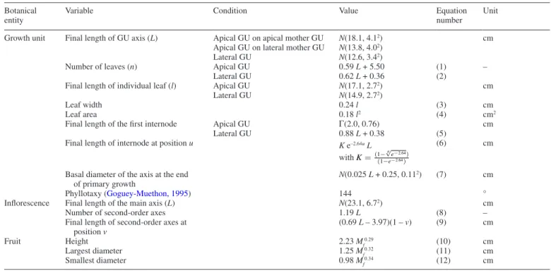
D1 D2 E
F G
gf
Fig. 2. Observed and simulated phenological stages D1 (appearance of the main axis), D2 (bracts begin to fall), E (secondary axis moving away from main axis), F (flowering, from the first to last open flower), G (end of flowering) of the mango inflorescence, and growing fruit (gf) (stage nomenclature and photo-graphs of stages D1–D2–E–F from Dambreville et al., 2015; photographs for
phenological stage is completed when the sum of these daily increments (thermal time sum, tts) reaches a specific threshold TTSS (Arnold, 1959; Bonhomme, 2000). Thermal time models therefore have two parameters, the base temperature T and the thermal time sum threshold TTSS. These parameters were es-timated from dataset no. 2 from Dambreville et al. (2013b) for the main phenological stages of GUs and inflorescences (Table 2), and for the duration of growth of the GU axis, leaf and inflorescence axis (Table 3).
As suggested by Dambreville et al. (2013b), the growth of the GU axis, leaf and inflorescence axis was modelled using a sigmoidal curve (logistic function):
l (tts) = L
1 + e−tts−tipB
(14) where l(tts) is the entity length (cm) at thermal time tts (°Cd), L the final entity length (cm), tip the time of maximum growth rate (inflexion point of the curve, °Cd) and B a slope param-eter (°Cd). Thermal time is counted from bud burst, i.e. pheno-logical stage C for GUs and inflorescences (Figs 1 and 2;
Dambreville et al., 2015). In the modelling process, the final length L of GU axes, leaves and inflorescence axes were de-termined by the previous models of structure and geometry of these organs (Table 1). The growth curve parameters (L, tip and
Table 1. Models for the variables characterizing the structure and geometry of mature growth units (GUs), mature inflorescences and
growing fruits for the mango cultivar Cogshall
Botanical entity
Variable Condition Value Equation
number Unit Growth unit Final length of GU axis (L) Apical GU on apical mother GU N(18.1, 4.12) cm
Apical GU on lateral mother GU N(13.8, 4.02)
Lateral GU N(12.6, 3.42)
Number of leaves (n) Apical GU 0.59 L + 5.50 (1) –
Lateral GU 0.62 L + 0.36 (2)
Final length of individual leaf (l) Apical GU N(17.1, 2.72) cm
Lateral GU N(14.9, 2.72)
Leaf width 0.24 l (3) cm
Leaf area 0.18 l2 (4) cm2
Final length of the first internode Apical GU Γ(2.0, 0.76) cm
Lateral GU 0.88 L + 0.38 (5)
Final length of internode at position u K e–2.64u L with K =(1−√ne−2.64)
(1−e−2.64)
(6) cm
Basal diameter of the axis at the end of primary growth
N(0.025 L + 0.25, 0.112) (7) cm
Phyllotaxy (Goguey-Muethon, 1995) 144 °
Inflorescence Final length of the main axis (L) N(23.1, 6.72) cm
Number of second-order axes 1.19 L (8) –
Final length of second-order axes at
position v (0.69 L – 3.97)(1 – v) (9) cm
Fruit Height 2.23 Mf0.29 (10) cm
Largest diameter 1.25 Mf0.32 (11) cm
Smallest diameter 0.98 Mf0.34 (12) cm
The main variables for growth unit and inflorescence models are the main axis length (L), and the fresh mass (Mf) for the fruit model. Several traits of the growth unit model are conditioned by the apical or lateral position of the growth unit and possibly of its mother growth unit.
N, Gaussian distribution; Γ, Gamma distribution, n, number of internodes of the axis; u, normalized internode position along the main axis of the GU (u is equal to 0 for the second GU axis internode from the base, to 1 for the nth internode at the top, and to i/n for the ith internode from the base); v, normalized position along the main axis of the inflorescence (v is equal to 0 at the base of the inflorescence axis and to 1 at the top).
Table 2. Parameters of the thermal time models for each phenological stage of the growth units and inflorescences for the cultivar
Cogshall
Botanical entity Parameter Phenological stages
D E F G
Growth unit Base temperature T (°C) 13.4 13.4 13.4 9.8
Stage duration TTSS (°Cd) 38.5 47.6 47.4 316.4
Inflorescence Base temperature T (°C) 11.1 8.7 15.1 –
Stage duration TTSS (°Cd) 70.5 133.3 230.4 –
B) and the growth duration (TTSS) were estimated for each GU axis, leaf and inflorescence axis of the database of Dambreville et al. (2013b). Statistical analyses showed that tip could be es-timated as half of the thermal time sum threshold required for growth duration for GU axes and leaves. This result did not hold for inflorescence axes, and the tip value for the inflorescence growth model was estimated as a constant equal to the mean of the estimated tip for each inflorescence. The slope parameter B was calculated from relationships between the maximal abso-lute growth rate at tip and the final length L (Dambreville et al., 2013b). It was constant for the growth models for GU and in-florescence axes, and depended on the final length L for leaves [Table 3; eqn (13)].
The length of the internodes of a GU at a given time tts during growth was determined by applying the ratio between the current (at time tts) and the final length of the GU axis over their final length estimated as in Table 1, and eqns (5) and (6). A similar approach was used for GU diameter, leaf width and length of second-order inflorescence axes.
The GU secondary growth was modelled here using the pipe model theory (see Lehnebach et al., 2018 for a review). On the basis of this theory, a relationship can be established between the diameter d of a given GU and the diameters of its daughter GUs. We generalized it by considering the total number (nbd) of descendant GUs carried by a GU and established the fol-lowing empirical relationship with its diameter d:
d = 0.88 nbd0.41
(15) During a simulation, the diameter d of a GU is updated each time a new descendant GU is produced.
Fruit growth. The fruit growth model simulated the daily in-crease of fresh mass of each individual fruit. The fruit is as-sumed to go through two phases that are considered in the model: the first one corresponds to cell division and the second one to cell expansion. First, a dry mass Md (g) is determined for each fruit at the end of the phase of cell division (352.7 °Cd after full bloom with 16 °C as the base temperature) by sam-pling in an empirical distribution modelled as a mixture of two Gaussian distributions (Léchaudel et al., 2006):
Md∼ 0.97 N 13.9, 4.12 +0.03 N 29.2, 0.662
(16) The corresponding fruit fresh mass Mf (g) is then given by the following allometric equation:
Mf = 23.647 ∗ Md0.6182
(17) Secondly, the fruit growth model simulates growth during the cell expansion phase and determines the fruit fresh mass each day, as well as the final fruit fresh mass at maturity (Léchaudel et al., 2005, 2007). It is based on a mathematical
representation of carbon-related ecophysiological processes (i.e. leaf photosynthesis, mobilization/storage of reserves, res-piration, demand for growth and carbon allocation) occurring at the fruiting branch scale (Léchaudel et al., 2005), and water-related biophysical processes (i.e. water flows driven by stem and fruit water potentials and fruit transpiration) occurring at the fruit scale (Léchaudel et al., 2007). In this model, fruiting branches are assumed to be independent in terms of carbon balance. The model simulates changes in fruit dry and fresh mass at a daily time step, according to hourly weather con-ditions (temperature, relative humidity and light intensity), fruiting branch light environment and leaf to fruit ratio of the fruiting branch. The light environment of each fruiting branch is randomly selected from a set of contrasted environments, characterized by different gap fractions, measured in mango trees. The model also simulates the accumulation of organic compounds (sucrose, fructose, glucose, citric and malic acids) and minerals (K, Mg and Ca) in fruit flesh at a daily time step with empirical relationships between thermal time since full bloom and fruit flesh dry mass. A more detailed descrip-tion of this fruit growth model is given in Supplementary data Information S2.
Graphical representations. To graphically model develop-ment of GUs and inflorescences, specific sets of colours and branching angles for the leaves and second-order inflorescence axes were chosen for the different phenological stages of the GUs and inflorescences, respectively, and were linearly inter-polated according to the development progress within the stage. Inflorescences also undergo a number of transformations. Flower buds were represented as simple spheres until they open. Individual flowers were then represented as simple pol-ygonal meshes during the flowering stage F. Finally, to simulate the bending of the inflorescence axis under fruit mass, a simple gravitropism proportional to fruit fresh mass was applied. As a result, the image sequences depicted in Figs 1 and 2 could be generated.
Model of tree architecture development
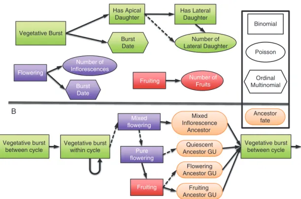
Description of the model of tree architecture development. The individual GUs, inflorescences and fruits, whose growth and development models are described in the previous section, need to be dynamically assembled into a complete architecture. Their appearance is considered at the scale of individual ter-minal GUs and can be decomposed into elementary processes describing the occurrence, intensity and timing of the develop-ment, modelled by binomial, Poisson and ordinal multinomial distributions, respectively (Dambreville et al., 2013a). These processes are assembled to form vegetative burst, flowering and
Table 3: Parameters for the sigmoidal growth models of the growth unit axes, leaves and inflorescence axes Botanical entity Base temperature T (°C) Growth duration TTSS (°Cd) tip (°Cd) B (°Cd)
Growth unit axis 9.2 178.8 89.4 22.4
Leaf 10.7 182.0 91.0 L/(0.06 L–0.08) (13)
Inflorescence axis 11.1 346.0 136.6 50.9
fruiting automata (Fig. 3A). Each automaton is a succession of stochastic processes driven by the value taken by the binomial distributions and determining the occurrence, the number and the appearance date of daughter GUs and inflorescences, and the occurrence of fruiting and number of fruits produced, re-spectively, on each terminal GU. These elementary processes are affected by structural and temporal architectural factors characterizing each terminal GU (Dambreville et al., 2013a). The automata account for these effects by conditioning the stat-istical distributions underlying the processes with these factors (see below).
For vegetative burst, the production of at least one daughter GU is sampled for each terminal GU in a binomial distribution. If the answer is positive, a subsequent binomial distribution tests if there is one apical daughter GU. If not, we assume that all daughter GUs are in a lateral position. If there is an apical daughter GU, the automaton uses a specific binomial distribu-tion to test if there is at least one lateral daughter GU. In the case of the occurrence of lateral daughter GUs, their number is determined with a Poisson distribution. Finally, the burst date of the daughter GUs is simulated with an ordinal multinomial distribution for which the month of bud burst is considered as the response, i.e. one of the 9 months of the vegetative period of the growing cycle. We assumed that all daughter GUs appear
synchronously on a given terminal GU, which is the most common case.
GUs in a terminal position at the end of the vegetative period can potentially flower and set fruit. This is simulated by the flowering and fruiting automata, respectively. For each terminal GU, a binomial distribution tests if flowering occurs. If posi-tive, the number of inflorescences is determined by a Poisson distribution, and the inflorescence(s) burst date (different weeks of the flowering period) is simulated by an ordinal multinomial distribution. Fruit set is then tested on flowering GUs using a binomial distribution. If positive, the number of fruits is sam-pled within a Poisson distribution.
These automata are then combined into the model of tree architecture development, an automaton at a higher level of ab-straction that results from the chaining of the different vege-tative, flowering and fruiting automata between and within growing cycles (Fig. 3B). The model starts at the beginning of the period of vegetative growth of the growing cycle, on the ancestor GUs, i.e. the terminal GUs at the end of the pre-vious growing cycle. The automaton related to vegetative burst (Fig. 3A) is applied to the ancestor GUs to simulate the first layer of GUs during the current growing cycle (vegetative burst between cycles; Fig. 3B). The distinction between vegetative growth between cycles and within a cycle is justified by the
Vegetative burst
within cycle Pure
flowering Mixed flowering Fruiting Vegetative burst between cycle Quiescent Ancestor GU Flowering Ancestor GU Fruiting Ancestor GU Mixed Inflorescence Ancestor Flowering Number of Inflorescences Burst Date Fruiting Number of Fruits Vegetative Burst Has Lateral Daughter Number of Lateral Daughter Burst Date Has Apical Daughter Binomial Poisson Ordinal Multinomial Ancestor fate Vegetative burst between cycle A B
Fig. 3. Stochastic automaton applied to each terminal growth unit (GU) to simulate the development of mango tree architecture and mango fruit production as directed graphs with nodes representing the different elementary developmental processes. The shape of each frame indicates the distribution underlying each de-velopmental process or the ancestor fate entity in the case of pill-shaped frames. The edges indicate the succession of the processes. Their shape indicates that the succession is conditioned by a positive (solid arrow) or negative (dashed arrow) value of the realization of the parent binomial process. The three upper diagrams (inspired from Dambreville et al., 2013a) represent vegetative (green automaton), flowering (purple automaton) and fruiting (red automaton) developments (A).
fact that the ancestor GU is characterized by specific factors, in particular its fate, which affect its behaviour as a mother GU (Dambreville et al., 2013a). The fate of the ancestor GU can be quiescent if the ancestor GU did not flower during the previous cycle, flowering if it flowered and did not set fruit, or fruiting if it flowered and set fruit. In this study, the factors that are con-sidered to affect processes of vegetative burst between cycles are ancestor GU fate, date of burst and position. To initiate the simulation for each ancestor GU, values of these factors could be recorded on an actual tree, could be randomly sampled in empirical distributions or could result from the simulation of previous cycles (see below).
The automaton of vegetative burst is then applied on the GUs generated by the previous step (vegetative burst within a cycle,
Fig. 3B). Factors considered to affect processes of vegetative burst within a cycle are mother GU position and date of burst, and ancestor GU position and fate.
When no vegetative burst occurs on a terminal GU during the vegetative growth period of a cycle, this GU is in the terminal position during the flowering period and is then susceptible to flower and set fruit (it becomes an ancestor GU for the fol-lowing growing cycle). The model first tests if the GU produces mixed or pure inflorescences. We assume that only one type of inflorescence (mixed or pure) appears on a given GU. Using a binomial distribution, we first test if mixed inflorescences are produced. In the positive case, the number and the date of appearance of inflorescences are determined with a flowering automaton calibrated for mixed inflorescences. In the negative case, pure inflorescences are tested with a corresponding au-tomaton. In the case of a pure inflorescence, the model then tests if the GU sets fruits with another binomial distribution. The fruiting automaton is then applied to simulate the number of fruits. In this study, the factors considered to affect the re-productive development processes are the position and the date of burst of the mother GU, and the fate and position of the an-cestor GU of the previous cycle. The result of these simulations defines the fate of each ancestor GU for the simulation of vege-tative growth during the following cycle (Fig. 3B). At the tree scale, the results of these simulations are used to calculate vari-ables such as flowering rate, fruiting rate or fruit production.
Once the number of daughter botanical entities (GU, inflor-escence, mixed inflorescence) and their burst date are simulated for each GU, buds representing these organs are positioned at the distal end of the GU axis, according to the phyllotactic angle of 144° with a branching angle of 60°. Fruits are distrib-uted on the inflorescences of the fruiting GUs.
Model parameterization. Parameters of processes of the au-tomata were estimated individually on the basis of three meas-ured Cogshall mango tree architectures presented in Dambreville et al. (2013a). In this context, vegetative growth occurs from September to May, flowering from July to September, and har-vest from December to February. The database was converted into the MTG format (Godin and Caraglio, 1998). A Python script extracted the different GUs and the information related to their vegetative and reproductive development from this struc-tural database. The resulting table was processed using R (R Core Team, 2016). The effects of the temporal and structural factors were tested with generalized linear models (GLMs), using the glm function for the binomial and Poisson responses,
and the vglm function of the VGAM package (Yee, 2015) for the ordinal multinomial responses (Fig. 3). Significant factors were selected based on the Akaike information criterion (AIC) using the step function for the binomial and Poisson responses, and a specifically implemented function for the ordinal multi-nomial responses. Finally, the predict.glm and predict.vglm functions calculated the predicted probabilities for each com-bination of modalities of the significant factors. For each GLM, significant first-order interactions were integrated after the selection of the significant explanatory factors and were thus taken into account in the predicted probabilities estimation. All the probability tables were saved and used for the simulations.
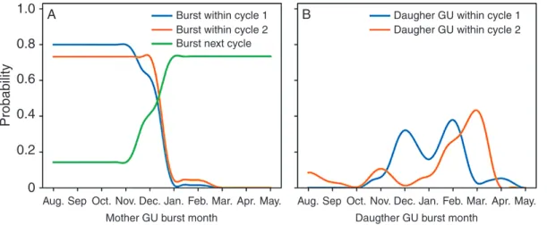
The probability tables determined with this parameterization method from empirical data highlighted several results that are pre-sented below. For GU production within a growing cycle, GUs that burst from August to December had a high probability (P = 0.80) to produce daughter GUs within the same growing cycle, while those that burst later in the cycle had a low probability (P = 0.02) (Fig. 4A). As a result, GUs that appeared after December tended to produce their daughter GUs during the next cycle (P = 0.73).
GUs that produced daughter GUs within the same cycle had a high probability to produce an apical daughter GU (P = 0.98). Apical mother GUs had a higher probability to produce lateral daughter GUs (P = 0.66) than lateral mother GUs (P = 0.28) and, when they did, apical mother GUs produced a higher number of lateral daughter GUs than lateral mother GUs (on average, 2.1 vs. 1.3 for cycle 1, and 2.3 vs. 1.9 for cycle 2), in accordance with Normand et al. (2009).
During cycle 1, successive daughter GUs appeared with a regular pattern, on average 2.2 months after the burst date of the parent GUs, leading to regular peaks of GU production in December, February and April (Fig. 4B). During cycle 2 (Fig. 4B), the average delay between successive GU burst dates was about 3.0 months, leading to peaks of GU production in August, November and February/March. However, GU produc-tion was low from flowering to harvest (August to January) and high after harvest in February/March.
The production of GUs between growing cycles was strongly affected by the fate of the ancestor GUs. Only quiescent an-cestor GUs could produce an apical daughter GU during the next growing cycle (P = 0.82) since the apical bud was trans-formed into an inflorescence for flowering and fruiting ancestor GUs. The probability of producing lateral daughter GUs for quiescent ancestor GUs was P = 0.46. The mean number of lateral daughter GUs depended on the fate and position of the ancestor GU. The flowering and fruiting ancestor GUs pro-duced more lateral daughter GUs (3.4 and 4.2, respectively) than quiescent ancestor GUs (2.4), probably due to the loss of apical dominance with apical flowering (Normand et al., 2009;
Capelli et al., 2016).
The fate of the ancestor GU also affected the timing of burst in the following cycle. Quiescent ancestor GUs tended to pro-duce daughter and descendant GUs during the following cycle according to a 3 month pattern, depending on the ancestor GU burst date (Fig. 5A). Flowering (Fig. 5B) and fruiting (Fig. 5C) ancestor GUs produced daughter and descendant GUs mainly or only, respectively, after fruit production, and the ancestor GU burst date did not affect this pattern for fruiting ancestor GUs.
Mixed inflorescences were produced with a very low prob-ability (P = 0.06) and mainly on terminal GUs generated
between January and March. They were always the only inflor-escence, located in the apical position. Mixed inflorescences themselves had a probability P = 0.53 to produce at least one daughter GU. They produced an average of 2.3 daughter GUs, and the probability that one of them was in the apical position was P = 0.47. Daughter GUs appeared on these mixed inflores-cences between December and February.
Pure inflorescences were mainly produced by terminal GUs generated between October and May. The probability of flowering was positively affected by the apical position of the terminal GUs and by the non-fruiting fate of the ancestor GUs of the previous cycle (long-term effect of the ancestor GU fate). The number of inflorescences produced per terminal GU was usually one, except for GUs generated in December–January that produced an average of 1.6 inflorescences. The date of flowering of the inflorescences was recorded only during cycle 2, and most of the GUs flowered in September according to a two-peak pattern.
The fruiting probability was estimated at the terminal GU scale and not at the inflorescence scale. The date of flowering
of the inflorescences affected the GU fruiting probability. The earlier the inflorescences flowered, the higher the GU fruiting probability was. The fruiting probability was P = 0.40 on average for GUs whose inflorescences flowered between July and 15 September, P = 0.20 for those whose inflorescences flowered from 15 September to 15 October, and 0 for those whose inflorescences flowered after 1 October. Apical GUs had a higher fruiting probability than lateral GUs. The number of fruits generated by a GU was positively related to the number of inflorescences of that GU.
Model implementation. The implementation of the simula-tion model for plant architectural development was carried out using the L-Py module (Boudon et al., 2012) of the OpenAlea platform (Pradal et al., 2008) that mixes the formalism of L-systems (Prusinkiewicz, 1990) and the Python language. Simulations of the development and visual representation of the structure and its organs were thus formalized as L-system rules with the Python code. Rules related to the architectural sub-model are responsible for the creation of new botanical entities. Once created in the architecture, rules of the GU and
1.0 Burst within cycle 1
Burst within cycle 2
Daugher GU within cycle 1 Daugher GU within cycle 2 Burst next cycle
A B
0.8
Aug. Sep Oct. Nov. Dec.
Mother GU burst month
Jan. Feb. Mar. Apr. May. Aug. Sep Oct. Nov. Dec.
Daugther GU burst month
Jan. Feb. Mar. Apr. May.
0.6
Probability 0.4
0.2 0
Fig. 4. (A) Probability that a mother growth unit (GU) produces at least one daughter GU within the same cycle or during the following cycle (vegetative burst between cycles 1 and 2) according to its burst month. (B) Probability of appearance of daughter GUs for each month during cycles 1 and 2. These probabilities
were inferred from measured development of three mango trees.
1.0
Quiescent ancestor GU Flowering ancestor GU Fruiting ancestor GU
Mother from previous cycle Mother from August–October Mother from November Mother from December– February
Jul. Aug. Sep. Oct. Nov.
Daughter GU burst month-cycle 2 Daughter GU burst month-cycle 2 Daughter GU burst month-cycle 2 Dec. Jan. Feb. Mar. Apr. Jul. Aug. Sep. Oct. Nov. Dec. Jan. Feb. Mar. Apr. Jul. Aug. Sep. Oct. Nov. Dec. Jan. Feb. Mar. Apr.
A B C 0.8 0.6 Probability 0.4 0.2 0
Fig. 5. Monthly probability of the appearance of daughter growth units (GUs) during cycle 2 according to the burst month of the mother GU and the fate of the ancestor GU of cycle 1 [quiescent (A), flowering (B) or fruiting (C)]. The blue line represents direct daughter GUs of ancestor GUs (between-cycle production), and orange, green and red lines represent daughter GUs of mother GUs produced within the growing cycle (within-cycle production) during the periods of August
inflorescence sub-models infer the attributes of the entities and simulate their development. The sub-model that formalizes fruit growth was developed with the R software (Léchaudel et al., 2005). Communication between the main model in Python and this R sub-model was performed using file exchange or via the RPy 2 module. The main model provides parameters to the fruit growth sub-model such as the bloom date of the inflorescences and the number of leaves and fruits of the GUs belonging to the fruiting branches. In return, the sub-model provides the es-timated dynamic of the fruits in term of fresh mass and organic compounds.
Finally, running the model makes it possible to achieve visual results such as those depicted in Fig. 6 and in Supplementary data Video S1.
MODEL EVALUATION
The V-Mango model presented herein brings together nu-merous sub-models that act as local rules and are assembled as described above. It appears important therefore to evaluate how the model behaves as a complex assembly of components estimated individually. In order to perform this evaluation, we compared simulated data with data used for the param-eterization at a global scale of a set of three trees during two growing cycles (dataset no. 1). The influence of structural and
temporal factors on the architectural development and, conse-quently, their relevance to condition model probabilities was then quantified.
Assessment of the global quality of the simulations
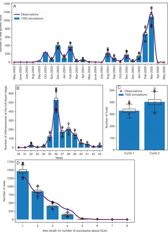
We used four global structural and temporal criteria, Ci i∊ [1,4], that were relevant to the objectives of the model, to evaluate the consistency of the assembly of the model components (Fig. 3). To assess the size and the dynamics of the population of botanical entities, we considered as global criteria the demography of the GUs (C1) and the demog-raphy of the inflorescences (C2), corresponding, respect-ively, to the number of GUs that burst each month and the number of inflorescences that bloomed each week during a simulated period. The criterion for fruit production (C3) was the total number of fruits produced per growing cycle. The fourth criterion was the distribution of axes lengths at the end of the two growing cycles (C4), a characteristic re-lated to the organization of the generated architecture. In this case, an axis begins with a lateral GU and is formed by the successive apical GUs. The metrics is the number of GUs. We considered only the GUs that appeared during the simulated period.
Fig. 6. Stochastic simulation of the architecture of a mango tree at different periods of the growing cycle. From left to right and top to bottom, the initial struc-ture, a flush of growth units during the period of vegetative growth (young extending leaves are in yellow), the flowering period with inflorescences and the fruit
These global structural and temporal criteria were computed on a set of three simulated trees and were compared with the values computed on a set of three actual trees. The starting point for simulations was the three trees described at the be-ginning of the first studied growing cycle. Their terminal GUs
(=ancestor GUs) were individually characterized by their pos-ition and their fate. Vegetative growth, flowering, fruiting and fruit production were simulated during two successive growing cycles. One thousand simulations were performed and the four criteria Ci were computed for each simulation.
1400 A Observations 1000 simulations 1200 1000 800 Number of ne w gro wth units 600 Ma y-2003
June-2003 July-2003 Aug-2003 Sep-2003 Oct-2003 No
v-2003
Dec-2003 Jan-2004 Feb-2004 Mar-2004 Apr-2004 May-2004 June-2004 July-2004 Aug-2004 Sep-2004 Oct-2004 No
v-2004
Dec-2004 Jan-2005 Feb-2005 Mar-2005 Apr-2005 May-2005
600 500 400 300 200
Number of inflorescences at the full
bl oom stag e Number of fr uits Number of ax es 100 1750 Observations 1000 simulations D B C 1250 1000 750 500 250 1 2 3 4
Axis length (in number of successive apical GUs)
5 6 7 8 0 1500 30 31 32 33 34 35 36 37 Week 38 39 40 41 42 43 0 500 400 300 200 100 Cycle 1 Cycle 2 0 400 200 0
Fig. 7. Global characterization of model simulation, with the blue histogram and boxplots representing, respectively, the average and distribution of 1000 simu-lations of three mango trees during two growing cycles. The purple lines and points are the actual values for the three measured mango trees. (A) The monthly demography of growth units (GUs) for growing cycles 1 and 2; (B) the weekly demography of inflorescences at the full bloom stage for the flowering period of
The results obtained for these four global criteria were in good visual agreement with the measured values (Fig. 7), the actual data being in the range of the simulated data. To assess this, we first computed an average value for each criterion from the 1000 simulations, thus representing an ‘average simulation’. For the GU demography, for instance, we computed the mean number of GUs generated each month from the 1000 simula-tions, resulting in a monthly mean number of GUs that appeared on the three trees during the two simulated growing cycles.
To test if the actual and the average simulated distributions were drawn from the same distribution, we performed a χ 2 test
for each criterion. The P-values of the test for the demography of GUs and inflorescences were P = 0.24 and P = 0.23, respect-ively. It was P = 0.19 for the number of fruits produced and P = 0.22 for the axis length criteria. The hypothesis of dissimi-larity was thus rejected, confirming the consistency between the actual and the average simulated distributions.
To characterize the error made by the simulations on each global criterion, we computed the root mean square error (RMSE) on the simulated values of each global criterion. RMSE for the criterion Ci was computed in the following way:
RMSEi(M, R) = … 1 n n k=1(r i k− vik)2 (18) where ri
k is the k-th component of the value for the criterion Ci
estimated on the actual data R, and vi
k is the average value of the
k-th component of Ci computed from 1000 simulations with the model M. In order to compare criteria, we normalized the root mean square error (NRMSE):
NRMSEi(M, R) = RMSEi(M, R)
(ri
max− rmini )
(19) where ri
min and rimax are the minimum and maximum values of
Ci for the measured data R, respectively.
In our simulations, NRMSE was about 3 % for the GUs and inflorescence demography, 4 % for the number of fruits and 7 % for axis length. This showed the good ability of the model to reproduce structures and dynamics similar to the actual ones.
Influence of temporal and structural factors in architectural development
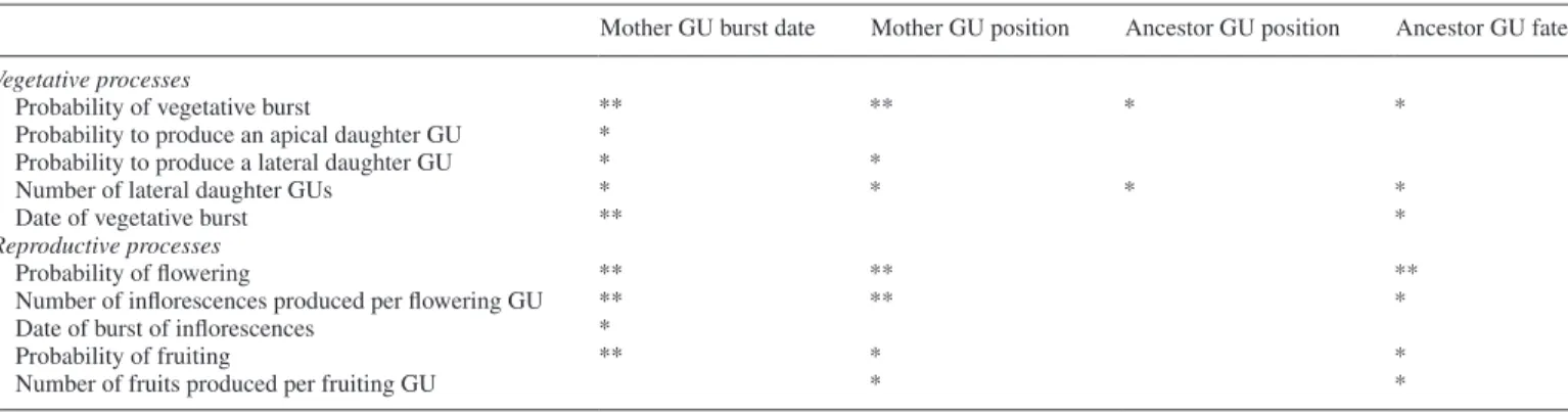
Similar to Dambreville et al. (2013a), the factors with a sig-nificant influence on each individual developmental process at the GU scale were identified using GLMs for each growing cycle (Table 4), and probability tables for each process in the model were determined accordingly. In a second step, a com-plementary analysis was conducted at the tree scale to quanti-tatively assess the influence of each factor on the simulation of the entire architectural development of a set of three trees. By comparing the analysis at the two scales, a better overview of the influence of the different factors could be assessed.
Characterization of the influence of the structural and temporal factors at the GU scale. The significant structural and temporal factors for the different vegetative and reproductive processes are presented in Table 4. The burst date of the mother GU had a significant effect on all vegetative and reproductive processes, except the number of fruits produced per fruiting GU. The pos-ition of the mother GU and the fate of the ancestor GU also had a significant influence on most of the vegetative and repro-ductive processes. The influence of the ancestor GU position was limited to two vegetative processes (probability of vegeta-tive burst and number of lateral daughter GUs).
However, since the number of processes in the model was high, with complex interdependencies, and the magnitude of the effect of each factor on the different processes varied consider-ably, it was not possible to assess the influence of each structural and temporal factor on the simulations at the tree scale with the complete model from these results at the GU scale.
Characterization of the influence of the structural and temporal factors at the tree scale. To quantitatively assess the influence of each structural and temporal factor on the architectural de-velopment at the tree scale, we used the following methodology. First, a set of four new models was built, with each model Mj, j∊ [1,4], corresponding to the complete model Mc presented above without one of the structural or temporal factors Fj in the model parameterization. A null model M0 was also built without
Table 4. Influence of the temporal and structural architectural factors (columns) on individual processes of vegetative and reproductive
development at the growth unit (GU) scale (rows)
Mother GU burst date Mother GU position Ancestor GU position Ancestor GU fate
Vegetative processes
Probability of vegetative burst ** ** * *
Probability to produce an apical daughter GU *
Probability to produce a lateral daughter GU * *
Number of lateral daughter GUs * * * *
Date of vegetative burst ** *
Reproductive processes
Probability of flowering ** ** **
Number of inflorescences produced per flowering GU ** ** *
Date of burst of inflorescences *
Probability of fruiting ** * *
Number of fruits produced per fruiting GU * *
**The factor has a significant effect (P-value <0.01) on a process during both cycles and during transitions between cycles; its influence is considered as global. *The significant effect of the factor depends on the cycle and/or on the transition between cycles; its influence is considered as partial. No *, the factor has no effect on the process.
any factor. We then defined the influence index I(Ci, Fj), with i∊ [1,4] and j∊ [1,4], to measure the influence of a factor Fj on the global criteria Ci:
I (Ci, Fj) = NRMSEi(Mj, Mc)
NRMSEi(M0, Mc)
(20) The numerator represents the error made on the global criteria Ci by the simulations of a model Mj which did not consider the factor Fj, compared with the error made by the complete model, thus giving a value for the benefit of taking into account the factor Fj in the complete model. To make the index compar-able between all the criteria, the numerator was normalized by the NRMSE of the null model M0 compared with the complete model Mc for each criterion. One thousand simulations of a set of three trees were made to compute each index I(Ci, Fj).
A value of the index I(Ci, Fj) between 0 and 1 was expected, indicating the contribution of the factor Fj to the improvement of the simulations between the null model M0 and the complete model Mc. The closer to 1 the index value was, the greater the contribution of the factor Fj was. A value above 1 indicated that the error made by model Mj was higher than that of the null model M0, and, thus, that considering only the factors other than Fj disrupted the simulation. The case I(Ci, Fj) >1 therefore confirmed the great importance of the factor Fj for controlling the structure and the temporality in the simulation.
The computed indexes I(Ci, Fj) are given in Table 5. The re-sults showed that for the three global criteria related to the number and the temporality of the botanical entities in the struc-ture (GU demography, inflorescence demography and number of fruits produced), a strong effect of mother GU burst date was ob-served, with influence indexes >1. The ancestor GU fate ranked second for its influence in the model. The other two factors seemed to have marginal effects on these three global criteria. For the fourth global criterion, axis length, related to the ar-rangement of the botanical entities, the mother GU position and burst date were the most important factors, with similar values of the influence index. The ancestor GU fate had an influence index value similar to the one it had for the three other criteria.
APPLICATIONS OF THE MODEL
Two examples of model applications are illustrated in this section. First, we show how a time series of susceptibility to pests can be estimated from the phenological modelling of each individual botanical entity of the tree. Secondly, we use an in-verse modelling approach to determine the adequate size of fruiting branches to enable optimal fruit growth by comparing fruit size simulated by the model with different fruiting branch
sizes with the actual fruit size. We thus assess their level of physiological autonomy (Sprugel, 1991) with regard to carbon supply to the fruit, which is a main aspect of fruit production sustainability (Lauri and Corelli-Grappadelli, 2014).
Changes in tree phenology over time
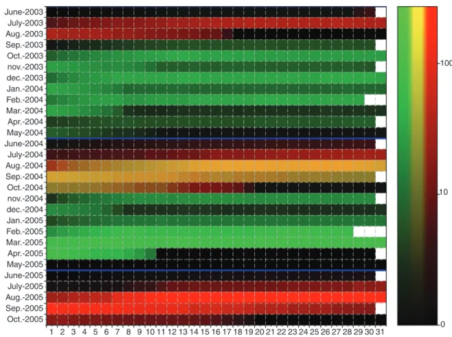
Coupling of developmental models at the scale of the whole tree and at the scale of the individual botanical entities made it possible to precisely quantify the demography of the dif-ferent phenological stages present at each date in a tree or an orchard. As an illustration, we estimated the daily number of GUs or inflorescences at the phenological stages D or E (Figs 1
and 2) during the two growing cycles of the simulation. These stages are known to be critical because GUs and particularly inflorescences at these stages are susceptible to the mango blossom gall midge, Procontarinia mangiferae (Felt) (Diptera: Cecidomyiidae), a pest of economic importance (Amouroux et al., 2013). The model was run on a virtual orchard of 100 trees, each tree being randomly sampled within the three meas-ured tree architectures. For each day of the two growing cycles, the number of GUs and inflorescences in the trees at pheno-logical stages D or E were counted (Fig. 8). To improve visual-ization, these numbers were divided by the number of trees and thus give an average number of organs per tree.
The different peaks of production of the GUs and inflores-cences are clearly identifiable on this diagram. For instance, the regular peaks of GU production in October and December 2003, February, August and November 2004, and February and March 2005 are visible, as well as the peaks of inflores-cence production in July–September of each year. Concomitant production of GUs and inflorescences occurred in August and September 2004. In contrast, the periods without phenological stages susceptible to mango blossom gall midge, in general in May and June (in black in Fig. 8), illustrate the resting periods for the trees.
Such time series of susceptibility intensity can be a tool to study the interactions between pests and the mango orchard, and to optimize pesticide treatments or explore the effects of climate change scenarios on the susceptibility of an orchard to pests and diseases.
Autonomy of fruiting branches
As a second application of our model, we explore the re-sults from the coupling of the architectural model to the ecophysiological fruit growth model. This latter fruit model
Table 5. Values of the influence index I(Ci, Fj) expressing the effect of each of the four temporal and structural architectural factors Fj
(columns) used to condition the probabilities of the model of architectural development on the four global criteria Ci (rows) used to as-sess model simulation quality
Global criteria Mother GU burst date Mother GU position Ancestor GU position Ancestor GU fate
Growth unit (GU) demography 1.23 0.06 0.02 0.34
Inflorescence demography 1.46 0.11 0.10 0.18
Number of fruits produced 1.45 0.07 0.01 0.24
was originally used to evaluate the effects of the local leaf:fruit ratio, i.e. the respective size of carbohydrate sources and sinks during fruit growth at the branch level, on individual fruit mass at harvest. Fruiting branch autonomy for carbohydrates might depend on the size of fruiting branches, which defines the number of leaves and fruits and is therefore an important par-ameter (Léchaudel et al., 2005). The objective of this model ap-plication was to assess the level of autonomy for carbohydrates of fruiting branches of different sizes in the mango tree.
We first designed a parametric method to identify the fruiting branches in the simulated architectures. A fruiting branch of size N is defined as the set of GUs located at a max-imal distance in the structure of N GUs from a fruiting GU. Considering the architecture as a tree graph of connected bo-tanical entities (Godin and Caraglio, 1998), the distance be-tween two entities is defined as the number of GUs making up the shortest path linking the two entities in the graph. This size N is a parameter of the model that can be controlled by the user. Practically, each fruiting GU was identified in the structure, and all the GUs that were at a maximal distance in the structure of N GUs from a fruiting GU belonged to the corresponding fruiting branch. If the sets of GUs of different fruiting branches overlapped, they were merged to form a unique fruiting branch with several competing fruiting GUs.
Figure 9A illustrates how fruiting branches are distributed in the tree crown for different size N. With increasing branch
size, GUs of the smallest fruiting branches are merged into fruiting branches of bigger sizes.
A sensitivity analysis of the effects of fruiting branch size N on the average fruit fresh mass at harvest was performed by testing small (N = 1, representing only the fruiting GUs) to large (N = 7 representing the scaffolds) fruiting branches. To make the results comparable, we fixed the development of the archi-tecture by exactly reproducing the development of the meas-ured trees. In this way, the number and timing of appearance of the organs were always the same. However, the morphology of the GUs, in particular, their number of leaves, was variable, simulated by the stochastic GU development model. Two suc-cessive growing cycles are considered. One thousand simula-tions with different random seeds were performed for each of the three measured trees. For each simulation, fruiting branches were identified and their leaf:fruit ratio was determined and used as input parameters in the fruit growth model to modulate carbohydrate acquisition from photosynthesis and partitioning between fruits according to their demand. The carbohydrate reserve in the fruiting branch at the beginning of fruit growth had a fixed value, independent of the fruiting branch size, taken from Léchaudel et al. (2005).
As a result, the leaf:fruit ratio linearly increased with the size of fruiting branches (Fig. 9B), ranging from ten to 90 leaves per fruit. However, the relationship between mean fruit fresh mass at harvest and fruiting branch size followed a sigmoidal
June-2003 July-2003 Aug.-2003 Sep.-2003 Oct.-2003 nov.-2003 dec.-2003 Jan.-2004 Feb.-2004 Mar.-2004 Apr.-2004 May-2004 June-2004 July-2004 Aug.-2004 Sep.-2004 Oct.-2004 nov.-2004 dec.-2004 Jan.-2005 Feb.-2005 Mar.-2005 Apr.-2005 May-2005 June-2005 July-2005 Aug.-2005 Sep.-2005 Oct.-2005 1 2 3 4 5 6 7 8 9 10 11 12 13 14 15 16 17 18 19 20 21 22 23 24 25 26 27 28 29 30 31 0 10 100
Fig. 8. Daily simulated number of growth units (GUs, green channel), inflorescences (red channel) or both (in yellow) at phenological stage D or E per tree during two growing cycles. Months are in rows and days in columns. Data were computed from 100 simulated mango trees. Black colour indicates that no GU or inflorescence at stage D or E is simulated that day. The intensity is represented in log scale. Blue lines indicate the transition between two growing cycles (June).
pattern (Fig. 9C) with an asymptotic value of approx. 440 g during both cycles. The mean measured fruit fresh mass (390 g and 374 g for cycle 1 and 2, respectively) corresponded to the average fresh mass simulated with fruiting branches of size comprised between N = 2 and N = 3. This suggested a local effect of the architecture on fruit growth and, consequently, a relatively good autonomy for carbohydrates of the fruiting branches above size N = 3. This size of the fruiting branches is thus used in the model for subsequent simulations.
DISCUSSION
We presented an FSPM of the architectural development and fruit production of the mango tree. At the GU scale, it is formal-ized as a stochastic automaton that decomposes the vegetative and reproductive development of the architecture into elemen-tary processes modelled with probabilities estimated from ac-tual trees using GLMs.
GLMs provide a flexible modelling of developmental processes From a methodological point of view, stochastic modelling of elementary developmental processes is flexible since it al-lows response variables following various distributions, i.e. binomial, Poisson and ordinal multinomial processes, in our model to represent occurrence, intensity and timing of a pro-cess, respectively. The distributions can be conditioned by various factors affecting the processes, after estimation with GLMs. These processes can then be assembled in a stochastic automaton representing a complex developmental model. This integrative approach that aims at modelling chains of causation in developmental processes is related to the approach of Pearl (2009). Thanks to the flexibility of the approach, the model of architectural development and fruit production can be enriched by taking other significant factors such as environmental con-ditions or cultivation practices into account, or by integrating other processes such as the death of botanical entities (Lauri, 2009). As a limit, however, increasing the number of factors
80 B A 1. 2. 3. 4. 5. 6 C 60 40 Number of le av es per fr ui t Mean fr uit weight (g ) 20 500 450 400 350 300 Cycle 1 Cycle 2 Measured Size : 1 Size : 2 Size : 3 Size : 4 Size : 5 Size : 6 Size : 7
Fig. 9. Testing the effects of different fruiting branch size on fruit growth. A fruiting branch of size N is defined as the set of GUs located at a maximal distance in the structure of N GUs from a fruiting GU. (A) Top views of a mango tree with fruiting branches of size 1–6. Different colours are used to identify the different fruiting branches. Non-fruiting inflorescences are in grey and growth units of non-fruiting branches are in black. (B) Distribution of the computed leaf:fruit ratio for each size of the fruiting branches during each simulated cycle. The leaf:fruit ratio is a main parameter controlling fruit growth. (C) The average fruit fresh mass simulated with different fruiting branch sizes compared with the measured ones (grey lines) during each simulated cycle. For graphs (B) and (C), boxplots