)28 1414
oW\-
2
^
Dewey
WORKING
PAPER
ALFRED
P.SLOAN
SCHOOL
OF
MANAGEMENT
Advertising arid Entry Deterrence:
An Exploratory Model by Richard Schmalensee WP 1309-82 May 1982
MASSACHUSETTS
INSTITUTE
OF
TECHNOLOGY
50MEMORIAL
DRIVE
CAMBRIDGE,
MASSACHUSETTS
02139Advertising and Entry Deterrence;
An Exploratory Model
by
Richard Schmalensee
M.l.i. i_:ar,:-..
JUL
2
9 1-'^"^Advertising and Entry Deterrence: An Exploratory Model
Richard Schmalensee Sloan School of Management
Massachusetts Institute of Technology
ABSTRACT
In this model, the effects of advertising are infinitely durable, fixed (and sunk) costs give rise
to economies of scale, post-entry behavior is non-cooperative, and pre-entry expectations are rational. Despite the obvious resemblance to work on the use of
investment in production capacity to deter entry, here
the incumbent monopolist never finds it optimal to advertise more if entry is possible than if it is not.
This result and other features of this model indicate the dangers of analyzing advertising by analogy with other sorts of Investments. Our results make clear the need for more theoretical work on advertising
and entry deterrence.
May, 1982
(1)
A basic defect in the classic Bain/Sylos limit-pricing model of entry deterrence stems from its assumption that the potential entrant believes that the established firm would maintain its output constant if entry occurred. The problem is that if entry did occur, it would not generally be rational for the established firm to carry out this threat; thus the threat is not credible."•
Recent work on entry deterrence has begun to
correct this defect by exploring the consequences of ruling out such irrational post-entry behavior and of assuming that potential entrants have rational expectations.^ A leading result in that literature is
that in the presence of economies of scale, an established monopoly facing the threat of entry might find it possible and optimal to deter that entry credibly by Investing more in durable production capacity than
it would if no such threat were present.^ Both the durability of the investment and the presence of economies of scale are apparently necessary for this result.
It is generally acknowledged that the effects of advertising persist
over time, and it is often argued that there are important economies of scale in advertising.^ Reasoning by analogy with investment in
production capacity, as is commonly done in this context, one might conjecture (as I did initially) that in any plausible model assuming
durability and scale economies, it will sometimes be optimal for an
established monopolist to over-advertise in order to deter entry credibly. Baldani and Masson (1981) have recently built a model which is
consistent with this conjecture. Their over-advertising result seems a
bit forced, however, since under their assumptions a monopolist protected
from entry would spend nothing at all on advertising. If the incumbent advertises in advance of entry, it is assumed to create durable
"goodwill" that forces the entrant to advertise in order to sell
(2)
sales at all advertising levels. If entry does not occur, the
incumbent's "goodwill" is assumed not to affect its demand. The assumed properties of "goodwill" are not related to a model of Individual buyer behavior, and post-entry equilibrium is not fully modeled.
This essay presents an alternative model, patterned on those focusing on investment in production capacity and constructed to explore the role of advertising in entry deterrence. Though the assumptions made here
have a superficial resemblance to those of Baldani and Masson (1981), our
results are quite different. In this model, the effects of advertising
are infinitely durable, fixed costs give rise to economies of scale, post-entry behavior is noncooperative, and pre-entry expectations are
rational. Yet the incumbent monopoly never finds it optimal to advertise
more if entry is possible than if it is not. Optimal entry deterrence always involves advertising less than if the threat of entry were
absent. Certain disadvantages of size appear in this model's post-entry
equilibria, and it may be better to enter second than first. These results and others presented below make plain the dangers of analyzing
investments in advertising largely by analogy with investments in
production capacity. They also suggest that the strategic implications
of investments in advertising may be highly sensitive to the effects of
advertising on buyer behavior and to the nature of post-entry equilibrium.
I. Assumptions
We deal throughout with only two firms, X and Y. Perhaps because of stochastic factors in the product development process, firm X appears on the market first. When firm Y subsequently appears, it may or may not
(3)
elect to enter. Both firms produce the same product If they produce anything.
There is a continuum of potential buyers with linear individual
demand curves. The total mass of these buyers is normalized to be unity for convenience, and the units in which prices and quantities are
measured are chosen so that if a fraction e of potential buyers are
aware of the product, their total demand is given by
q = 9(1 - p), or p = 1 - (q/e),
(D
where p is the market price and q is the total quantity demanded. The
unit cost of production, y» is a constant less than one for both
firms. None of what follows seems to depend critically on demand linearity or cost constancy.
In order to make any sales, firm X must invest a fixed amount, f, to design leaflets and prepare to print them. This cost is forever
sunk.^ It then prints leaflets and sends them at random to potential
buyers, exactly as in Butters (1977). There is a constant printing and
distribution cost per leaflet sent. Buyers who receive one or more leaflets are aware forever of X's location and the attributes of its
product. Those who receive no leaflets never learn about this product. The effects of this introductory advertising are thus infinitely
durable. Butters (1977) notes that if L leaflets are sent at random to B buyers, and both L and B are large, then the fraction of buyers informed
is approximately equal to [1 - exp(-L/B)]. Treating this fraction as
exact, and letting a equal B times the printing and distribution cost of
a single leaflet, we obtain the cost of informing a fraction x of potential buyers:
(A)
cCx) = f - a InCl - x). (2)
We will use x for the fraction informed by firm X and y for the fraction
informed by firm Y, which faces the same advertising cost function. Note
that (2) implies a U-shaped average cost function for real advertising,
X. Much of what follows holds for all cost functions of this sort. We begin by analyzing firm X's behavior if subsequent entry Y is
impossible. Section III describes post-advertising noncooperative
duopoly equilibria, treating x and y as exogenous. Basic properties of
the profit functions generated by these equilibria are shown in Sections IV and V to produce non-standard reaction functions in (x,y) space and to drive the results on entry deterrence described above.
II. Monopoly Equilibrium
Suppose that X has just informed x potential buyers with its initial
introductory advertising and subsequent entry is impossible. Then X will optimally maintain its price and quantity constant forever. The present value of its net revenue is
tt(x) = x(l - p)(p - Y)/r = q[(l - q/x) - yl/r, (3)
where r is the relevant discount rate, and p and q are price and
quantity, respectively. If q is chosen optimally, price, quantity, and
present value are given by
p» = (1 + y)/2, q* = x(l - p*) = x(l - y)/2, tt^(x)
= x(l - Y)^/Ar,
respectively. It will simplify formulae in what follows to work with re-scaled profits, II^(x) = rTr'"(x)/(l - y)^ = x/A,
(5)
Taking into account the cost of introductory advertising, X's present value is equal to tt"'(x) minus the cost of advertising:
w^'Cx) = Ti^(x) - c(x) = x(l - Y)^/^r + a ln(l - x) - f
.
2 2
It will be convenient to define A = ar/(l - y) , f" = fr/(l - y) , and C(x) = c(x)r/(l - y)^, and to work instead with
W'"(x) = II™(x) - C(x) = x/4 +
Alnd
- x) - F. (5)Conditional on having prepared to print leaflets, the optimal value of x
can also be obtained by maximizing
V^^Cx) = W^(x) + F = x/4 +
Alnd
- x). (6)Differentiation of (5) or (6) establishes that if X elects to enter
and subsequent entry is impossible, the optimal fraction informed is given by
X* = M = 1 - 4A. (7)
Thus if A exceeds 1/4, it is so expensive to inform potential buyers that firm X will not enter this market even if F = 0. We accordingly
restrict A to the range o < A < 1/4. In what follows, we will
frequently use M instead of A to characterize the variable costs of
advertising .
Using the general notation developed above, we next consider how the
possibility of subsequent entry affects the optimal choice of x in this model. We proceed as above and consider first the equilibria that emerge after introductory advertising has been completed.
III. Post-Advertising Duopoly Equilibria
Suppose that both x and y have been fixed at some positive values.
(6)
number of buyers informed of either product is given by
e = 1 - (1 - x)(l - y) = X + y - xy. (8)
Of the informed buyers, x(l - y) know only of firm X, y(l - x) know only
of Y, and xy are aware of the products of both sellers. This last group
of perfectly informed buyers plays a crucial role in the determination of
equilibrium. While actual advertising messages are of course not sent
totally at random, a late entrant, like Y, will generally reach more
buyers who already know of established sellers, like X, the more X has spent to introduce its product. Our task in this section is to find the
firm's post-advertising profits as functions of x and y.
There are two natural noncooperative equilibrium concepts that one might employ here: Bertrand (Nash in prices) and Cournot (Nash in
quantities). The choice is easy, since Bertrand equilibria do not exist in this model. To see this, consider the optimal choice of Y's price,
p , as a function of X's price, p . If P„ exceeds the monopoly
price, p* = (1 + y)/2» it is optimal for Y to set p = p* and to sell
to all y buyers who are aware of it. If p^ is slightly below the
monopoly price, Y does better by undercutting X slightly and selling to the same set of buyers. Finally, if p^^ is low enough, Y is better off selling to the y(l - x) buyers who are aware of it but not of X at the
monopoly price than it is undercutting X. The condition for this is
(1 - Y)2y(l - x)/4r >
yd
- Px)(Px - Y)/r,or Px < [(1 + y) - (1 - y)v^^/2.
Symmetric reasoning yields the optimal p„ as a function of p , and a sketch of these reaction functions makes clear the non-existence of Bertrand equilibrium.
(7)
would be Cournot and that this is known In advance by both firms. There
are two types of Cournot equilibria in this model, depending on whether or not both firms make sales to the xy perfectly informed buyers.
If both firms sell to these buyers, the situation is exactly
equivalent on the margin to one in which both firms have informed all e
knowledgeable buyers. The perfectly Informed buyers ensure that all
buyers pay the same price, and price and aggregate quantity must satisfy
eq. (1). Thus as long as both firms make positive sales to perfectly informed buyers, X's profit function is
TT^ = qx{[i - (qx + qy)/e] - Y}/r.
Firm X's Cournot reaction function is just
qx =
Ced
- y) - qy]/2. (9)Firm Y's reaction function for this region simply interchanges the
subscripts, and the unique solution to this pair of linear equations is
Qx = qy = 9(1 - y)/3. (10)
In order for this to describe an equilibrium, it must be possible for
q^^ to equal q and for both firms to make some sales to perfectly
informed buyers, as hypothesized. This requires that at least half the
informed set know of X and that at least half know of Y. That is, we must have x > e/2 and y >_ e/2, or, using equation (8),
y/(l + y) < X < y/(l - y). (11)
Now suppose that only one firm makes sales to the perfectly informed buyers. (As long as at least one firm receives a price less than unity for its output, at least one firm must sell to these buyers.) This means
(8)
that one of the inequalities in (II) must be violated, since (10) gives the unique equilibrium if both hold. Suppose that the right-most
inequality is violated, so that y is smaller than x. Equilibrium then involves Y selling to all y buyers who are aware of it, with X selling to
the x(l - y) who know only of it. Thus only Y sells to the perfectly
informed buyers. At such a point, any increases in q would involve
some sales to these individuals, so that (9) must hold at equilibrium.
As it is easy to show that there can be only one price in a Cournot
g
equilibrium, the other condition equates prices received by c he two
firms:
Px = 1 - qx/[x(l - y)] = Py = 1 - qy/y. (12)
One can show directly that at the unique solution to (9) and (12), Y will neither wish to decrease its output (and allow X to make sales to
perfectly informed buyers) nor to increase its output (and receive less
per unit than X does). Firm Y's demand is in fact kinked at the equilibrium point; it is more elastic for quantity decreases than for increases.
Solving for the profits earned at these equilibria, and multiplying by
2
r/(l - y) as above, we obtain the re-scaled profit function for post-advertising Cournot duopoly equilibrium:
!9xy(l - x)/(29 - x)^,
0<x<y/(1+y):
Region A9/9, y/(l + y)
1
X < y/(l - y): Region B (13)\ 9x^(1 - y)^/(29 - y)^, y/(l - y) < x < 1 : Region C
By symmetry, Y's re-scaled profit, n^, is given by this same function with arguments transposed. The analysis of optimal advertising levels in
(9)
the next two sections rests on this function. Define W^, W^, V^,
and V^ just as in (5) and (6).
The three Regions defined by (13) are important in what follows. If
X is in Region B, so is y. If x is in Region A, y is in Region C. (That
is, X < y/(l + y) Implies y >^x/(l - x).) The function n (x,y)
is continuous in x for fixed y, but its derivatives are discontinuous at
the boundaries between Regions.
In general, if x > y, then n^/n^ < x/y. These equilibria
thus exhibit disadvantages of size. If x is in Region B, so that y must
be also, the two firms split the market even if
x/'y.
The fact that one firm has a larger number of Informed buyers than the other has no effect on the Cournot equilibrium as long as the marginal buyers are perfectlyinformed and price discrimination is ruled out. Increases in either x or
y would simply Increase the total market to be divided and thus benefit
the other firm. If x > y, c(x) > c(y), so that if both firms are in
Region B, W^ - W^ = V^ - V^ >^ 0; firm X has a lower present
value net of advertising costs. At equilibrium, the number of X's customers unaware of Y exceeds the number of Y's customers unaware of X,
but without the ability to discriminate, this does X no good.
If X is in Region C, so that y is smaller and in Region A, one can
show that market price is a decreasing function of y/e. The smaller the set of buyers aware of Y, the milder is X's reaction to its
9
entry. And the larger is x, the smaller is y/r for any y.
Figure 1 shows the average return on informed buyers, n (x,y)/x, for several values of y. (By symmetry, this graph also shows
II^(x,y)/y for the same values of x.) The kink in the curves for y =
0.1 and 0.3 occurs as X passes from Region B to Region C. The locus of those kinks, which forms a lower envelope for average returns, is given
(10)
for informed buyers, C(x)/x, is anywhere below this envelope, entry deterrence is clearly impossible.
»»
INSERT FIGURE 1 NEAR HERE *»*As intuition suggests, X is best off when y = 0. Then n^/x = 1/4, but n^/x < 1/4 for all positive x if y is positive. But, as Figure 1 shows, if y is positive, increases in y serve to raise X's average return in Regions A and B. (Formally, l^ is positive for x
in Region A or Region B. ) Such increases enhance the advantages of
small scale (relative to Y) that X can enjoy in those Regions. Figure 2
suggests that for at least some average cost functions, C(x)/x, entry
deterrence might involve advertising less than would otherwise be optimal in order to keep average returns below average costs in those Regions.
To see if this suggestion is correct, we must employ (13) in an explicit analysis of duopoly choices of x and y.
IV. Advertising Reaction Functions
Suppose that both X and Y have designed leaflets and prepared to print them, so that we can ignore their fixed and sunk costs, F. In this section we also ignore the actual sequence in which x and y are chosen.
Sunk costs and timing considerations are brought back into the analysis in Section VI. Under these assumptions, we first investigate X's optimal response, x*(y), to exogenously fixed values of y. (By symmetry, Y's optimal response to X, y*(x), is given by the identical function.) We then look for Nash equilibria in real advertising levels and describe the
behavior of profits along reaction functions.
The usual necessary condition for the optimality of x* is
nMx»,y)
- Cx(x*) = n^(x*,y) - A/(l - x*) = 0. (14)(11)
One can show that C^^ > 0, n^^ < in Regions A and C, and
Ili^ = in Region B, so that the second-order condition for a maximum
A A
is satisfied at a solution to (14). Because ]l^{x,y) is discontinuous in X at the boundaries between Regions, however, we cannot simply
differentiate (14) to explore the properties of x*(y).
Figure 2 depicts the geometry of the situation. One can show that
rt< is positive in Region A and negative in Regions B and C, so that xy
the shifts in n^ shown in Figure 2 are qualitatively valid
everywhere. The limiting values of i^ at Regional boundaries are
given in Figure 2 and used in what follows. (This derivative equals (1
y)/9 throughout Region B.)
*** INSERT FIGURE 2 NEAR HERE *»*
If marginal costs of x are given by C (x), Figure 2 shows that x* is in Region C if y = 0.25, and x* is in Region B if y = 0.35. It should
be clear from the geometry of the Figure that the transition between these two regions Involves a discontinuous drop in x*. For this cost function, there will exist some value of y, call it D, such that (14) has two solutions, one in Region B and one in Region C, that yield equal values of V. As y is increased beyond D, x* drops dlscontinuously from Region C (where it exceeds y/(l - y)) to Region B (where it is less than
y/(l - y)). If the C^^ schedule were flatter than C^, X's transition
from Region C might involve a discontinuous drop to Region A or to the
boundary between A and B. As a computational matter, if C Intersects
IT twice (treating n^ as having a vertical segment at the A/B
boundary), one must compare V at the two intersections in order to determine x*.
(12)
if^ at the A/B boundary does not induce a discontinuity in x*(y).
With marginal cost schedule C in Figure 2, for instance, equation (14)
A
does not have a solution, but x* is clearly equal to y/(l + y) for both values of y shown. Since II^(x,y) is continuous, one can use the
Region B portion of (13) to compute X's present value.
Except when x* is on the A/B boundary, it is determined as a solution
to (13), and the slope of X's reaction function is thus given by
dxVdy
= - nxv/[lliv - C^v]This has the sign of n by the second-order condition. Given the
sign pattern of this derivative (as noted in the paragraph just below
equation (14)), it follows that
dxVdy
is positive in Region A andnegative in Regions B and C. If x* is on the A/B boundary, as in Figure
2 with marginal cost schedule C^, it is clear that
dxVdy
is positive. We are now able to describe the qualitative properties of x*(y) for any upward sloping C schedule. If y = 0, x* = M by definition. As yincreases from zero, x* initially declines smoothly in Region C. As y
increases beyond a critical value, D, x* drops discontinuously to a value
below y/(l - y) and thus out of Region C. If this drop yields x* above
y/(l + y), and thus in Region B, further increases in y lower x*
continuously until y = 1 or the A/B boundary is encountered at x* = y/(l
+ y). (For the C(x) function assumed here, x*(l) is always in Region A
or on the A/B boundary. ) If the A/B boundary is encountered for y
<1, X* increases in y thereafter. If the discontinuous transition
from Region C drops x* to the A/B boundary or into Region A, all further increases in y cause x* to increase.
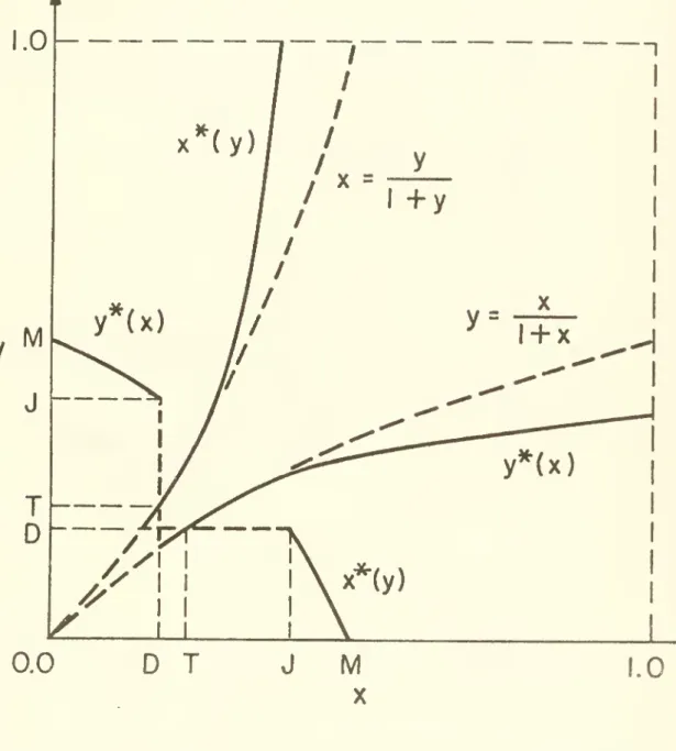
Figure 3 shows that the pair of reaction functions, x*(y) and y*(x), 12
(13)
discontinuity at D involves a drop to the A/B boundary in this case; it is never optimal to operate in Region B. For large y, x*(y) moves from the A/B boundary into the interior of Region A.
*»* INSERT FIGURE 3 NEAR HERE ***
Let us next consider Nash equilibria in this model. No such
equilibrium in x and y exists in Figure 2. In general, one can show that Nash equilibria must involve both firms operating in Region B. A
necessary condition for (x,y) to be a Nash equilibrium is thus that both
firms' first-order conditions for that Region be satisfied:
(1 - y)/9 = A/(l - x), and (1 - x)/9 = A/(l - y). (15)
These conditions are identical, however, so that in general if there is 14 one Nash equilibrium there will be a continuum of such equilibria. There exist x and y between zero and one satisfying (15) as long as A <
1/9, or M > 5/9. But this is only a necessary condition; the necessary and sufficient condition requires both firms to be in Region B, so that x
= x*(y) and y = y*(x). By the symmetry of the situation, there exist
equilibria if and only if the symmetric point x = y = 1 - t/9^ is an equilibrium. Numerical evaluation of reactions functions corresponding
to different values of M indicates that this condition is satisfied for M
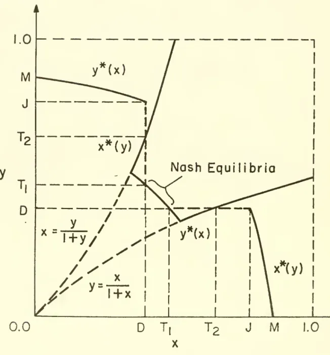
>^ E, where E is between 0.82 and 0.83. Figure 4 shows the reaction
functions for M = 0.86. All points [x*(y),y] for D < y < T^ are
Nash equilibria, as indicated. For this value of M, it is never optimal
to operate in Region A, and the discontinuity at D leads to operation in
(14)
*«« INSERT FIGURE 4 NEAR HERE ***
Finally, let us see how V varies along the reaction function. One can show that n^ is negative in Region C and positive in Regions A
and B. Thus by the envelope theorem, for any upward sloping C
schedule, V^ is reduced by increases in y for y < D, minimized at y =
D, and increased by increases in y for y > D. Further, D is always
less than M, as in Figures 3 and 4. Since reaction functions are
negatively sloped in Region C, J < M, where J is the limiting value of x»(y) as y approaches D from below. (See Figures 3 and 4.) Since the point X = J, y = D is in X's Region C, it must be that J > D/(l - D)
> D, so that M also exceeds D as asserted.
V. Advertising by the First Entrant
We are now in a position to analyze the optimal choice of x by firm
X, the first entrant, on the assumption that it knows that Y will appear
after x has been chosen (and advertising leaflets have been sent to
potential buyers) and contemplate entry. The results depend on what is
assumed about X's options after Y's entry; we consider two cases. In the first case, X can credibly commit not to increase x after Y's entry, so
that X will in fact never change. (Since buyers never forget, decreases
in X or y are not possible, just as decreases in production capacity are
usually ruled out in the corresponding literature. ) Under some
conditions, destruction of the materials necessary to print more leaflets may serve to accomplish this. In the second case, X cannot make such commitments and is restricted to credible x's, defined as those values of
X such that X will not wish to increase advertising if Y enters on its reaction function. Formally, x^ is credible if and only if
(15)
x*[y*(xo)] < xq (16)
In Figure 3, x is credible unless it is less than T. In Figure 4,
there are two ranges of credible x's: D
£
x£
T, and x >^ T^.If X selects a credible x, Y's best response if it enters is y*(x), and the game is over. If X cannot commit in advance not to increase x and it
selects an x that is not credible, the situation becomes quite complex.
Both X and Y must analyze possible sequences of increases in x and y over
time. Limiting X to credible advertising levels avoids the necessity of
solving such dynamic games, but it may over-state the effects of X's inability to commit not to increase advertising after Y's entry.
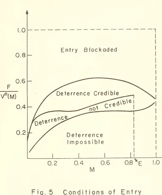
If F is large enough, entry will be blockaded in the sense of Bain
(1956) in both cases. That is, if X sets x = M, as if entry were
impossible, and V^[M,y*(M)] is less than F, Y's entry will be
deterred. (The point x = M is always credible. ) The upper boundary
in Figure 5 is derived by setting F equal to this critical value and scaling by X's present value net of leaflet preparation costs. (If F >_
v'"(M), the market is not profitable for X even if it is free from the threat of entry.
)
»** INSERT FIGURE 5 NEAR HERE »**
If entry is not blockaded, it is necessary to make some assumption
about X's post-entry options. Let us deal first with the simple case in which the x it selects is never changed. Given the threat of Y's entry,
X can either select the Stackelberg value of x, which maximizes V [x,
y*(x)] in anticipation of Y's arrival, or it can attempt to deter Y's entry. Since V^[x, y*(x)] is minimized at x = D and increases in x for
(16)
an attempt to deter entry. Such over-investment in introductory
advertising would make entry more attractive to Y, not less attractive. Entry deterrence thus must involve setting x between D and M. If F <
V^[D, y*(D)], deterrence is impossible, since the minimum value of W^
that X can impose is non-negative. The lowest curve in Figure 5 presents
a numerical evaluation of this critical level of F, scaled as before. If F is between the upper and lower critical levels, so that
deterrence is neither unnecessary nor impossible, X's optimal strategy is
found by comparing the profits yielded by optimal deterrence with those
obtained at Stackelberg equilibrium (with X as leader). One can show
that V (x) is concave, so that the most profitable deterrence strategy involves setting x as close to M as possible. This is accomplished by choosing the unique x between D and M such that F = V^[x, y*(x)]. At
this point, (6) gives X's present value. The Stackelberg return, to which this must be compared, is found by maximizing V [x, y*(x)]. In
fairly extensive computations, deterrence was always more profitable than
Stackelberg equilibrium when F was between the upper and lower critical 18
levels. It is thus apparently always optimal in this model to deter entry when deterrence is both possible and necessary and x can commit never to increase its advertising after Y's entry. But, in sharp contrast to models involving investment in production capacity, deterrence is here accomplished by under-investment relative to the monopoly level, not over-investment.
If deterrence is impossible, and apparently only then, X's best
policy is to act as a Stackelberg leader in anticipation of Y's entry.
For all values of M > 0.06 for which computations were performed, this policy called for X to select the smallest x less than D at which the
19
relevant functions were evaluated. Thus Y's post-entry profits are apparently generally minimized at X's Stackelberg point. While y is
(17)
indifferent between x's just above and just below D, X prefers the latter because they Induce sharply larger values of y from which it benefits. At least for M >^ 0.06, and possibly more generally, y exceeds x at X's
Stackelberg point, as Figures 3 and 4 suggest. In this case, X's
position as first mover enables it to capture advantages associated with being small relative to its rival; V exceeds V^ at all Stackelberg
points computed.
The results change in interesting ways when X is restricted to credible x's. In order for deterrence to be possible in this case, F
must exceed the minimum value of V^[x, y*(x)] over all credible x's.
In Figure 3, x's below T are not credible, so that if F is less than V^[T, y*(T)], it is not possible to deter entry credibly. In Figure 4,
however, points arbitrarily close to D are credible, and the credibility
constraint does not reduce the set of F's for which deterrence is
possible. The middle curve in Figure 5 is a numerical evaluation of the 20 upper bound of the region in which credible deterrence is impossible.
Note that at M = E, where Nash equilibria in x and y come into existence
and the geometry changes from that of Figure 3 to that of Figure 4, this
curve drops discontinuously to the lower curve, with which it coincides for all M > E.
If deterrence is neither impossible nor unnecessary, we must again
compare deterrence profits with those obtained by Stackelberg leadership. The Stackelberg return is found by maximizing V [x, y*(x)] over
credible values of x. In all cases for which computations were performed, V^Cx) exceeded this return for all credible x's between D
21
and M. Thus, even if X is limited to credible values of x, it is
apparently optimal to deter entry whenever possible. As before, deterrence must always involve advertising less than a protected monopolist would.
(18)
Finally, if deterrence is impossible, and, again, apparently only then, X's optimal policy is Stackelberg leadership. The credibility constraint (16) is apparently always binding: none of the unconstrained
stackelberg points computed satisfied it. In this case, V [x, y*(x)] 22
was always maximized at the smallest credible x examined. For M <
E, when no Nash equilibria exist, X thus apparently optimally chooses a
point like T in Figure 3 if Y's entry is inevitable. As that Figure suggests, y*(x) was less than x at all such points examined, and V^ exceeded V . Since x cannot be credibly set below y*(x) for M < E,
the credibility constraint apparently makes it better to enter second
than firstI For M > E, values of x arbitrarily close to E become credible, as in Figure 4, and computations indicate that X optimally
23
selects the Nash equilibrium with the smallest possible value of x.
At such points V^ exceeds V^, though y*(x) exceeds x. When Nash
equilibria exist, there is thus apparently still an advantage In entering first even though later entry cannot be deterred. As before, that
advantage turns on the ability to be small relative to the later entrant.
VI. Conclusions
The assumptions stated in Section I were chosen in an attempt to produce a simple model resembling as closely as possible models in which
over-investment in production capacity may credibly deter entry, while 24 allowing advertising to have plausible effects on buyers' behavior. The resulting model turned out to be of surprising (to me, at least)
complexity and to differ in basic ways from the models after which It was
patterned. Here, as in those models, durability and scale economies can
interact to produce blockaded entry. But if entry is not blockaded, optimal deterrence here Involves under-investment, whereas deterrence strategies involving production capacity employ over-investment.
(19)
Moreover, this model exhibits pervasive disadvantages of size that do not have analogs in most models not involving advertising.
The analysis presented here suggests that the strategic implications of investments in at least some kinds of advertising may differ
dramatically from those of investments in tangible, productive assets. Two sources of such differences come to mind. First, investment in
productive assets affects the relation between cost and units of output, while investment in advertising fundamentally acts on Individuals' demand
curves. When individual buyers can vary the number of units they purchase, as in this model, this formal difference may have basic strategic implications. Second, investment in productive capacity
generally discourages entry by making lower prices more attractive to the incumbent. But investment in advertising that provides the Incumbent
with a set of loyal customers that would not find an entrant's wares
attractive (perhaps, as here, because they would be unaware of the
entrant's existence) may make it less eager to cut price in response to entry and give up profits that could be earned from those loyal
customers. With price discrimination ruled out, as it is here, an incumbent's investment in advertising may make entry more attractive by
25
guaranteeing the entrant a friendlier welcome. Both these factors are present in this model. The second is clearly visible in the
post-advertising equilibria of Section III, and it appears to drive the main results obtained here.
I do not claim that the model presented in this essay provides a
useful description of most markets or indeed of any actual market. While
I think its assumptions are natural and have some plausibility, its results run counter to the intuitions of many economists and to some
26
(20)
see exactly what features of this model drive those results and to delineate the conditions under which over-advertising can optimally and credibly deter entry.
(21)
References
Bain, J.S. Barriers to New Competition. Cambridge, Mass.: Harvard University Press, 1956.
Baldanl, J., and Masson, R.T. "Economies of Scale, Strategic Advertising and Fully Credible Entry Deterrence." Cornell University, Mimeographed December 1981.
Baumol, W.J., and Willig, R.D. "Fixed Costs, Sunk Costs, Entry Barriers, and Sustainability of Monopoly. " Quarterly Journal of Economics 96
(August 1981): 405-31.
Butters, G.R. "Equilibrium Distributions of Prices and Advertising." Review of Economic Studies 4A (October 1977): 465-92.
Comanor, W.S., and Wilson, T.A. "Advertising and Competition: A Survey." Journal of Economic Literature 17 (June 1979): 453-76.
Dixit, A.K. "The Role of Investment in Entry Deterrence." Economic Journal
90 (March 1980) : 95-106.
. "Recent Developments in Oligopoly Theory." American Economic Review 72 (May 1982): forthcoming.
Eaton, B.C., and Lipsey, R.C. "Capital, Commitment and Entry Equilibrium." Bell Journal of Economics 12 (Autumn 1981): 593-604.
Gelman, J.R., and Salop, S.L. "Judo Economics, Entrant Advantages, and the Great Airline Coupon Wars." Mimeographed, Georgetown University, March 1982.
Scherer, F.M. Industrial Market Structure and Economic Performance, 2nd
Ed. Chicago: Rand-McNally, 1980.
Schmalensee, R. "Economies of Scale and Barriers to Entry." Journal of
Political Economy 89 (December 1981): 1228-38.
. "Product Differentiation Advantages of Pioneering Brands." American Economic Review 72 (June 1982): forthcoming.
(22)
Spence, A.M. "Entry, Capacity, Investment and Oligopolistic Pricing." Bell Journal of Economics 8 (Autumn 1977): 534-44.
. "Notes on Advertising, Economies of Scale, and Entry
(23)
Footnotes
I am Indebted to the National Science Foundation for financial support, to Severin Borensteln for excellent research assistance, and to
participants In a seminar at the University of Toronto for valuable
comments on an earlier version of this essay. The usual waiver of liability applies.
1. See, for Instance, Scherer (1980, pp. 246-8).
2. Dixit (1982) has recently provided a clear summary of this work. He
also discusses complementary work on "reputation effects," which are ignored here.
3. The seminal paper here is Spence (1977), which focuses on durable Investment but does not deal with credibility. The result stated in the text seems due to Dixit (1980); see also Schmalensee (1981) and Dixit (1982). The importance of investment durability is made clear by Eaton and Llpsey (1981).
4 There is a good deal of controversy about both durability and scale economies; see Comanor and Wilson (1979).
5. Spence (1977, 1980) has dealt with advertising in this context, but his models suffer from the same basic problem as the Bain/Sylos
analysis.
6. Baumol and Willig (1981) have recently stressed the conceptual importance of the distinction between fixed and sunk costs.
7. One can show that a necessary and sufficient condition for a monopoly secure against entry to have a positive w"" is that c(x)/x attain
its minimum at x < M.
8. Suppose the contrary, and assume that equilibrium involves q's such that p^ > p . Then X must sell only to the x(l - y) buyers who
(24)
know only of it, and Y sells to all y who are aware of It. It is
then clearly optimal for X to obtain the monopoly price, p*, from its captive audience by producing the corresponsing monopoly quantity,
x(l - y)(l - c)/2. But Y can raise its price (by lowering its output) and increase its profits until it too obtains the monopoly
price from its customers.
9. This is intimately related to the "judo economics" of Gelman and Salop (1982). They find that a potential entrant that can credibly
limit its output may be able to profitably enter against an established monopoly despite demand and cost disadvantages.
10. Subscripts are used to denote partial derivatives here and in all that follows.
11. Use of the limiting values of n^ shown in Figure 2 establishes
that sufficient conditions for x* not to lie in B or C are (a) A/[l
-y/(l + y] > (1 - y)/9, and (b) either y > 1/2 or A/[l - y/(l
-y)]
17(1
- y)/27. The first of these is satisfied for y > (1-9A)/(1 + 9A), and the second is satisfied for y > (7 - 27A)/14. Both of these critical values are always less than one. So if y is
close enough to unity, x»(y) must be either in Region A or on the A/B boundary.
12. The profit function in (13) is such that points on the reaction
function cannot generally be obtained analytically. Proceeding as in
footnote 11, the program employed first ascertains the Regions in which solutions to (14) exist, and it checks to see if x* may be on
the A/B boundary. It then computes solutions to (14). In Regions A
and C, this requires numerical evaluation of the relevant roots of fourth degree polynomials. A direct comparison of profits is used to determine x* if multiple candidate values are thus identified.
(25)
13. There can be no equilibria with either firm on the A/8 boundary, since this would imply that the other was on the B/C boundary, and it
is never optimal to operate there. Suppose an equilibrium exists with X in Region A and y in Region C. Then if z = x/(l - x),
equilibrium involves z < y. Writing down the corresponding
2
first-order conditions and solving both for A(l + z)(2y + z) /y,
one finds that an equilibrium of this sort.
T(z;y) = z^ +
z^Cyd
- y)] + z[3y2(l - y) - 3y]+ 2y^[y(l - y) - 1] = 0.
To show that no equilibria outside Region B exist, it suffices to
show that this equation, treated as a cubic in z for given y, has no
real roots between zero and y. Since the maximum value of T(y,y) is negative, T is always negative when z = y. Since T must be positive for large z, T(z;y) = thus has one real root larger than y. At z =
0, T is negative and decreasing in z, it attains a local maximum at some negative z, and it is clearly negative for large negative values
of z. It thus follows that T(z;y) = has either a pair of negative
roots or a pair of complex roots. Since it has no real roots between zero and y, the proof is complete.
14. This is a property of the particular C(x) function assumed here. If
C(x) = F + Ax/(1 - x), which has roughly the same shape, there is at most one Nash equilibrium for any value of A. For this cost
function, numerical evaluation of the reaction function indicates
that such equilibria exist for all A
£0.035,
which corresponds toM > 0.626.
(26)
16. By the shapes of reaction functions in this model, if x*(l) <_fA, it follows that X = M is credible, since X will never want to raise x no
matter what Y does. Footnote 11 establishes that x»(l) is either in
Region A, with x* < y/(l + y) = 1/2, or on the A/B boundary with X* = 1/2. Referring to Figure 2, x* is on the boundary if and only if (5 - y)/27 > A/[l - y/(l + y)], or A < 2/27. But A < 2A27
implies M = 1 - 4A > 19/27 > 1/2. Thus x*(l) < M for A <
2/27. For all larger A, X's Region A first-order condition when y =
1 is
(2 + 3z - 2^)/(2 +
zP
= A(l + z),where
£
z = x/(l - x) _< 1. At z = 0, the left-hand side ofthis equation equals 1/4, while the right-hand side equals A, which
is less than 1/4. The left-hand side is decreasing in z, so that A(l
+ z) < 1/4 at a solution. Substituting for z, this last inequality
establishes that x*(l) < M for A > 2.27 as well, and the proof is
complete. (In Figure 3, A > 2/27, while A < 2/27 in Figure 4.)
17. For M = 0.02, 0.04, ..., 0.98, we searched over x = 0.002, 0.004,
..., 0.998 to find the minimum value of V^Ex, y»(x)]. Since the true minimum was thus never found exactly, the lowest curve in Figure
5 is too high by an unknown but probably small amount. For small M
the search over x involves a coarse grid in the relevant region, and
the results are correspondingly less reliable. (Indeed, some model properties known to hold globally were violated in the output for M =
0.02 and M = 0.04.) While some of the general results suggested by
these computations and described in what follows may be susceptable
to analytical proof, this model is both so special and so
(27)
conclusions hardly seems worth the substantial effort that would be required.
18. See footnote 17. The Stackelberg profit was taken to be the largest
value of V^[x, y*(x)] encountered, and this was compared to s/^(x)
Tot all x's examined between D and M.
19. See footnote 17. Results for M = 0.02 and 0.04 are suspect for the reasons noted there. The finding reported in the text suggests that
X's Stackelberg point is strictly undefined, as there is no "largest
x less than D".
20. The procedure described in footnote 17 was used, except that the search was restricted to values of x passing the credibility test, given by inequality (16) in the text.
21. See footnote 17.
22. See footnote 19.
23. Again, this means that X's Stackelberg point may be undefined, as there is in general no "Nash equilibrium with the smallest x".
24. Baldani and Masson (1981) allow the incumbent monopolist to invest in "goodwill," which determines post-entry share but does not affect pre-entry sales. It is not clear what assumptions about buyer
behavior would produce such a demand structure, though aggregate
structures involving "goodwill" are commonly assumed.
25. See footnote 9.
26. In particular, these results seem at odds with recent theoretical and empirical work that points to general advantages enjoyed by
pioneering brands; see Schmalensee (1982) and the references there
cited. This comparison suggests the importance of the assumption here that advertising removes all uncertainty about product quality.
0.25
0.20
-0.15
0.10
0.05—
Fig.
1n^
(x,y)/x
0.25
0.20-0.15
0.10-
0.05-C^(x)
y
=0.25l
Fig.
2
n