FDI convergence and Spatial Dependence between Chinese Provinces

HAL Id: halshs-00570498

https://halshs.archives-ouvertes.fr/halshs-00570498

Preprint submitted on 28 Feb 2011

HAL is a multi-disciplinary open access archive for the deposit and dissemination of sci-entific research documents, whether they are pub-lished or not. The documents may come from teaching and research institutions in France or abroad, or from public or private research centers.

L’archive ouverte pluridisciplinaire HAL, est destinée au dépôt et à la diffusion de documents scientifiques de niveau recherche, publiés ou non, émanant des établissements d’enseignement et de recherche français ou étrangers, des laboratoires publics ou privés.

FDI convergence and Spatial Dependence between

Chinese Provinces

Nasser Ary Tanimoune, Mary-Françoise Renard

To cite this version:

Nasser Ary Tanimoune, Mary-Françoise Renard. FDI convergence and Spatial Dependence between Chinese Provinces. 2011. �halshs-00570498�

5th _{INTERNATIONAL CONFERENCEONTHE CHINESE ECONOMY}

China in the World Economy: Internal Challenge and International Challenges IDREC-CERDI, Université d’Auvergne

FDI convergence and Spatial Dependence between Chinese

Provinces

Nasser Ari Tanimoune, CERDI, University of Auvergne Mary-Françoise Renard, IDREC-CERDI, University of Auvergne

Abstract : This study aims at investigating the spatial dimension of the FDI. Considering the distribution of FDI between the provinces, our purpose is the spatial dependency that may be observed. Using data for 1992-2002, we find that taking into account the regional specification induces significant FDI convergence process between Chinese provinces. We also find that correcting for the bias resulting from spatial autocorrelation in errors terms leads to higher estimates of the beta convergence coefficients. One can deduce that this is somewhat important for Chinese authorities to promote an attractivity policy based on regional complementarities rather than on FDI quantity

JEL Classification :

Keywords : FDI, China, Spatial autocorrelation, Provinces

1.Introduction

The Open-door policy reflected the objectives of the Chinese authorities to encourage the openness of the Chinese economy. It has been adopted by the Central Committee of CCP in 1978. Trade and besides Foreign Direct Investment (FDI) have been concerned. It was a dramatic change in Chinese policy, which generated large flows of FDI, sustaining a high growth rate, especially of exports.

This new FDI policy may be divided in three stages (Zhang, 1999, Sun et alii, 2002). The first stage began in 1979 when the “law of People’s Republic of China on Joint Ventures using Chinese and Foreign Investment” was enacted. At the beginning, investments grew slowly in spite of the creation of Special Economic Zones. This slow growth was the result of a lack of infrastructures and of juridical institutions. In 1983, the State Council decided to increase the liberalisation and created 14 “coastal cities”. So, the FDI expanded but a slow down may be observed in 1985 explained by the inflation and by a legal environment poorly defined.

A second stage begins in 1986 with a new law promulgated in April: the Law on Enterprises Operated Exclusively with Foreign Capital. This law and different amendments, relaxed the constraints on foreign investment and enhance property rights. In October, a new decision lightened the administrative constraints and enlarged tax exemptions. Moreover, local governments have got a growing power concerning the FDI. In 1987, the first guide for investment defined which sector is a priority and which is forbidden for foreign investors. The prohibited measures look like incentives for investments from foreign firms which don’t have to take care of the Plan and which benefit from a lot of privileges; for instance, they pay the same price as State-own enterprises for electricity or transportation, and they can exchange currencies. At the end of 1989, with Tienanmen Square events, the FDI flows declined.

A third phase began around 1990, with a regular and strong increase of FDI. To compensate the western criticisms against China, the government proposed some new tax facilities and Deng Xiaoping went for a trip in the south of the country to promote China next to foreign firms. FDI’s growth has been 150% in 1991 et foreign firms became numerous since this year.

One of a main characteristic of this phenomenon is the geographical dimension. At the beginning, the creation of the Special Economic Zones, the only places allowed to receive FDI, intended to attract investment from Honk Kong, Taïwan and Macao. This strategy was very unequal from a spatial point of view and FDI location generated great disparities; the regional gap widend in 1992 (Bao et alii). But the objective was to generate spillover effects and to distribute the coastal provinces growth between the other regions.

Most of the studies about convergence have a temporal dimension. The topic of this paper is to focus on the spatial dimension.

It studies the existence of spatial dependency in the dynamic of FDI. The implications are important as the disparities are growing between Chinese provinces and as the regional policy plays a significant role. The Chinese government tries to promote investments in western provinces and some studies underlined the difficulties for these provinces to attract FDI or to benefit from FDI located in the other provinces (Brun et alii, 2002, Wen, 2004).

Now, if a spatial dependency exists between provinces, the best policy does not consist to attract FDI. It is more efficient to set up an industrial policy to develop complementarities accross provincial industries. This is a quite different strategy and which means that the government has to choose between a catching up policy or a complementary policy.

In its generic form, the term of convergence suggests that there exists a way by which impover-ished countries can catch up richer ones in terms of level of income. Initially, the convergence process is empirically investigated through growth regressions. The catching up of wealthy coun-tries by poor ones takes place if there exists a negative correlation between growth and initial in-come. Applied to FDI levels in China, the convergence analysis deals with the manner to define a policy framework to attract FDI as they become a key explanatory variable of the spectacular growth observed in China.

To the contrary of previous specifications in the literature1_{, we apply a spatial panel data model to}

analyze regional convergence of FDI process in China2. There is a growing literature which

considers the spatial localization as a key variable for understanding some aspects of China’s economy. Some recent researches began to follow this path by studying proximity effects (Amiti, 2005), neighbourhood effects (Luo, 2005), and overall those using spatial econometrics (Aroca et alii, 2005). We are then really in a spatial dimension of the Chinese growth.

But to the best of our knowledge, this is the first empirical research which accounts for spatial fixed effect panel data models in the context of FDI convergence in China. For the empirical study, we use data for the 29 provinces, excluding Tibet.

1 _{The spillovers are in general the main way for considering spatial externalities among regions. Empirically, the}

standard method consists to impose a dummy variable. For example, in China’s case of growth study, Demurger and al. (2002) impose a dummy for coastal regions.

2 _{It’s noteworthy to underline that the spatial dependence analysis become important in empirically investigating}

regional growth convergence since it seems to be introduced by Rey and Montouri (2000). Following spatial specification models developed Anselin (1988), most of the studies used cross-sectional regressions. For example, more recently the result reported by Hewings et al. (2005) analyzing the convergence among 163 regions of European Union, is that taking into account the spatial dependence can lead to new implications. They found that speeds of convergence were different depending of the regions that compose the two regimes previously identified. Elhorst (2003) develops spatial dependence panel data models which are the extension of spatial cross-sectional models. Relating to this framework, Arbia and Piras (2004) analyzed the regional convergence among European regions and found that estimations that leave out spatial effects conduce to biased results.

I : FDI dispersion between provinces

Relating to the FDI evolution in China, 1992 seems to correspond to the beginning of the

important economic growth of FDI that characterized the country3_.

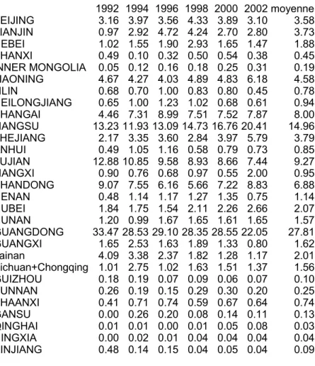
Table 1: Proportion of FDI by province (billions Yuan constant 1992 prices)

1992 1994 1996 1998 2000 2002 moyenne BEIJING 3.16 3.97 3.56 4.33 3.89 3.10 3.58 TIANJIN 0.97 2.92 4.72 4.24 2.70 2.80 3.73 HEBEI 1.02 1.55 1.90 2.93 1.65 1.47 1.88 SHANXI 0.49 0.10 0.32 0.50 0.54 0.38 0.45 INNER MONGOLIA 0.05 0.12 0.16 0.18 0.25 0.31 0.19 LIAONING 4.67 4.27 4.03 4.89 4.83 6.18 4.58 JILIN 0.68 0.70 1.00 0.83 0.80 0.45 0.78 HEILONGJIANG 0.65 1.00 1.23 1.02 0.68 0.61 0.94 SHANGAI 4.46 7.31 8.99 7.51 7.52 7.87 8.00 JIANGSU 13.23 11.93 13.09 14.73 16.76 20.41 14.96 ZHEJIANG 2.17 3.35 3.60 2.84 3.97 5.79 3.79 ANHUI 0.49 1.05 1.16 0.58 0.79 0.73 0.85 FUJIAN 12.88 10.85 9.58 8.93 8.66 7.44 9.27 JIANGXI 0.90 0.76 0.68 0.97 0.55 2.00 0.95 SHANDONG 9.07 7.55 6.16 5.66 7.22 8.83 6.88 HENAN 0.48 1.14 1.17 1.27 1.35 0.75 1.14 HUBEI 1.84 1.75 1.54 2.11 2.26 2.66 2.07 HUNAN 1.20 0.99 1.67 1.65 1.61 1.65 1.57 GUANGDONG 33.47 28.53 29.10 28.35 28.55 22.05 27.81 GUANGXI 1.65 2.53 1.63 1.89 1.33 0.80 1.62 hainan 4.09 3.38 2.37 1.82 1.28 1.17 2.01 Sichuan+Chongqing 1.01 2.75 1.02 1.63 1.51 1.37 1.56 GUIZHOU 0.18 0.19 0.07 0.09 0.06 0.07 0.10 YUNNAN 0.26 0.19 0.15 0.29 0.30 0.20 0.25 SHAANXI 0.41 0.71 0.74 0.59 0.67 0.64 0.74 GANSU 0.00 0.26 0.20 0.08 0.14 0.11 0.13 QINGHAI 0.01 0.01 0.00 0.01 0.05 0.08 0.03 NINGXIA 0.00 0.02 0.01 0.04 0.04 0.04 0.04 XINJIANG 0.48 0.14 0.15 0.04 0.05 0.04 0.09

Table 1 gives the values of the logarithm of FDI inflows into Chinese provinces during

1992-2002 period, in billions of Yuan at constant 1992 prices4_{. At this time, Chinese authorities had}

implemented important measures to attract foreign investments by reducing several restrictions. One of the core features of attractivity policies in China is the goal to attract the largest amount of FDI among al the provinces, in particular comparatively to the costal region.

3 _{For an extensive details of FDI evolution, cf. Ho (2004).}

I.1 :The dispersion over the time

The FDI dispersion overtime can be appreciated from the analysis of the sigma convergence5.

Sigma convergence occurs if the dispersion in FDI declines. In the way to catch such kind of convergence process between Chinese provinces, we used two indicators: the measure of the dispersion around the total FDI average (the traditional standard deviation indicator) and the dispersion around each provincial FDI average, called respectively conventional sigma-convergence (CSC) and referential sigma-sigma-convergence (RSC). While the first indicator informs on the dispersion between all the provinces over the time, the referential sigma-convergence reports on the FDI harmonization relatively to specific regions.

Let denotes LFDIt,i, the logarithm of the foreign direct investments in Yuan constant 1992 prices

at time t _{in the province} i; MLFDIt, the simple average of the FDI for all the i provinces at time

t _and MLFDIRk,t the simple average of the FDI of the region k at time t, with

}

{

CostalRegion,CentalRegion,Western Region

=

k 6.

The conventional sigma-convergence (σ

[

LFDIt

]

) is measured as follows:

[

]

_∑

(

)

= − = N i t i t t N MLFDI LFDI LFDI 1 2 , σ

with N the total of provinces. The referential sigma-convergence (σ

[

LFDIRt,k

]

), calculated for each

k region, is given as:

[

]

_∑

(

)

= − = N i k t i t k t N MLFDIR LFDI LFDIR 1 2 , , , σ

As it appears in the graph 1a, the slight convergence observed for 1996-2002 only reduced the di-vergence occurred over the period 1993-1996. Over the whole period, there does not seem to be any evidence of conventional sigma convergence, that is to say the FDI dispersion between all provinces did not significantly decrease.

5 _{Cf. Barro and Sala-i-Martin (1995) for details.} 6 _{For the regions’ components, see appendix.}

Figure 1a: Conventional Sigma-convergence of the natural logarithm of FDI (Yuan 92)

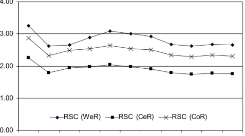
Figure 1b: Referential Sigma-convergence of the natural logarithm of FDI (Yuan 92)

Although the trend of the different referential sigma-convergence (RSC) compared to the evolu-tion of the convenevolu-tional sigma-convergence is quite identical, the dispersion are greater when the Costal and the Western Regions (respectively CoR and WeR) are taken as a reference.

It appears that harmonization of FDI over the time is not revealed. Meanwhile, the dispersion is significantly different when we refer to the regional localization of the FDI.

Al least, this observation suggests the importance of the geographical dispersion in the analysis of the FDI in China.

LFDI Sigma-convergence (Standard Error) 0.00 1.00 2.00 3.00 1992 1993 1994 1995 1996 1997 1998 1999 2000 2001 2002

LFDI Referencial sigma-convergence

0.00 1.00 2.00 3.00 4.00 1992 1993 1994 1995 1996 1997 1998 1999 2000 2001 2002

RSE(WeR) RSE(CeR) RSE(CoR)

I.2 :The spatial dispersion of FDI

To assess the importance of spatial dispersion of FDI in China, we used the Exploratory Spatial Data Analysis. For this purpose, we explored the geographical localisation of FDI between Chinese provinces. Then, in the aim to test if the potential spatial dependence effect is significant, we performed Moran’s I test of spatial autocorrelation.

I.2.1 : The provincial distribution

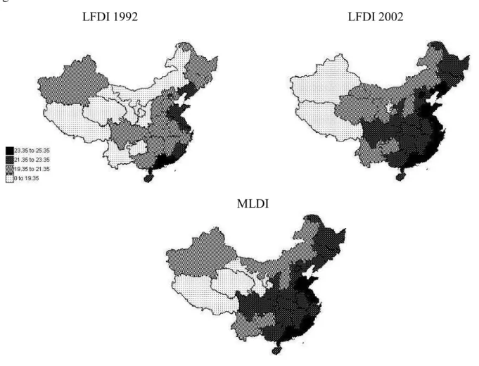
Figures below present the geographical localization of FDI inflows in Chinese provinces for the years 1992, 2002 and on average on the whole period (1992-2002).

Figure 2: Provincial distribution of FDI in China

As it appears from figure 1a and 1b, the 2002’s distribution of FDI among provinces is sensibly different than the 1992’s original distribution. Nevertheless, in all cases the two maps indicate

LFDI 1992 LFDI 2002

that there exists a strong presumption of spatial autocorrelation in the sense that at least two provinces attracting the largest (respectively the smallest) amount of FDI are contiguous.

We explored this potential spatial autocorrelation by testing for regional similarity using Moran’s I test statistic.

I.2.2 : The spatial autocorrelation of FDI localization

As noted by Anselin (1988), the starting point of an analysis of spatial dependence is to define exogenously the geographical arrangements that drive the data observations called the spatial

weight matrix (W). It’s composed by wi,j, the

( )

i,j th element

(

i, j=1,...,N

)

of a N*N matrix.

For the analysis of the FDI spatial localization, as spatial weight matrix, we calculated the

1st-order queen neighbors based on the longitude and latitude of all of the Chinese provinces7. Then,

considering this spatial arrangement we computed the local Moran’s I statistic (M’s I).

M’s I proposed by Anselin (1995) is a decomposition of the Moran’s I statistic (Moran 1950) into contribution for each spatial unit and allows to detect local spatial autocorrelation, that is to say to identify provinces where adjacent areas have similar FDI distribution. The test is conducted in one time period for a single variable through its z-score standardized dataset following the formula below:

∑

= j t j j i t i W m m I s M' ˆ _{, ,} ˆ _,

where mˆi,t and mˆj,t are the z-score standardized of FDI for province i and province j at time t and

j i

W_{, the spatial arrangement between the related. Under the null hypothesis, the FDI localization}

in different provinces are considered to be spatially independent. As variables are standardized, the M’s I value range from -1 to 1: a positive value means that nearby provinces have received similar inflows of FDI while a negative value indicates that contiguous provinces are characterized by dissimilar FDI.

The results of the Moran’s I statistic value and the related p-value are reported in table 2 below. Under the null hypothesis of no spatial autocorrelation, the Local Moran’s I are statistically sig-nificant at 99%. Also, the calculated Moran’s I statistic are positive.

7 _{Queen Contiguity based spatial weight matrix is created when spatial data observations are specified as polygon and}

includes boundaries and vertices allowing for more neighbors. We use STIS software to conduct the Moran’s I test and it’s related calculus.

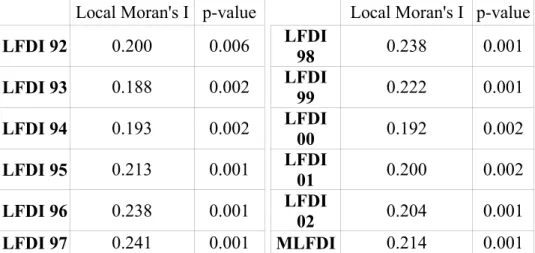
Table 2: Local Moran’s I statistic on logarithm of FDI between Chinese provinces

Local Moran's I p-value Local Moran's I p-value

LFDI 92 0.200 0.006 LFDI 98 0.238 0.001 LFDI 93 0.188 0.002 LFDI 99 0.222 0.001 LFDI 94 0.193 0.002 LFDI₀₀ 0.192 0.002 LFDI 95 0.213 0.001 LFDI₀₁ 0.200 0.002 LFDI 96 0.238 0.001 LFDI 02 0.204 0.001 LFDI 97 0.241 0.001 MLFDI 0.214 0.001

The p-value of Moran's I is calculated by using 999 Monte Carlo randomizations of the FDI dataset after us-ing the Simes adjustment correctus-ing for multiple testus-ing.

One can deduct that there exist a positive spatial dependence provincial FDI in China, over each year, from 1992 to 2002 and on average over the period. This is why a beta-convergence analysis corrected for spatial dependence bias is somewhat required for a more comprehensive analysis of FDI convergence between Chinese provinces.

II : Modelling spatial FDI convergence

II.1 : Spatial dependence panel data models

Our empirical framework is derived from growth convergence analysis (Barro and Sala-I-Martin, 1995). To analyse the evolution of FDI across China’s provinces, we use a standard FDI beta-convergence equation which functional form is as follow:

(

i

)

ti it i i i t X FDI FDI FDI ε β α + +Β⋅ + =         , , 0 , 0 , ln ln _{eq. 1}

with N provinces (i=1,...,N the 29 provinces named spatial units), T time periods (1992-2002)

and εit the disturbance assumed to be normally distributed with zero mean (E(εit)=0) and to

have constant variance (E(εit2)=σ2IN). As the left-term is the growth rate of the real FDI on the

entire period, the FDI0,i term is the real FDI of the province i at the beginning of each period and

i t

The estimation framework is as follow (Anselin and Bera, 1998),. In a first step, we estimate an Ordinary Least Square fixed effect model (FEOLS) that is to say without spatial consideration. Then, we check for the presence of spatial autocorrelation given the Lagrange Multiplier test based on the Ordinary Least-Square residuals (LMSEM) as proposed by Anselin (1988):

) 1 ( ˆ ˆ * ). ( 1 2 2 2 χ σ ε ε →       ′ ⋅ ′ + = W W W W tr LMsem eq. 2

where εˆ is the FEOLS residuals, W the spatial weight matrix and σ² the variance term. In case

of rejection of the null hypothesis of no spatial dependence, we estimate a fixed effect spatial error model (FESEM) in order to correct the spatial dependence nuisance in the residuals. The (N,T) panel data equation to estimate as proposed by Elhorst (2003) is:

(

i

)

ti it i i i t X FDI FDI FDI ε β α + +Β⋅ + =         , , 0 , 0 , ln ln _with ε_it =λWε_it +ϕ_it eq. 3

The FESEM equation is estimated by maximum likelihood method. In presence of spatial autocorrelation and if the estimated spatial coefficient is statistically positive (negative), we can conclude that there exist a positive (negative) spatial dependence.

We also calculated the speed of convergence (noted b) and the time necessary for the real FDI to

fill half of the variation given their steady state (τ ). These two indicators are calculated through

the following expressions:

T T b=−ln(1+ β) and τ _ln(ln(₁ 2)_β) + − =

Lastly, to assess the importance of FDI location given the three principal regions, we estimated

the beta-convergence equations related to the simple average of the real FDI of the region k for

the first period (MFDIR0,k). Hence, the equations 1, 3 and 4 are rewritten respectively as:

(

k

)

ti it i k i t X MFDI MFDI FDI ε β α + +Β⋅ + =         , , 0 , 0 , ln ln _{eq. 1’}

(

k

)

ti it i k i t X MFDI MFDI FDI ε β α + +Β⋅ + =         , , 0 , 0 , ln ln _with ε_it =λWε_it +ϕ_it eq. 3’

with CoR the Costal Region, CeR the Central Region and WeR the Western region.

If the estimated coefficient β in eqs. 1 or 3 is negative and statistically significant, we can

conclude that there is a conditional convergence of FDI in China. More specifically, in the case of eqs. 1’ and 3’, it’s mean that a conditional convergence of FDI in China regarding a given region

II.2 :Data

In the regression analysis, the spatial arrangement that characterizes China’s provinces is defined by the simple bilateral distances (SBD). The SBD are calculated from the inter-city distances between the biggest cities in the two provinces and are presented as a N*N spatial weight matrix,

W, with wi,j its

( )

i,j th element

(

i,j=1,...,N

)

. Such kind of matrix of contiguity was preferred

because it rather takes account of the distances between supposed the decision-making centers

(the biggest cities) than the length of the borders between the provinces8.

A number of factors have been mentioned and analysed as potential determinants of FDI in China (Wei et alii, 1999, Cheng and Kwan, 2000, Sun et alii, 2002).

LFDI is the explained variable measured by the logarithm of the ratio between FDI of province i at time t and the FDI of the same province at the initial date (1992). It supposed to capture the evolution of FDI. To take into account the specific evolution of FDI in each region, we use also explained variables LFDIA, LFDIB and LFDIC calculated as above, respectively the Costal, Western and Central regions.

LFDIT0 represents the initial level of the logarithm of FDI (constant 1992 prices) for each province. In a similar way, LFDITA, LFDITB and LFDITC are respectively the average of the initial level of the logarithm of FDI (constant 1992 prices) of provinces which compose the Costal, the Western and the Central region. The beta-convergence is associated with these variables.

The others variables included in the basic regressions are related to the main determinants of FDI in China (Wei et al., 1999; Cheng and Kwan, 2000; Sun et al., 2002). Among the other explanat-ory variables, LRGPC indicates the size of province’s economy, as measured by the logarithm of its gross domestic product (in constant 1992 prices). Its effect is supposed to be positive in the sense that a large economy is associated with more FDI inflows in relation with the potential mar-ket activities. The marmar-ket demand and marmar-ket size have positive impact on the FDI because it af-fects the expected revenue of the investment (Sun and alii, 2002).

LEXIM is an indicator of the province’s trade balance. It is measured as the ratio of exports to imports. The related coefficient is supposed to be negative when imports increase (or when exports decrease), the ratio should slow the growth of the FDI (see Sun et alii, 2002).

LVFR is supposed to highlight the importance of transportation infrastructures in determining FDI location in each province. The indicator used is the logarithm of the sum of the rail ways and

of roads9. A positive effect is expected as more transportation infrastructures lead to greater FDI

evolution.

8 _{Another technical motivation is that the original program for estimating a spatial panel fixed effect model is written}

in Matlab codes by Elhorst. The programs is provided by the author on is web site (**). However, we adapted the Lagrange multiplier tests from Elhorst’s programs and Lesage’s Matlab Spatial estimation Toolbox. The econometrics estimations are conducted with Matlab software. All the programs used are available upon request.

9 _{Note that, as others studies in this field, we make the implicit assumption that these different transportation modes}

LRAW is an indicator for labour cost. This variable should have a negative impact on the FDI evolution as province with lower wage rate can expect to be more attractive for FDI. It is measured as the logarithm of the ratio of wage to provincial GDP (constant 1992 prices).(see for instance Coughlin and Segev, 2000).

III : Results

First at all, the results show that the β-convergence models without correction by spatial dependence effects (FE-OLS) appear to be fallacious. The Lagrange Multiplier test on the Ordinary Least-Square residuals (LMsem) leads to reject the null hypothesis of no spatial correlation at 95% level of confidence. In other words, the FE-OLS estimation exhibits significant spatial correlation in the residuals. Also, the estimated coefficient of the spatially

correlated errors (λ) in the fixed effect spatial error model estimation appears significantly with

99% level of confidence.

Given the global results of all the regressions, it appears that a spatial dependence models with spatially autocorrelated errors can be seen as lightly more appropriate to make inference.

FE-OLS FE-SEM

LFDI LFDIA LFDIB LFDIC LFDI LFDIA LFDIB LFDIC

LFDIT0 _(1.00)0.14 _(1.00)0.15 LFDITA -0.30_(0.10) -0.25*_(0.01) LFDITB -0.49*_(0.00) -0.52*_(0.00) LFDITC -0.35***_(0.05) -0.32*_(0.01) LRGPC 1.67*_(0.00) 0.93*_(0.00) 1.40*_(0.00) 0.88*_(0.01) 1.62*_(0.00) 0.62**_(0.02) 1.61*_(0.00) 0.70**_(0.03) LEXIM -0.21**_(0.03) -0.30*_(0.00) -0.30*_(0.00) -0.32*_(0.00) -0.23*_(0.01) -0.16**_(0.04) -0.27*_(0.00) -0.27*_(0.00) LVFR _(0.33)0.12 _(0.16)0.17 _(0.22)0.14 _(0.19)0.16 _(0.31)0.12 0.19***_(0.08) 0.19***_{(0.08) (0.22)}0.14 LRAW -0.78*_(0.00) -0.60*_(0.01) -0.72*_(0.00) -0.56*_(0.01) -0.73*_(0.00) -0.45**_(0.02) -0.94*_(0.00) -0.47**_(0.03) Lambda _(0.44)0.14 0.99*_(0.00) 0.99*_(0.00) 0.54***_(0.05) R² 86.4 95.8 95.8 95.7 86.4 96.0 96.0 95.8 Lmsem 48.48*_(0.00) 42.02*_(0.00) 39.46*_(0.00) 14.10*_(0.00)

In bracket are the P-value. * (respectively **, ***) : significant at 99% (resp. 95 and 90%), otherwise not significant.

One can also deduct that there is no FDI convergence when one considers their evolution in all the provinces even if the estimation is corrected by the spatial dependence effect. Instead, a FDI convergence takes place when the comparison is done according to the regional FDI level. In particular, the speed of FDI convergence is more important when we take as reference the average of FDI of the Western region (mainly stripped) compared to the Central region and especially the Costal region the most endowed in term of FDI. For the other variables, the estimated coefficients have essentially the awaited signs.

IV Conclusion

The aim of this paper is to investigate the FDI convergence process between Chinese provinces after correcting by spatial autocorrelation effects. We start by analysing the spatial evolution of FDI and we estimate several equations with fixed effects spatial error models.

We show that there is a significant FDI convergence process between Chinese provinces when we take into account the spatial localisation of the FDI. Also, after correcting for the spatial errors bias, the speed of convergence between provinces which attracted less FDI becomes more import-ant.

At least, this study provides evidences of the decisive aspects of time and space in the analysis of FDI in China.

References

Amiti M. et Javorcki B.S., 2005, Trade costs and location of Foreign Firms in China, IMF

Working Paper, mars.

Anselin L., 1988, Spatial Econometrics: Methods and Models, Dordrech, The Netherland: Kluwer Academic Publisher.

Anselin L. and A.K.Bera, 1998, Spatial Dependence in Linear Regression Models with an Introduction to Spatial Econometrics, in Ullah and Giles (Eds) Handbook of Applied Economic

Statistics, M.Ockker, NY, Chap.7.

Arbia, G., 2004, “Alternative approaches to regional convergence exploiting both spatial and temporal information", Paper presented at the first seminar Jean Paelinck, University of Zaragoza, Zaragoza, Spain, October 2004.

Aroca P., Guo D. et Hewings G.G.D., 2005, Spatial convergence in China: 1952-1999”, presented at the Conference “Inequality and Poverty in China”, UNU-WIDER, Helsinki, août.

Bao S., Chang G.H., Sachs J., WO W.T., 2002, Geographic factors and China’s regional development under market reforms, 1978-1998, China Economic Review, 13, 89-111.

Barro R.J., Sala-i-Martin, 1995, Economic Growth, New-York, McGraw-Hill, Inc.

Brun F.F., Combes J.L., Renard M.F., 2002, Are there spillover effects between coastal and non coastal regions in China, China Economic Review, 109, 1-9.

Cheng L.K. and Kwan Y.K., 2000, What are the determinants of the location of foreign direct investment? The Chinese experience”, Journal of International Economics, 51, 379-400.

Coughlin C.C. and E.Segev, 2000, Foreign Direct Investment in China: A spatial Econometric Study, World Economy,21(1), 1-23.

Demurger S., J.D.Sachs, W.T.Woo, S.Bao, G.Chang, 2002, The Relative Contributions of Location and Preferencial Policies in China’s Regional Development, China Economic Review, 13 (4), 444-465.

Elhorst, J.P., 2003 “Specification and Estimation of Spatial Panel Data Models", International

Regional Science Review, 26, 244-268.

Ho O.C.H., 2004, Determinants of Foreign Direct Investment in China: A sectoral Analysis,

Proceedings of the 16th _{Annual Conference of the Association for Chinese Economics Studies,} Brisbane, July.

Luo S., 2005, Growth Spillover Effects and Regional Development Patterns: the Case of Chinese provinces, World Bank Policy Research Working Paper 3652, June.

Moran P., 1950, A test for Serial Independence of Residuals, Biometrica, 37, 178-181.

Rey S.J. and Montouri B.D., 1999, U.S. regional Income Convergence: A spatial Econometric Perspective, Regional Studies, 33,143-156.

Sun Q., Tong W ; Yu Q., 202, “Determinants of foreign direct investment across China”, Journal

of International Money and Finance, 21, 79-113.

Wei, Y., Liu, X., Parker, D. and Vaidya, K., 1999, "The regional distribution of foreign direct investment in China", Regional Studies, 33(9): 857-867.

Wen M., 2004, Development of West China: Marketization versus foreign Direct Investment, in Lu D. and Neilson (Eds), China’s West Regions Development, World Scientific.

Zhang X., 1999, Foreign Investment Policy, Contribution and Performance, in Wu Y., ed.,

IV :Annexe

Central Region C Costal Region A Western Region B

ANHUI BEIJING SICHUAN+CHONGQING

HEILONGJIANG FUJIAN GANSU

HENAN GUANGDONG GUIZHOU

HUBEI GUANGXI NINGXIA

HUNAN HAINAN QINGHAI

INNER MON HEBEI SHAANXI

JIANGXI JIANGSU XINJIANG

JILIN LIAONING YUNNAN

SHANXI SHANDONG

SHANGAI TIANJIN ZHEJIANG