HAL Id: hal-00841953
https://hal.archives-ouvertes.fr/hal-00841953
Submitted on 5 Jul 2013
HAL is a multi-disciplinary open access
archive for the deposit and dissemination of
sci-entific research documents, whether they are
pub-lished or not. The documents may come from
teaching and research institutions in France or
abroad, or from public or private research centers.
L’archive ouverte pluridisciplinaire HAL, est
destinée au dépôt et à la diffusion de documents
scientifiques de niveau recherche, publiés ou non,
émanant des établissements d’enseignement et de
recherche français ou étrangers, des laboratoires
publics ou privés.
A variational model for fracture and debonding of thin
films under in-plane loadings
Andrés Alessandro León Baldelli, Jean-François Babadjian, Blaise Bourdin,
Duvan Henao, Corrado Maurini
To cite this version:
Andrés Alessandro León Baldelli, Jean-François Babadjian, Blaise Bourdin, Duvan Henao, Corrado
Maurini. A variational model for fracture and debonding of thin films under in-plane loadings. Journal
of the Mechanics and Physics of Solids, Elsevier, 2014, 70, pp.320-348. �hal-00841953�
A variational model for fracture and debonding of thin films under in-plane
loadings
A. A. Le´on Baldellia,b,⇤, J.-F. Babadjiand, B. Bourdine, D. Henaoc, C. Maurinia,b
a
Institut Jean Le Rond d’Alembert (UMR-CNRS 7190), Universit´e Paris 6 (UPMC), 4 place Jussieu, 75252 Paris, France b
Institut Jean Le Rond d’Alembert (UMR-CNRS 7190), CNRS, 4 place Jussieu, 75252 Paris, France c
Facultad de Matem´aticas, Pontificia Universidad Cat´olica de Chile, Casilla 306, Correo 22, Santiago, Chile d
Laboratoire Jacques Louis Lions (UMR-CNRS 7598), Universit´e Paris 6 (UPMC), 4 place Jussieu, 75252 Paris, France e
Department of Mathematics and Center for Computation & Technology, Louisiana State University, Baton Rouge LA 70803, U.S.A.
Abstract
We study fracture and delamination of a thin stiff film bonded on a rigid substrate through a thin compliant bonding layer. Starting from the three-dimensional system, upon a scaling hypothesis, we provide an asymptotic analysis of the three-dimensional variational fracture problem as the thickness goes to zero, using Γ-convergence. We deduce a two-dimensional limit model consisting of a brittle membrane on a brittle elastic foundation. The fracture sets are naturally discriminated between transverse cracks in the film (curves in 2D) and debonded surfaces (two-dimensional planar regions). We introduce the vectorial plane-elasticity case, applying the rigorous results established for scalar displacement fields, in order to numerically investigate the typical cracking scenarios encountered in applications. To this end, we formulate a reduced-dimension, rate-independent, irreversible evolution law for transverse fracture and debonding of thin film systems. Finally, we propose a numerical implementation based on a regularized formulation of the fracture problem via a gradient damage functional. We provide an illustration of the capabilities of the formulation exploring complex crack patterns in one and two dimensions, showing a qualitative comparison with geometrically involved real life examples.
Keywords: Thin films, fracture mechanics, asymptotic analysis, variational mechanics
1. Introduction
Cracking of thin films systems is often experienced in everyday life. Ceramic painted artefacts, coated materials, stickers, paintings and muds are some of the physical systems that exhibit the appearance of com-plex networks of cracks channeling through the topmost layer in the stack. In addition, the phenomenology is enriched by the possible interplay with mechanisms of spontaneous interfacial debonding. Although within the three-dimensional multilayer system cracks may appear anywhere and with arbitrary geometry, it is a common observation that cracks are either transverse, channeling through the film, or planar debonding surfaces at the interface. A comprehensive review of common fracture patterns may by found in (Hutchinson and Suo, 1992).
Within the framework of classical fracture mechanics, the propagation of crack tip(s) along a pre-defined crack path is obtained through a criterion of critical energy release rate. In their seminal paper, Hutchinson and Suo (1992) provide closed form computations of the energy release rate associated to isolated straight or kinked cracks for general layered materials. The concept of steady-state cracking is first formulated as the
∗
Corresponding author
condition for which the “crack driving force” is independent of the crack’s size and it is attained as soon as the crack is long compared to the film thickness. Xia and Hutchinson (2000) propose a reduced two-dimensional model for a thin film system as an elastic membrane on an elastic foundation. Then, they investigate the steady-state propagation of isolated cracks and arrays of cracks, illustrate the interaction between parallel or perpendicular neighboring cracks and show, under additional hypotheses, the existence of a particular solution of a crack evolving along an Archimedean spiral. A comparison between the reduced model and the full three-dimensional non-homogeneous layer stack is carried out in Yin et al. (2008), validating the reduced model in the regime of stiff films over a compliant substrate. The presence of an elasto-plastic interface is investigated by McGuigan et al. (2003) and a family of visco-elasto-plastic effective laws for the bonding layer have been analyzed by Handge (2002).
From a numerical standpoint, fracture of thin films has been investigated via phenomenological spring-network models by Crosby and Bradley (1997); Leung and N´eda (2000); Sadhukhan et al. (2011), whilst Liang (2003) and Fan et al. (2011) proposed to tackle the problem by means of an extended finite leements discretisation. However, XFEM approaches still have difficulties in correctly describing crack branching, coalescence and nucleation. Neither of these works accounts for the interplay between channel cracking and debonding.
In the applied mathematics community, static fractures in single-layer thin films have been investigated by means of a Γ-convergence analysis that allows the identification of an effective reduced 2D model (Braides and Fonseca, 2001; Bouchitte et al., 2002). Babadjian (2006) studied the quasi-static evolution of cracks in thin films proving the convergence of the full three-dimensional evolution to the reduced two-dimensional one. These results are obtained considering a single-layer system resulting in cracks that are invariant in the thin direction. The dimension reduction of a bilayer thin film allowing for debonding at the interface has been investigated by Bhattacharya et al. (2002). The debonding is penalized by a phenomenological interfacial energy paying for the jump of the deformation at the interface. The limiting models are discussed according to the weight of interfacial energy. Rigorous derivations of decohesion-type energies have been given in (Ansini et al., 2007; Ansini, 2004) by means of a homogenization procedure. In these works the interfacial energy appears as the limit of a Neumann sieve, debonding being regarded as the effect of the in-teraction of two thin films through a suitably periodically distributed contact zone. More recently, Dal Maso and Iurlano (2013); Iurlano (2012); Focardi and Iurlano (2013) have also derived similar cohesive fracture models by means of an Ambrosio-Tortorelli approximation (Ambrosio and Tortorelli, 1992) involving an internal damage variable. Finally, several works have focused on the quasi-static evolution of debonding problems with a prescribed debonding zone. In particular, Roub´ıˇcek et al. (2009) model the debonding phenomenon through an internal variable representing the volume fraction of adhesive contact between the layers.
In this paper we investigate the brittle thin film systems system within the framework of variational fracture mechanics (Francfort and Marigo, 1998; Bourdin et al., 2008), using techniques from the calculus of variations and the notion of variational convergence, which provide a key to reveal the consequences of the energy minimality requirement. We consider a thin film bonded to a rigid substrate through a compliant bonding layer. Under precise scaling hypotheses on the geometric and material properties of the film and the bonding layer, we use asymptotic analysis and Γ-convergence to deduce a limit two-dimensional model consisting of a membrane on an elastic foundation, similar to the one considered by Xia and Hutchinson (2000). The result includes the presence of cracks, showing that, in the limit, the energetically favored cracks are channeling cracks in the film and in-plane cracks in the bonding layer. We solve numerically the limit two-dimensional variational problem using a regularized formulation and a finite element discretization, which extends the one proposed by Bourdin et al. (2000). Then, we illustrate through several examples the complex crack patterns arising when applying inelastic strain in the film, showing the competing roles of traverse fracture and debonding. The results are obtained without any a priori hypotheses on the shape of the crack and without any ad-hoc criterion for crack initiation and propagation, the energy minimality requirements being the only guiding principle of the analytical and numerical work.
The present work may be regarded as a follow-up of Le´on Baldelli et al. (2013), where the fractur-ing/debonding problem of a thin film has been studied analytically in one dimension. Recently, Mesgarnejad et al. (2013) considered the fracture of thin films in bending, but without delamination, reporting numerical
results obtained with the same methods used here. Corson et al. (2010) present an interesting phase-field approach to study hierarchical patterns under mechanical stresses with a model that for many aspects is similar to the one proposed in the present paper. In all these works, the brittle thin-film model is postulated without deducing it as a limit of a three-dimensional brittle system.
The paper is organized as follows. In Section 2 we introduce the three-dimensional system, from which we derive an asymptotic two-dimensional reduced model in brittle elasticity. We define the three-dimensional total energy in the framework of linear elasticity with free discontinuities and state the variational principle that rules the static and evolution problems. In Section 3 we present the main result of dimensional reduction in the case of scalar elasticity, namely Theorem 3.1, along with its fundamental implications from a mechanical standpoint. The proof of the mathematical result is reported in Appendix B, to favor readability. In Section 4, we apply to vectorial elasticity the model rigorously derived in the scalar case (without proof) and formulate the corresponding quasi-static evolution problem. Section 5 presents the regularized formulation and the numerical implementation. The results of several numerical experiments are reported in Section 6. Conclusions are drawn in Section 7.
2. Formulation of the problem 2.1. Preliminaries and notation
We use Einstein’s summation convention throughout the paper, unless specified otherwise. Roman and greek subscripts denote components of tensors of rank 1, 2 or 3, respectively spanning the sets {1, 2, 3} and {1, 2}. We deal with “thin” domains in nD (n = 2, 3), i.e. with domains for which one characteristic dimension is much smaller than the remaining n− 1. We denote by Ω the reference configuration of a three-dimensional brittle elastic (possibly non-homogeneous) cylinder whose basis is ! ⇢ R2. The associated
energy density function is denoted by W : Rm⇥n ! R, where Rm⇥n stands for the set of real m⇥ n
tensors. In the sequel we deal with 3D elasticity (m = n = 3), 2D plane elasticity (m = n = 2) and scalar elasticity (m = 3, n = 1). Accordingly, the linearized gradient of the deformation is ✏(u) := 12(ru+ r>u) =
1
2(@jui+ @iuj) in 3D elasticity, ✏(u) := 1
2(r0u +r0>u) := 1
2(@αuβ+ @βuα) in 2D elasticity – the prime
sign indicating derivatives with respect to the in-plane coordinates – and reduces to the gradient ✏(u) =ru in scalar elasticity. We denote by a dot the scalar (inner) product. We shall use the usual notations for function spaces: H1(Ω; Rn), L2(Ω; Rn), L1(Ω; Rn) and SBV (Ω; Rn) are respectively the space of square
integrable functions with squared integrable derivatives, the Lebesgue space of square integrable functions, the space of functions with finite sup-norm and the space of special functions of bounded variations, defined on the set Ω and with values in Rn. Whenever n = 1, for simplicity, we will use the abbreviated notations
H1(Ω), L2(Ω), L1(Ω) and SBV (Ω). We mark with a superposed tilde dimensional functions, domains and
operators. We shall distinguish between the strong and the weak problem of brittle films. The strong problem will always be defined for admissible displacements in a suitable subspace of the usual Sobolev space H1(
·). For the weak problem, we denote by a calligraphic capital letter, e.g. C(·), the subset of special functions of bounded variations SBV (·) of admissible displacements. In favor of legibility, we commit an abuse of notation allowing us to label different functions with the same symbol, provided that they have a different number of arguments, so that e.g. no ambiguity shall arise between the two different functions P (u, Γ) and P (u).
2.2. The three-dimensional brittle system
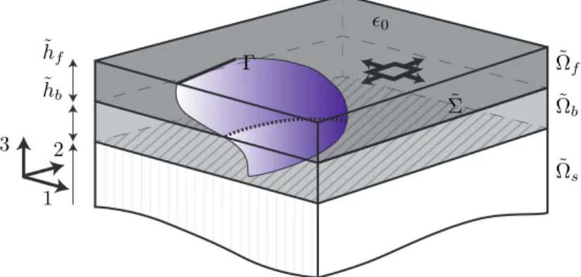
The three-dimensional model system is sketched in Figure 1. A thin film ˜Ωf = !⇥ (0, hf) is bonded to
a rigid substrate ˜Ωs= !⇥ (−hs,−hb) by means of a bonding layer ˜Ωb = !⇥ [−hb, 0], where ! ⇢ R2 is a
bounded open set with Lipschitz boundary. In all that follows, the subscript b indicates quantities relative to the bonding layer and f to the film. The interface between the latter and the substrate is denoted by ˜
Σ = !⇥ {−hb}. We assume the two layers to be isotropic and linearly elastic, the elasticity tensor being
characterized by two material constants, e.g. the Lam´e parameters (λf, µf) and (λb, µb) respectively for the
coating film and bonding layer. We denote by ˜Ω := ˜Ωf[ ˜Ωb[ ˜Ωsthe full medium composed of the film, the
˜ hf ˜ hb 1 2 3 Γ ✏0 ˜ Σ ˜ Ωf ˜ Ωb ˜ Ωs
Figure 1: The three-dimensional model of the brittle system: a thin film Ωf is bonded to a rigid substrate Ωsvia a bonding
layer Ωb. Crack surfaces are noted Γ.
We consider two types of loading modes. The first is the displacement imposed at the interface ˜Σ by the substrate (Dirichlet boundary condition). We denote it by w : ˜Σ! R3. Considering the substrate infinitely
stiff with respect to the film and bonding layer, the displacement w(˜x) at the interface can be identified as the displacement that the structure would undergo neglecting the presence of the surface coating layers under structural loads. The second load type is an inelastic strain ✏0 : ˜Ωf ! R3⇥3. Physically, it may
rise due to thermal loadings, humidity or drying processes, just to note some of the possible multi-physical couplings that may take place. The inelastic strain ✏0(˜x) is interpreted as the strain that the film and the
bonding layer would undergo if they were free from compatibility constraints. We study the specific case of in-plane loads, i.e. loads for which only the in-plane components (✏0)αβ and (w)αare non-vanishing, and
when the inelastic strains are constant through the thickness of each layer. We choose not to account for all the multi-physical phenomena that may induce shrinking and model both loads as independent given parameters.
We represent cracks by discontinuity surfaces of the displacement field, we denote them by Γ and let them free to appear anywhere inside the body without any a priori geometric restriction. Hence, cracks may be any set Γ⇢ ˜Ω of finite 2-dimensional Hausdorff measure. For clarity, the ones inside the film are denoted by Γf := Γ\ ˜Ωf whereas those inside the bonding layer are Γb := Γ\ ˜Ωb. We assume that the
cracks are created at the expense of a surface energy of Griffith-type, i.e. proportional to the measure of the crack surface by a material constant, the toughness Gc. We define it as follows:
S(Γ) := Z Γ Gc(x) dH2, Gc(x) := ( Gf, if x2 ˜Ωf, Gb, if x2 ˜Ωb, (1) whereH2is the Hausdorff surface measure.
In the framework of three-dimensional linear elasticity, the space of admissible displacements is that of square integrable vector fields with square integrable derivatives, defined on the sound part of the body ˜Ω\Γ and satisfying the boundary condition on the extended domain ˜Ωs, namely:
H1 w( ˜Ω\ Γ; R3) := n v2 H1( ˜Ω \ Γ; R3), v = w on ˜Ω s o . To each admissible field we associate the three-dimensional potential elastic energy:
P(u, Γ) := 12 Z
˜ Ω\Γ
W (✏(u(x))− ✏0(x)) dx (2)
where the elastic energy density W (✏) reads:
In the last expression λ(x) and µ(x) are the piecewise constant elasticity parameters of the non-homogeneous body, namely: (λ, µ)(x) := ( (λf, µf) if x2 ˜Ωf, (λb, µb) if x2 ˜Ωb. (4) Finally, the total energy of the thin film system is the sum of the elastic and the surface energies, namely:
E(u, Γ) := P(u, Γ) + S(Γ). 2.3. Static fracture problem
Following the variational approach to fracture (Francfort and Marigo, 1998; Bourdin et al., 2008), we introduce the following definition of static fracture problem. The label static emphasizes that the solution is sought for a fixed load intensity and crack irreversibility does not play any role.
Problem 1(Static problem for the three-dimensional brittle system). The static three-dimensional problem of brittle thin film systems consists in finding, for a given load intensity (✏0, w), crack sets Γ and (possibly)
discontinuous displacement fields u2 H1
w( ˜Ω\ Γ; R3) that solve the following minimization problem
inf{E(u, Γ) : Γ⇢ ˜Ω, u2 Hw1( ˜Ω\ Γ; R3)}, (5)
i.e. that satisfy the following global minimality condition:
E(u, Γ) E(ˆu, ˆΓ), 8ˆΓ ⇢ ˜Ω, 8ˆu 2 Hw1( ˜Ω\ ˆΓ; R3). (6)
The relevant minimization framework when dealing with Griffith-type surface energies is that of global minimization. With such surface energies, the elastic state is a local minimizer regardless of the loading magnitude (see Chambolle et al., 2007, 2010), so that cracks can never nucleate in a body without strong singularities. In some sense, a pre-existing crack or a geometric singularity on the boundary is required in order to release enough elastic energy to balance increase of surface energy. This issue may be mitigated by the introduction of more refined models, such as cohesive or gradient damage models (see Bourdin et al., 2008; Pham et al., 2011b, and also Section 5.3.).
2.4. Quasi-static evolution problem
Unlike in the static case, irreversibility plays a fundamental role in evolution problems. Upon prescrib-ing a load history, parametrized by a scalar t, the three-dimensional evolution problem for brittle thin film systems consists in finding displacements and crack sets verifying a variational statement under the irre-versibility constraint which forbids self-healing of cracks during the loading process. In the framework of variational fracture mechanics, the energetic formulation of evolution problem falls into the class of rate-independent processes as studied in Mielke (2005). The rate-independence implies that solutions to the evolution problem are stable under a reparametrization of the loading parameter, i.e. solutions are the same regardless of the velocity of the load. In this context we allow ourselves to interpret the arbitrarily increasing loading parameter t as a “time” variable. We focus here in the time-discrete formulation of the problem. The reader can refer to Mielke (2005) for a time-continuous formulation.
Problem 2 (Time-discrete evolution problem for the three-dimensional system). Let 0 = t0 t1 . . .
tN = T be the discretization of the time interval [0, T ] into N time steps. A time-discrete quasi-static
evolution of the displacement field and crack set of the three-dimensional system is a mapping ti7! (ui, Γi)
that, given the initial crack state Γ0 and the loading history (✏i
0, wi), verifies the following global unilateral
minimality conditions8i 2 1, . . . , N:
Γi◆ Γi−1, (7a)
E(ui, Γi)
E(u, Γ) 8Γ with Γi−1✓ Γ ⇢ ˜Ω, 8u 2 H1
wi( ˜Ω\ Γ; R3), with ✏0= ✏i0. (7b)
These conditions are equivalent to require (ui, Γi) to be a solution of the minimization problem
inf{E(u, Γ) : Γi−1✓ Γ ⇢ ˜Ω, u2 H1
In the problem above, the condition (7a) ensures the irreversibility of the fracturing process and prevent crack self-healing, whilst condition (7b) requires the constrained energy minimality of the solution at a given time step among all the admissible competitors. The weak regularity assumption on the crack set (finiteness of the two-dimensional Hausdorff measure) will allow the crack to take complex spatial shapes, branch, intersect and coalesce.
2.5. Scaling hypotheses
A natural “small parameter”, denoted henceforth by ", appears in thin film systems as the ratio between the thickness of the surface coating and its in-plane dimension, say L. In addition, thin film systems often ex-hibit abrupt variations of the material parameters characterizing the material behavior of the different layers, spanning several orders of magnitude. The separation of length scales and the material inhomogeneity ren-ders the numerical solution computationally costly and motivates the derivation of reduced two-dimensional limit models. In order to study the asymptotic behavior of the brittle system we consider a specific scaling law for the elastic and geometric quantities and for the material toughnesses, as functions of the small parameter " = hf/L. Amongst all possible choices, we focus on the case where the layers’ thicknesses hb
and hf are of the same order of magnitude and the bonding layer is more compliant and weaker than the
coating film. We formalize the two hypotheses by the following scaling laws on the geometric and elastic constants:
Hypothesis 1(Scaling law of thicknesses and elastic moduli). Being " := hf
L ⌧ 1 ,
we assume that the thickness of the bonding layer hb scales with " as the thickness of the film hf, and that
the ratio between the elastic constant of the bonding layer and that of the film scales as "2:
hb hf = ⇢h, µb µf = "2⇢µ, λb λf = "2⇢λ (9)
where ⇢h, ⇢λ, ⇢µ are dimensionless coefficients independent of ".
Remark 2.1. Hypothesis 1 can be translated into the assumption that the shear energy of the bonding layer and the membrane energy of the film are of the same order of magnitude. A more general scaling law than (9) reflecting this coupling can be envisaged. However, one can show that the asymptotic elastic limit of the whole class of systems is the same. In this sense, a system satisfying (9) is taken as a representative of the whole class.
Regarding the material toughness, we focus on the interesting case where an interplay between cracking within the film and in the bonding layer takes place, the energy of transverse cracks in the film and the energy of in-plane cracks in the bonding layer being of the same order of magnitude. The former is of order GfhfL and the latter of order GbL2, this hypothesis translates in the following scaling of the material
toughnesses:
Hypothesis 2 (Scaling law of toughnesses). Being " = hf/L, the fracture toughnesses of the film Gf and
of the bonding layer Gb are such that
Gb
Gf
= " ⇢G (10)
3. Reduced Model in Scalar Elasticity
Our goal now is to study the asymptotic behavior " & 0 of a system verifying the geometric and constitutive Hypotheses 1 and 2. We expect a non-trivial coupling between the elastic energies of the layers and the competition between film and bonding layer cracks in order to release the stored elastic energy.
In this section we show a rigorous approximation result in the framework of scalar elasticity, i.e. when the displacement field is a scalar function. Although the case of scalar elasticity has an obvious physical meaning only in the case of two-dimensional domains (anti-plane elasticity), we consider the 3D case. This allows us to get, without any further mathematical burden, a clearer analogy to the full vector–valued problem. We prove that under the scaling hypotheses of Section 2.5, the three-dimensional brittle fracture problem admits a limit two-dimensional representation, providing the geometric characterization of crack surfaces both in the film and in the bonding layer, the shape of the optimal displacement field through the thickness and the two-dimensional limit energy. The result is based on the direct method of the calculus of variations and on Γ-convergence techniques. To make the mathematical argument rigorous, the problem is put into a convenient variational setting by considering displacement fields in the functional space SBV of special functions of bounded variation (see Appendix A), as is classical in free-discontinuity problems Ambrosio et al. (2000). A displacement field u in that space may be discontinuous and have jumps on a set denoted by Juwhich can be identified with the cracks. Outside the jump set, such displacements have an (approximate)
gradient denoted byru, which is essentially the regular part of the differential of u. The reader is referred to Ambrosio et al. (2000) for a precise definition of this space and associated problems.
We formulate the problem on an extended domain ˜Ω = ˜Ωf[ ˜Ωb[ ˜Ωsincluding a portion of the substrate,
say ˜Ωs:= ˜!⇥ (−2hb,−hb). The space of all admissible displacements is given by the space
Cw( ˜Ω) :={˜u 2 SBV (˜Ω) : ˜u = w a.e. in ˜Ωs, andk˜ukL1 M}.
Note that the Dirichlet datum w is a priori only defined at the interface ˜Σ between the substrate and the bonding layer. We implicitly extend it constantly to the whole domain ˜Ω so that, from now on, w is identified to a function on ˜Ω independent of the out of plane variable. Therefore, the boundary condition ˜u = w on ˜
Σ = !⇥ {−hb} is expressed on the whole set of finite volume ˜Ωs. We further assume that every deformation
takes place in a container K which is a compact subset of R3, i.e.k˜uk L1
(Ω) M for some fixed constant
M > 0, and kwkL1
(Ωs) M. The latter hypothesis can be removed at the expense of some additional
technicalities (see Dal Maso et al. (2005)).
3.1. Variational formulation in SBV and rescaling of the energy
In the case of scalar elasticity, the elastic energy density (3) reduces to µε|ru|2. To state the variational
problem in a framework well suited for the mathematical analysis we rewrite the energy functional, defined for admissible displacements in ˜u2 Cw( ˜Ω), in the following form:
˜ Eε(˜u) = µf 2 Z ˜ Ωf |r˜u − ✏0|2d˜x + µb 2 Z ˜ Ωb |r˜u − ✏0|2d˜x + GfH2(Ju˜\ ˜Ωf) + GbH2(J˜u\ ˜Ωb). (11)
As is customary in asymptotic methods (Lions, 1973; Ciarlet, 1997), we apply a change of variables in order to formulate the problem on a domain independent of the small parameter ". The new non-dimensional space variable x is defined by the following anisotropic scaling:
x = (x0, x3) = ✓ ˜ x0,x˜3 " ◆ , with x˜0= (˜x1, ˜x2), x0= (x1, x2).
In the new variables, the film, the bonding layer and the substrate occupy the domains Ωf = !⇥ (0, L),
Ωb= !⇥[−⇢hL, 0] and Ωs:= !⇥(−2⇢hL,−⇢hL), respectively. In that configuration, the new displacement
u is defined by:
and the gradient operator may be decomposed into its dimensionless in-plane and out-of-plane component as follows: r˜u(˜x) = ✓ r0u(x), 1 "@3u(x) ◆ , where r0 = ✓ @ @x1 , @ @x2 ◆ , @3= @ @x3 .
Moreover, denoting respectively by ⌫u˜ and ⌫u the unit normal to the jump sets Ju˜and Ju before and after
the change of variables, the surface measure of Ju˜is written as:
H2(J ˜ u) = Z Ju˜ |⌫˜u| dH2= Z Ju |(" ⌫0 u, ⌫u3)| dH2, where ⌫u0 = (⌫u1, ⌫u2).
Hence, the total energy (up to a multiplicative constant 1/") reads as Eε(u) := ˜ Eε(˜u) " = µf 2 Z Ωf ⇣ |r0u− ✏00|2+ 1 "2(@3u) 2⌘dx + ⇢ µ Z Ωb ⇣ "2|r0u− ✏00|2+ (@3u)2 ⌘ dx ! +Gf Z Ju\Ωf + + + ⇣ ⌫u0, ⌫u3 " ⌘+ + + dH 2+ ⇢ G Z Ju\Ωb |(" ⌫u0, ⌫u3)| dH2 ! . (12)
In the previous expression of the energy we have supposed for simplicity that the inelastic strain is of the form ✏0 = (✏00, 0), where ✏00 2 L2(Ω; R2). Note that this change of variable does not affect the imposed
boundary displacement w since it is independent of the out of plane variable. Identifying w with a function defined only on the plane, we henceforth assume that w2 H1(!)
\ L1(!). Consequently, the rescaled space
of all admissible displacements is:
Cw(Ω) :={u 2 SBV (Ω) : u = w a.e. in Ωs, andkukL1(Ω
f) M}
is independent of ". The static fracture mechanics problem is reformulated as follows.
Problem 3(Static problem for scalar elasticity. Weak formulation). For a given load intensity (✏0, w), find
u2 Cw(Ω) that satisfy the following global minimality condition:
Eε(u) Eε(ˆu), 8ˆu 2 Cw(Ω) (13)
Standard arguments ensure that this problem is well posed for fixed ", in the sense that there exists at least a solution. The result is formalized by the following proposition. For the proof, the reader can refer to Ambrosio et al. (2000).
Proposition 3.1. (Existence of minimizers at fixed ") For each " > 0, ✏0
0 2 L2(!; R2) and w 2 H1(!)\
L1(!), there exists a minimizer
uε2 arg min u2Cw(Ω)
Eε(u).
3.2. Limit model for "! 0
Our aim is to determine a limit functionalE0and an associated minimization problem formulated on the
two-dimensional domain ! that approximates the full three-dimensional problem for small ". This energy will turn out to be finite over a set of kinematically admissible displacements which are invariant in the film with respect to the out-of-plane direction. They will be identified with displacements defined only on the plane ! and spanning the set:
C(!) = {u 2 SBV (!) : kukL1(ω) M}.
Note that the approximate gradient of such displacements is given byru = (r0u, 0), while the jump set is
of the form Ju= Ju0 ⇥ (0, L).
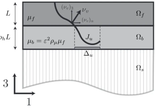
L ⇢hL µf µb= "2⇢µµf Ju ∆u Ωf Ωb Ωs
Figure 2: Rescaled brittle multilayer in scalar elasticity. Cracks are identified by the jump set Juof the admissible displacement
field u 2 SBV (Ωf[ Ωb). Thicknesses, stiffnesses and toughnesses verify a scaling law depending upon the small parameter ε.
Theorem 3.1. For any u2 C(!) let us define: E0(u) := Lµf 2 Z ω|r 0u− ✏0 0|2dx0+ Lµb 2hfhb Z ω\∆u |u − w|2dx0+ LG fH1(Ju0) + LGb hf H 2(∆ u), (14) where ∆u:= ( x02 ! : |u(x0)− w(x0)| > u d:= s 2Gbhb µb ) (15) is the delamination set. Then the energyE0 admits at least one minimizer overC(!) and
min
u2C(ω)E0(u) = limε!0u2Cminw(Ω)E ε(u).
In addition, if uε is a minimizer of Eε overCw(Ω), and uε ! u0 strongly in L2(Ωf) for some u0 2 C(!),
then u0 is a minimizer ofE0 overC(!).
The energy (14) of the limit model can be mechanically interpreted as the energy of a membrane on an elastic foundation `a la Wrinkler undergoing in-plane displacements u 2 C(!). The fracture energies naturally discriminate transverse cracks J0
u and debonded regions ∆u, the former being of codimension 1
while the latter are of codimension 0 in the two-dimensional limit domain !. The debonded regions are explicitly determined by the local threshold criterion (15) on the absolute value of the mismatch between the membrane displacement u and the imposed displacement w on the substrate. The elastic energy density comprises a contribution Lµf
2 |r0u− ✏00|2, a membrane energy, estimating the elastic energy in the film; and
a contribution Lµb 2 |u − w|
2/(h
fhb) due to the interaction with the substrate, estimating the elastic energy
in the bonding layer. The latter contribution is present only in bonded regions !\ ∆u
The proof of Theorem 3.1 is based on a Γ-convergence approach, and its structure is rather classical in dimensional reduction. It rests on three lemmas:
1. Compactness: If (uε) is a sequence with uniformly bounded energyEε, then (up to a subsequence) it
converges strongly in L2(Ω
f) to some u2 C(!);
2. Lower bound : For any u 2 Cw(!) and for any sequence (uε)⇢ Cw(Ω) such that uε ! u strongly in
L2(Ω
f), then
E0(u) lim inf
3. Upper bound (existence of a recovery sequence): For any u2 C(!), there exists a sequence (uε)⇢ Cw(Ω)
such that uε! u strongly in L2(Ωf) and
E0(u)≥ lim sup
ε!0 Eε(uε). (17)
The three previous properties ensure the convergence of minimizers as well as the convergence of the minimal value of the energy. Indeed, the compactness property implies that, if uε is a minimizer ofEεover
Cw(Ω), then a suitable subsequence converges strongly in L2(Ωf) to some u02 C(!), and the lower bound
gives:
E0(u0) lim inf
ε!0 Eε(uε). (18)
On the other hand, if v2 C(!) is a competitor for the reduced two-dimensional problem, the upper bound gives in turn the existence of some recovery sequence (vε)⇢ Cw(Ω) converging strongly in L2(Ωf) to v, and
such that:
E0(v)≥ lim sup ε!0 Eε(vε).
According to the minimality property of uεat fixed ", we infer that:
E0(u0) lim inf
ε!0 Eε(uε) lim supε!0 Eε(uε) lim supε!0 Eε(vε) E0(v),
which ensures that u0 is a minimizer ofE0 overC(!). Taking in particular v = u0 in the previous chains of
inequalities yields:
min
u2Cw(Ω)E
ε(u) =Eε(uε)! E0(u0) = min u2C(ω)E0(u)
which gives the convergence of the minimal value.
For the sake of conciseness and in order not to distract the readers not interested in the mathematical developments, we postpone the rigorous proofs of the above three lemmas to Appendix B. We report below some comments on the key features of the limit behavior of the system that are revealed by the mathematical analysis.
• Requiring the energy of the three-dimensional model (12) to be bounded as " ! 0 implies that the terms @3u and ⌫u3must vanish in the film Ωf. Hence, in the limit "! 0 the displacements are expected
to be constant through the thickness of the film, and the cracks in the film are purely transverse and span its whole thickness. This reasoning is made rigorous in the proof of the compactness property in Section Appendix B.1.
• The scaling hypotheses of Section 2.5 imply that the energy contributions associated to in-plane deformations in the film, through-the-thickness shear in the bonding layer, transverse cracks in the film, and in-plane cracks in the bonding layer are of the same order in " in (12). This entails the emergence of an interesting coupled problem involving all these phenomena, which is the one caught by the limit energy (14).
• In the energy (12) the elastic energy density associated to the in-plane gradient of the displacement inside the bonding layer Ωb is proportional to "2, and thus vanishing for " ! 0. This fact implies
that in the limit "! 0 these gradients may possibly diverge. From a mathematical point of view, it translates into a lack of compactness inside the bonding layer. However, the displacement within the bonding layer is controlled by the imposed displacement on the interface with the substrate (Dirichlet boundary condition) and by the displacement of the film thanks to the continuity at the interface. • The recovery sequence used in the proof of the upper bound (17) gives a deeper insight on the way in
which the limit two-dimensional model approximates the three-dimensional system. Given a membrane displacement u2 C(!), this recovery sequence gives an optimal displacement field defined on the three-dimensional domain Ω to minimize the total energyEεin the limit "! 0. Its full expression is given
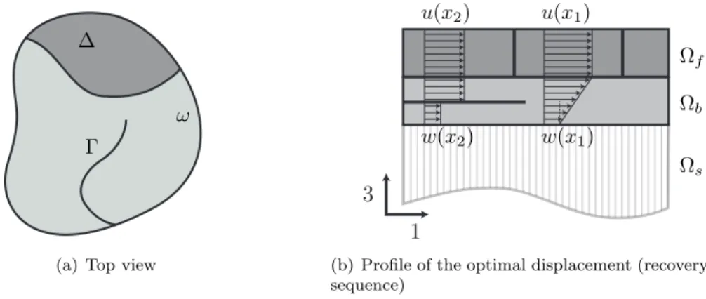
in (B.10). Figure 3(b) sketches the through the thickness distribution of this displacement field and the associated crack sets. In bonded regions, displacements are constant through the thickness of the film and affine within the bonding layer, varying from the boundary condition on Σ to the value of the displacement of the film. In debonded regions no compatibility between the substrate and the film is enforced, hence the film is free to accommodate the inelastic strain.
! Γ
∆
(a) Top view
Ωf Ωb Ωs u(x2) w(x2) u(x1) w(x1)
(b) Profile of the optimal displacement (recovery sequence)
Figure 3: In the limit two-dimensional body ω, transverse cracks Γ and debonded regions ∆ are naturally discriminated, as shown in subfigure (a). Their nucleation and evolution under imposed loads is ruled by the variational principle. The recovery sequence used in the Γ-convergence giving an optimal through-the-thickness distribution of the displacement field is sketched in subfigure 3(b) at points in bonded (x1) and debonded (x2) regions.
4. Reduced model for two-dimensional vectorial elasticity
The results of the previous section concern the case of scalar elasticity. Obviously, the physically relevant setting is that of vectorial elasticity, in which the displacement field is a vector. In this case, the rigorous asymptotic deduction of the limit two-dimensional brittle model involves further technical difficulties from the mathematical point of view. Here we proceed by induction and transpose (without proof) the results of the preceding section in the vectorial setting. In particular, we retain the form of the limit elastic energy, as the sum of the membrane energy of the film and the elastic foundation estimating the energy of the bonding layer; the geometric characterization of the crack surfaces and of the surface energy, naturally decoupling the two fracture modes, as the sum of the contributions due to transverse fracture and debonding. Currently, we are able to provide a full proof (not reported here) of this limit model only in the purely elastic case without fractures. As in Section 2, we formulate the problem in a strong form, i.e. without resorting to the use of functional spaces which allow for arbitrary discontinuities (the space SBD of special functions of bounded deformation, the vectorial generalization of SBV ). In the present context, this choice is mainly formal because we do not report on the mathematical analysis in the vectorial case.
4.1. The reduced limit energy in two-dimensional elasticity
We consider a two-dimensional brittle elastic membrane occupying the domain ! ⇢ R2. In analogy to
the scalar case, we discriminate between transverse cracks Γ and debonded regions ∆. In two dimensions, the former are a subdomain of ! of codimension 1 whereas the latter are a subdomain of codimension 0. We assume that the membrane undergoes only in-plane displacements u = (u1, u2) and that the displacement
field is regular on the crack-free domain !\ Γ. The space of admissible displacements is: H1(!\ Γ; R2).
In analogy with the reduced elastic energy (14) for the scalar case, given the loading as an inelastic isotropic strain ✏02 L2(!; R2⇥2) and an imposed displacement of the substrate w2 H1(!; R2)\L1(!; R2),
the elastic energy of the two-dimensional limit model for the vectorial case is taken as follows: P (u, Γ, ∆) := 1 2 Z ω\Γ A(✏(u)− ✏0)· (✏(u) − ✏0) dx + 1 2 Z ω\∆ µb hb|u − w| 2dx, (19)
where A is the fourth-order tensor representing the isotropic stress-strain relation for the film as a two-dimensional membrane in plane-strain. It is defined by:
A ✏ := hf λfµf
λf+ 2µf
(tr ✏)I2+ 2µfhf✏ (20)
where I2 is the two-dimensional identity tensor. The second integral in the potential energy (19) accounts
for the presence of the bonding layer as an elastic foundation. The surface energy is assumed to be the sum of the contributions given by the transverse cracks Γ and the debonded regions ∆:
S(Γ, ∆) := hfGfH1(Γ) + GbH2(∆). (21)
Hence, the total energy of the two dimensional model is:
E(u, Γ, ∆) := P (u, Γ, ∆) + S(Γ, ∆). (22)
Remark 4.1. Equation (19) is the energy of a linear elastic prestressed plate undergoing purely in-plane displacements plus the energy of a linear elastic foundation in the bonded regions. In the purely elastic case (i.e. when Γ = ∆ =;), for the scaling hypotheses (9) and the assumed in-plane loading, the elastic energy (19) can be obtained as an asymptotic limit for "! 0 of the elastic energy of the three dimensional system introduced in Section 2. The problem is much more difficult in the brittle case because of the technicalities related to the handling of vectorial fields in free discontinuity problems.
4.2. Nondimensionalization and free parameters
Introducing the non-dimensional space variable and displacement field defined by x⇤= x/x
0, u⇤=
u− w pGfx0/µf
, (23)
the total energy (22) may be rewritten in the following non-dimensional form:
E⇤(u⇤, Γ⇤, ∆⇤) =1 2 Z ω⇤ \Γ⇤ A⇤(✏⇤(u⇤)− ✏0⇤)· (✏⇤(u⇤)− ✏0⇤) dx⇤+ 1 2 Z ω⇤ \∆⇤ |u⇤|2dx⇤ +H1(Γ⇤) + γH2(∆⇤), (24) where E⇤= E hfGfx0, A ⇤= A µfhf, ✏ ⇤ =rµfx0 Gf ✏, ✏ ⇤ 0= rµ fx0 Gf (✏0+ ✏(w)) (25) and = µb µf x2 0 hfhb , γ = Gb Gf x0 hf . (26)
Henceforth we consider the total energy in this form dropping the superscripted⇤for the sake of
concise-ness. We conclude from this dimensional analysis that the non-dimensional parameters that fully characterize the energy are:
• The loading parameter ✏⇤
0, which absorbs the imposed displacement of the substrate and models both
loading modes;
• The relative stiffness of the bonding layer and the film ;
• The debonding to transverse cracking relative fracture toughness γ;
• The Poisson ratio ⌫f of the film, that uniquely identifies the non-dimensional stiffness tensor A⇤.
Note that one can always choose the scaling length x0=phfhbµf/µb in order to have = 1. However
in that case the dimension of the domain (in x0-units) will be an additional parameter. In the following we
will adopt the opposite point of view, setting x0 such that the diameter of the domain !⇤ is 1 and keeping
as a free parameter. Note also that the competition between the membrane and the elastic foundation energies entails the existence of a non-dimensional internal characteristic length scale `e:= −1/2, measuring
the decay of the elastic perturbations on the displacement field.
4.3. Problem formulation
We formulate below the static problem and the discrete-in-time evolution problem for the reduced model by extending those of Sections 2.3-2.4 to include the presence of the two fracture modes given by transverse and debonding cracks.
Problem 4 (Static solution of the reduced model). Given a loading ✏0, find u 2 H1(!\ Γ; R2), Γ ⇢ !,
∆✓ ! such that
E(u, Γ, ∆) E(ˆu, ˆΓ, ˆ∆), 8ˆΓ ⇢ !, 8 ˆ∆✓ !, 8ˆu 2 H1(!\ ˆΓ; R2). (27) This condition is equivalent to require that (u, Γ, ∆) solve the following minimization problem
inf{E(u, Γ, ∆) : Γ⇢ !, ∆ ✓ !, u 2 H1(!
\ ˆΓ; R2)
}. (28)
Remark 4.2. As done in the case of scalar elasticity, for any admissible u, one can find explicitly the optimal debonded set by solving a linear optimization problem for the characteristic function χ∆ of the
domain ∆, see Theorem 3.1, which gives: ∆u:= ( x2 ! : |u(x)| > ud:= r 2γ ) . (29)
Hence the static problem may be alternatively reformulated as the minimization of the energy E(u, Γ) := Z ω\Γ 1 2A(✏(u(x))− ✏0)· (✏(u) − ✏0) dx +H 1(Γ) +Z ω\∆u 2|u| 2dx +Z ∆u γ dx (30)
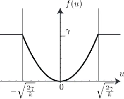
In Equation (30), the energy density due to the film is a quadratic function of the the mismatch between the geometric strains ✏(u) and inelastic strains ✏0. On the other hand the energy density due to the bonding
layer, say f , is quadratic in u (f (u) = |u|2/2) before debonding (
|u| uc) and constant (f (u) = γ) after
debonding. Its dependence on u is sketched in Figure 4. Even in the case without transverse cracks, the total elastic energy E(u,;) is non-linear, non-smooth and non-convex with respect to u. As a consequence of the lack of convexity, we expect lack of uniqueness of the displacement solution as soon as debonding is triggered, even without considering transverse cracks. This problem has been studied is detail in the one-dimensional case in Le´on Baldelli et al. (2013).
Problem 5 (Time-discrete evolution of the reduced model). Let 0 = t0 t1 . . . tN = T be the
discretization of the time interval [0, T ] into N time steps. A time-discrete quasi-static evolution for the dis-placement field and crack set of the reduced two-dimensional model is a mapping ti7! (ui, Γi, ∆i) that, given
f (u) −γ 0 −q2γk q 2γ k u
Figure 4: Qualitative properties of the energy density of the reduced model. The total energy density in the film is quadratic with respect to u in the elastic phase and constant after debonding, see Eqn. (30).
the initial crack state (Γ0, ∆0) and the loading history ✏i
0, verifies the following global unilateral minimality
conditions8i 2 1, . . . , N:
Γi◆ Γi−1, ∆i◆ ∆i−1, (31a)
E(ui, Γi, ∆i) E(ˆu, ˆΓ, ˆ∆), 8ˆΓ with Γi−1✓ ˆΓ ⇢ !, 8 ˆ∆ with ∆i−1✓ ˆ∆✓ !, 8ˆu 2 H1(!\ ˆΓ; R2). (31b) These conditions are equivalent to require (ui, Γi, ∆i) to be a solution of the minimization problem
inf{E(u, Γ, ∆) : Γi−1✓ Γ ⇢ !, ∆i−1✓ ∆ ✓ !, u 2 H1(!
\ Γ; R2)
}. (32)
5. Regularized formulation and implementation
This section details the numerical strategy followed to solve the quasi-static evolution problem for the reduced model presented in Section 4. It relies on the approximation by the means of elliptic functionals of the free discontinuity problem, as originally proposed in Ambrosio and Tortorelli (1990, 1992) for the Mumford-Shah functional (Mumford and Shah, 1989) in the field of image segmentation and exploited in Bourdin et al. (2008) in the framework of variational fracture mechanics.
5.1. Regularized Formulation
The solution of the quasi-static evolution of Problem 5 requires to minimize the energy with respect to the displacement field u, the debonded domain ∆ and the crack set Γ, on which the displacement itself can be discontinuous. Resolving directly this kind of free-discontinuity problem is a major issue, because of the difficulty of the numerical treatment of the unknown crack set. The presence of the irreversibility condition, a unilateral constraint on the crack sets, further complicates the problem. As is now classical in variational fracture mechanics (Bourdin et al., 2008), we adopt here a regularized approach, in which the original problem is approximated by the minimization of a new functional where the transverse cracks Γ are replaced by the localization of a smooth scalar field ↵(x) : x2 ! ! [0, 1], taking the value 0 at sound points and 1 along cracks. The regularization of the energy functional (24) reads:
Eη(u, ↵, ∆) := 1 2 Z ω a(↵)A(✏(u)− ✏0)· (✏(u) − ✏0) dx + 1 2 Z ω |u|2(1− χ∆) dx + cw Z ω ✓ w(↵) ⌘ + ⌘|r 0↵|2 ◆ dx + Z ω γ χ∆dx (33)
where χ∆ is the characteristic function of the debonded domain ∆, ⌘ is a scalar parameter,
a(↵) = (1− ↵)2+ kη, w(↵) = ↵, (34)
and cw= 1/(4R 1
0 pw(↵)d↵) = 3/8 is a normalization constant whose value is set to associate the transverse
1998; Pham et al., 2011a). In the expression (34) for a(↵), the constant kη⌧ ⌘ is a small residual stiffness
required to ensure the regularity of the solutions when ↵ reaches 1.
The solution of the static problem formulated in the Problem 4 is approximated by
min{Eη(u, ↵, ∆) : u2 H1(!; R2), ↵2 H1(!), 0 ↵ 1, ∆ ✓ !} (35)
For ⌘! 0 the solutions of (35) tend to the solutions of (24) in the sense of Γ-convergence1. This implies the
term by term convergence of (33) to (24). In particular, the first integral of (33) approximates the elastic energy of the cracked film given by the first term of (24) and the second integral approximates the total transverse crack length given by the second term of (24). Note that regularization is performed only on transverse cracks Γ since debonding cracks ∆ are explicitely determined in the asymptotic process and do not induce discontinuities on the limit two-dimensional displacements. The advantages of using w(↵) = ↵, instead of w(↵) = ↵2as in Bourdin et al. (2000), are explained in some detail in Pham et al. (2011a). For
quasi-static evolutions, the solutions of Problem 5 are approximated by formulating at each time step tithe
constrained minimization problem:
min{Eη(u, ↵, ∆) : u2 H1(!; R2), ↵2 H1(!), 0 ↵i−1 ↵ 1, ∆i−1✓ ∆ ✓ !} (36)
The proof of the convergence of the evolution problems is proved in Giacomini (2005) for the case of scalar elasticity, assuming that at each time one performs a global minimization of the regularized energy. 5.2. Implementation
Solving numerically the global minimization problem (36) for systems with a large number of degrees of freedom is not a viable option for the current state of the art in optimization methods. Motivated also by the physical considerations that will be detailed in the next subsection, we instead determine at each time ti a solution ui 2 H1(!; R2), ↵i (≥ ↵i−1)2 H1(!), ∆i−1✓ ∆ ✓ ! verifying only the associated first order
(local) optimality conditions. Denoting by
DfF (f )( ˆf ) := d dhF (f + h ˆf ) + + + +h=0 (37) the directional derivative of the functional F with respect to the function f in the direction ˆf , these conditions give the following system of coupled variational problems:
u−problem: DuEη(u, ↵, ∆)(ˆu) = 0, 8ˆu 2 H1(!; R2) (38a)
∆−problem: D∆Eη(u, ↵, ∆)( ˆ∆− ∆) ≥ 0, 8 ˆ∆◆ ∆i−1 (38b)
↵−problem: DαEη(u, ↵, ∆)( ˆ↵− ↵) ≥ 0, 8ˆ↵2 H1(!), ˆ↵≥ ↵i−1 (38c)
where
DuEη(u, ↵, ∆)(ˆu) =
Z
ω
(a(↵)A(✏(u)− ✏0)· ✏(ˆu) + u · ˆu (1 − χ∆)) dx (39a)
D∆Eη(u, ↵, ∆)( ˆ∆) = Z ω ⇣ γ− 2|u| 2⌘χ ˆ ∆dx (39b) DαEη(u, ↵, ∆)( ˆ↵) = Z ω ✓✓ da d↵(↵)A(✏(u)− ✏0)· (✏(u) − ✏0) + cw ⌘ dw d↵(↵) ◆ ˆ ↵+ cw⌘r↵ · rˆ↵ ◆ dx (39c)
1 The rigorous proof of this statement is omitted in the present paper for the sake of conciseness. The convergence without
substrate energy (∆ = ;, κ = 0) and w(α) = α2 is proven in Chambolle (2004). The statement can be trivially adapted to the
case ∆ 6= ;, κ 6= 0) observing that the additional terms are nothing but a continuous perturbation of the functional considered in Chambolle (2004) with respect to which the Γ-convergence (see e.g. Braides (1998)). The extension to more general energies including the case w(α) = α is done in Braides (1998) for scalar elasticity and can be generalized without major issues to vectorial elasticity. Note also that, up to the debonding effect, the energy functional (24) is equivalent (at fixed elasticity) to a vectorial Mumford-Shah functional Mumford and Shah (1989), where the role of the “fidelity term” is played here by the elastic foundation.
To solve this system at each time-step we extend to the present three-field case the alternate minimiza-tions algorithm proposed by Bourdin et al. (2000). We solve iteratively each subproblem with respect to the corresponding field, leaving the other two fixed to the previously available values. More precisely we first solve in this way the u− ∆ subproblem until convergence at fixed ↵ and then iterate solving the ↵-problem (see Algorithm 1). The u problem at fixed ↵ and ∆ is a linear variational equation, which, after space-discretization, we solve using standard iterative Krylov Subspace Solvers. Considering the irreversibility condition on the debonding set, the condition (38b) simply gives χ∆(x) = 1 if the displacement passes a
given threshold at the point x. On the other hand, the ↵-problem at fixed u and ∆ is a linear variational inequality, which we solve using the bound-constrained Newton Trust-Region solver provided in the opti-mization toolbox TAO (Munson et al., 2012). Parallel data representation and linear algebra are based on the PETSc toolkit (Balay et al., 2012). On the other hand the solution of the problem (38b) at fixed u is explicit and local in space.
We do not need any special treatment for the discretization of the computational domain. An un-structured conforming triangulation of the reference domain is obtained by a Delaunay algorithm and the discretization of the fields is done by standard triangular finite elements of classP1 on the fixed mesh. The
discrete fields are subscripted by an h referring to the average diameter of the triangulation. The parameter ⌘controls the width of the localization band of the fracture field, which is of the same order of magnitude of ⌘. The computational mesh is uniformly fine (the mesh is such that h⌧ ⌘) in order to capture and represent the steep gradients within the localization band. A coarse mesh produces a systematic overestimation of the dissipated surface energy.
1 Init: u0, ↵0, χ0 0, tol = 10−4 ; /* sound, unloaded */
2 fori = 1 : n do
3 ui, ↵i, χi ui−1, ↵i−1, χi−1 ; /* Initial guess with solution at previous TS */
4 ↵old
i ↵i;
5 repeat /* Alternate minimizations */
6 χold
i χi ;
7 repeat /* Solve for (u, χ) */
8 ui solution of (38a) with ↵ = ↵i, χ = χi ; /* linear elastic solver */
9 χi χ
i−1;
10 χi(x) 1 if |ui(x)| > uc /* debonding to satisfy (38b) with ↵ = ↵i */ 11 errχ= sup(χi− χold
i );
12 χold
i χi 13 untilerrχ = 0;
14 ↵i solution of (38c) with u = ui, χ = χi; /* Solve for ↵ (constrained solver) */ 15 errα=k↵i− ↵old
i k1;
16 ↵old
i ↵i 17 untilerrα tol; 18 end
Algorithm 1:Algorithm for the solution of the quasi-static time-discrete evolution problem with trans-verse fracture and debonding. At each minimization in (u,χ) and ↵ are performed at each time step, until convergence. For the sake of conciseness, we replace here χ∆by χ.
5.3. Mechanical interpretation of the regularized model with local minimization
The regularized energy (33) falls within the class of the Ambrosio-Tortorelli approximations of free discontinuity problems and is an instance of the gradient damage functional studied in (Pham et al., 2011a,b; Pham and Marigo, 2012). Indeed, the functions w(↵) and a(↵), besides satisfying the hypotheses underlying the Γ-convergence result (see Braides (1998)), verify the additional constitutive assumptions that allow us to identify a(↵) as a stiffness function, w(↵) as a dissipation function, and ↵ as a damage field (Pham et al., 2011b). In this framework, the parameter ⌘ becomes the internal characteristic length of the damage model,
and it has to be thought of as a material parameter. The evolutions associated to the computed solutions of (36), numerically obtained enforcing the first order necessary optimality conditions (38), are consistent with the notion of irreversible evolution of energetically stable states, i.e. of unilateral local minimizers of the total energy. In this sense, transitions between states take place in correspondence to the loss of stability of the current state. Although a study of the stability properties of the energy E(u, ↵, ∆) of Equation (33) depending upon the parameters (, ⌫, γ, ⌘) is beyond the scope of this work, we provide an interpretation of the critical loads in the one-dimensional traction test of a slender strip in Section 6.1. Denoting by σ = a(↵)A (✏(u)− ✏0) the (dimensionless) stress tensor in the film, equation (38c) implies that an elastic
state where ↵ = 0 is admissible only if
A−1σ· σ 3 8⌘(1 + kη)
. (40)
The inequality above gives an explicit relation between the internal length ⌘ and the elastic limit stress σc
in the film, showing that σc/ 1/p⌘.
6. Numerical Experiments
We perform three sets of numerical experiments to illustrate the capabilities of the formulation in simple cases. We focus on the cases of multiple cracking and possible debonding of a slender strip, of a disk and on cracking of a geometrically complex domain. The first set of experiments is also intended to verify the numerical code against the closed form solutions presented in Le´on Baldelli et al. (2013). The second set of experiments shows the capability of capturing geometrically complex two-dimensional crack patterns. Lastly, the third experiment provides a qualitative comparison with a real-life example inspired by the multiple cracking of a vinyl lettering panel.
In what follows, we consider the systems loaded by an inelastic isotropic strain ✏0= tI2increasing linearly
with time.
6.1. Multiple cracking and debonding of a slender strip
We perform a set of verification experiments for the problem of multifissuration and delamination of a one-dimensional stiff film bonded to a substrate. Let us consider a slender brittle elastic body, its reference domain being ! : {x 2 [0, x0L]⇥ [0, x0a]}, with a ⌧ L. To get an exact reference solution, the problem
may be conveniently approximated by the one-dimensional model considered in Le´on Baldelli et al. (2013), provided that a ⌧ `e, `e = −1/2 being the characteristic length of the elastic problem. The condition
a⌧ `e implies that the stress field, under an equi-biaxial imposed inelastic strain, is essentially uniaxial.
The computational domain is of unit length and height a = 2· 10−2, it consists of approximately 7· 103
degrees of freedom. The average mesh size is h = 2· 10−3, the value of ⌘ = 2· 10−2 is held fixed for the
three experiments, the ratio ⌘/h is 10 and the quasi-static simulation consider loading multipliers up to Tmax = 11. Note that as long as ⌘ ⌧ `e no coupling arises at the length scale of ⌘ between the damage
localization bands and the elastic displacement field, which varies over a length scale of order `e.
We perform numerical experiments based on the closed form evolutions reported in Le´on Baldelli et al. (2013). The analytical computation in the latter work is obtained by a global minimization statement, whereas the numerically computed solutions presented here satisfy only first order local optimality conditions and may not be global minimizers.
Transverse fracture experiment. In Figure 5 we represent the outcome of a transverse fracture experiment. The non-dimensional parameters characterizing the experiment are: = 36.0 and γ = 10· 104. The chosen
stiffness ratio corresponds to an internal characteristic elastic length scale `e= 1/6, hence ⌘/`e= 0.12.
The sound elastic energy branch loses stability at t = 4.81, see Figure 5(c), when the system jumps towards the cracked state with one transverse crack in the center of the domain. This releases elastic energy at the expense of the surface energy, as it can be seen in the energy chart in Figure 5(c). As the load increases further, the system undergoes the elastic loading phase of the two segments. At t = 7.46 the loss of stability
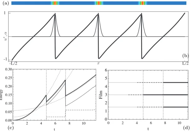
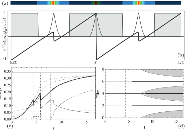
1 -1 -L/2 L/2 0 1 2 3 4 0 2 4 6 8 10 12 14 t E ne rgy 0 2 4 6 8 10 0.00 0.05 0.10 0.15 0.20 0.25 0.30 t E ne rgy 0 1 2 3 4 5 6 t F il m 0 2 4 6 8 10 1 -1 -L/2 L/2 (a) (b) (d) (c)
Figure 5: Top: snapshot of the fracture field at t = Tmax for the perfectly bonded transverse fracture experiment. Cracks
are equidistributed and represented by the localization of the damage field α. The values of α 2 [0, 1] are mapped onto a “inverted-hot” color table, blue corresponding to α = 0 (sound material), red corresponding to α = 1 (fully developed fracture). Middle: displacement and fracture field along the axis [−L/2, L/2] ⇥ {0} for t = Tmax. The displacement field
u∗
(x) = u(x)/ maxx∈ωu(x) is normalized and displayed with a thick solid line. The fracture field α is shown with a thin black
stroke. Bottom: in the energy chart (left) the total energy is plotted in bold line, the energy transverse fracture energy with a dashed line and the elastic energy with a thin solid line. Grid lines indicate the critic loads for transverse cracking. The total energy of the closed form solutions reported in Le´on Baldelli et al. (2013) is plotted with a dotted line. In the space-time evolution diagram (right), the domain ω is represented on the vertical axis and the load on the horizontal axis. Solid black horizontal lines indicate the position of cracks during the evolution.
of this solution leads to the appearance of two add-cracks, each at the middle of the segments. The snapshot of the last loading step is shown in Figure 5(a) and the profile of the displacement and fracture fields are shown in Figure 5(b). The computed energy branches are seamlessly superposed to the analytical ones, and the evolution of the system is illustrated by the space-time chart in Figure 5(d). Critical times at which cracking happens differ between the numerical experience and the analytic computation, due to the global vs. local setting of minimization. As expected, the critical loads corresponding to the local minimization criterion systematically overestimate those satisfying the global criterion.
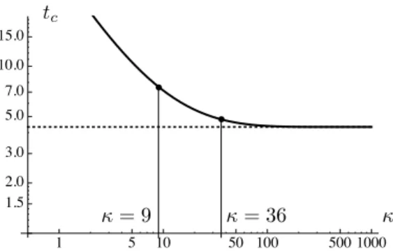
Ê Ê 1 5 10 50 100 500 1000 10.0 5.0 2.0 3.0 1.5 15.0 7.0 tc = 9 = 36
Figure 6: Critical loads of the transverse fracture experiments are compared to the elastic limit (Equation (40)) computed with the stability condition (38c) and plotted against the relative stiffness κ. The plot is for η = 0.02. The asymptote κ ! 1 corresponds to the limit case of a long film with homogeneous stress. For κ ! 0 the critic load tc! 1, this corresponds to the
limit case of system in which no energy is stored in the bonding layer and the film freely accommodates the inelastic strain.
The critical fracture loads are interpreted under the light of the considerations sketched in Section 5.3. Using a one-dimensional model, the critical loading for leaving the purely elastic regime may be established analytically, using Equation (40). Indeed, for the elastic solution (↵ = 0), the stress σ as a function of the loading may be easily computed analytically (see Le´on Baldelli et al., 2013). Substituting this expression into Equation (40), one finds that purely elastic solutions are admissible for loadings not greater than
tc(, ⌘) := p3/8 p⌘ (1 + kη) 1 ⇣ 1− sech⇣p2κ⌘⌘ . (41)
The critical time for the elastic solution is plotted in Figure 6.1 as a function of the stiffness ratio for ⌘ = 0.02. It is a monotonic function of decreasing from +1 for ! 0+ top3/8 ⌘(1 + k
η) for ! 1.
In the same figure, we display with black dots the critical load captured by the numerical experiment. The first transverse fracture appears for the strip of stiffness ratio = 36.0 for t = 4.81. It creates two uncracked strips of half-length that, recalling the definition of , have an equivalent stiffness ratio /4 = 9. Both these two strips further break into two parts at the second critical load t = 7.46. Both critical loads coincide, within a small error, with the critical loads of the elastic solution given by equation (41) for equal to 36 and 9, respectively (see Figure 6.1). Indeed, as done in (Pham et al., 2011b) for the case of a bar in traction, it may be shown that for sufficiently long strips the elastic limit also coincides with the stability limit of the solution without damage localizations (i.e. fractures). When passing this limit, the fundamental undamaged solution becomes unstable. The numerical algorithm based on alternate minimizations detects new descent directions and automatically jumps to a new (stable) solution branch, implying newly added cracks. Note that after the first transverse crack, the first order stability properties of the two cracked segments are almost insensitive of the half localizations at the boundaries. This does not hold asymptotically when inducing further fragmentations, upon increasing the load and producing small segments whose characteristic elastic length is comparable to the internal length ⌘ associated to the damage localization. This regime is not explored in the present work, in all the experiments the internal length of the damage process ⌘ is kept smaller than the elastic length `e= −1/2.
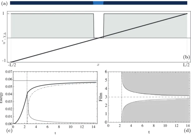
Debonding experiment. Figure 7 refers to a debonding experiment with the same equivalent stiffness = 36.0 as the experiment above (and hence the same elastic length `e = 1/6) and a lower toughness ratio
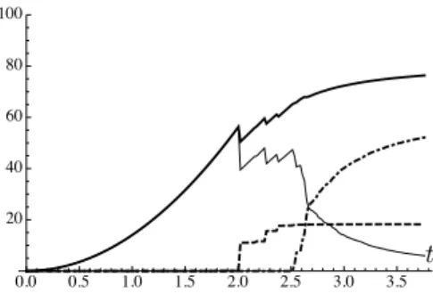
γ= 0.50. The sound elastic bonded branch is followed by the debonding phase, whose onset is at t = 2.25. Elastic energy is released at the expense of the debonding surface energy. The total energy asymptotically approaches the limit of the energy of the completely debonded film E1 = Lγ. The computed energy coincide with the analytical energies and also the evolution are identical. In fact, differently from the perfectly bonded transverse cracking experiment, both in the numerical and closed form computations, the evolution of debonding relies only on first order optimality conditions Le´on Baldelli et al. (2013). A snapshot of the last time step is displayed in Figure 7(a) and the displacement and debonding fields in Figure 7(b).
0 1 2 3 4 5 6 t F il m 0 2 4 6 8 10 12 14 0 2 4 6 8 10 12 14 0.00 0.01 0.02 0.03 0.04 0.05 0.06 0.07 t E ne rgy 1 -1 -L/2 L/2 (a) (b) (d) (c)
Figure 7: Top: Fracture and debonding fields at t = Tmax for the deboonding experiment. Debonding (χ∆(x) = 1 is the
darker area) is symmetric about the two axes. Middle: The characteristic function of the debonded domain is shaded gray, displacement is plotted with a thick stroke. Note that, in debonded regions, the displacement in linear and accommodates the imposed strain. Bottom: energy chart (left) and evolution diagram (right). Debonding onset and its evolution coincide in both numeric and analytic computations as they are derived as consequences of the first order necessary condition for energy optimality. The thin black line in the space-time evolution plot (right) is the analytical solution to the debonding problem obtained in Le´on Baldelli et al. (2013).
The debonded domain is symmetric with respect to the axes of the film. In the debonded domain, the displacement is linear and accommodates the imposed inelastic strain, hence the energy vanishes. We remark that in spite of the lack of uniqueness of the displacement field in the debonded solution (recall that all states with equal debonded length have equal energy, irrespective of the location of the debonded area), numerical computations seem to favor symmetric solutions. The space-time chart illustrates the evolution, showing the bonded domain for a given load intensity.
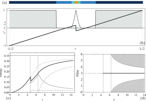
Coupled experiments. Experiments in Figures 8 and 9 show the interplay between the two failure modes. In these two experiments, the system exhibits one (resp. three) transverse cracks prior to peripheral debonding. The evolutions are obtained choosing = 36.0 (`e = 1/6) and γ = 2.2 (resp. = 64.0 and γ = 3.1,
i.e. `e = 1/8). The corresponding energy chart and state diagrams are shown in Figures 8(c) and 9(c).
A higher order effect is observed at the onset of debonding for the second coupled experiment due to the boundary layer induced by the fracture field around the middle crack causing local softening. This breaks the symmetry of the boundary conditions for the two segments. The effect is visible in the space-time evolution and in the debonding and elastic energy terms in Figure 9(d), although not noticeable at the global level of the total energy.
1 -1 -L/2 L/2 0 2 4 6 8 10 12 14 0.00 0.05 0.10 0.15 0.20 0.25 0.30 0.35 t E ne rgy 0 1 2 3 4 5 6 t F il m 0 2 4 6 8 10 12 14 1 -1 -L/2 L/2 (a) (b) (d) (c)
Figure 8: Top: fracture and debonding fields on the reference domain ω at t = Tmax for the first coupled experiment; one
transverse crack in the center and symmetric debonding starting from the boundaries. Middle: a single crack in the center of the film, the symmetric debonded region and the displacement field. Bottom: the analytic solution (global minimization) anticipates the appearance of the crack of the numerical experiment (local minimization). The debonding onset and evolution in both cases are equal.
6.2. Multiple cracking and debonding of a thin disk
We illustrate the ability to capture complex crack geometries and time-evolutions considering the prob-lem of a homogeneously prestressed circular elastic wafer. We analyze qualitatively the outcome of the experiments showing its soundness on a mechanical basis and its coherence with the mechanical intuition and commonly reported experimental observations. The computational domain is of unit diameter, each experiment is univocally identified by four non-dimensional parameters: the relative stiffness , the relative toughness γ, the Poisson ratio ⌫ and the maximum load intensity Tmax.
We introduce a non-homogeneity in order to explore more complex crack patterns around the sound elastic state. In the center of the wafer, we place a domain Dη of size of O(⌘) where we set ↵ = 1, see
Figure 11(a).
Multiple cracking only. The non-dimensional parameters for this experiment are = 200.0 (`e = 0.071),
γ= 4.6, ⌫ = 0.3 and Tmax= 3.76. The wafer undergoes an elastic loading phase during which the domain
!\ Dη remains sound. As the load increases, nucleation is localized in the neighborhood of the domain
Dη. Sudden fracture occurs at t = 2.0: a network of cracks of finite length appears in a single loading step
and a network of hexagonal polygons forms. We observe a non-axisymmetric solution to a problem with axisymmetric data. Away from the boundaries, the cracks are structured in a network of six hexagons all with the same characteristic diameter. We capture the spontaneous nucleation of cracks within the domain, away from possible boundary non-homogeneities, with preference of 2⇡/3-junctions over ⇡/2-junctions. This feature corresponds to regimes in which the sound solution is stable until load intensities high enough to