Decentralized Resource Allocation for Synchronized Tasks
through Adaptive Large Neighborhood Search (ALNS)
by
Christian D. Montgomery
B.S. Computer Engineering and Computer Science United States Naval Academy, 2018
SUBMITTED TO THE DEPARTMENT OF AERONAUTICS AND ASTRONAUTICS IN PARTIAL FULFILLMENT OF THE REQUIREMENTS FOR THE DEGREE OF
MASTER OF SCIENCE IN AERONAUTICS AND ASTRONAUTICS AT THE
MASSACHUSETTS INSTITUTE OF TECHNOLOGY MAY 2020
©2020 Christian D. Montgomery. All rights reserved.
The author hereby grants to MIT permission to reproduce and to distribute publicly paper and electronic copies of this thesis document in whole or in part in any medium now known or
hereafter created.
Signature of Author: ____________________________________________________________ Department of Aeronautics and Astronautics
May 19, 2020 Approved by: __________________________________________________________________
Mark Abramson Principal Member of the Technical Staff The Charles Stark Draper Laboratory, Inc Technical Supervisor Certified by: ___________________________________________________________________
Hamsa Balakrishnan Professor of Aeronautics and Astronautics Thesis Supervisor Accepted by: __________________________________________________________________
Sertac Karaman Professor of Aeronautics and Astronautics Chairman, Committee for Graduate Students
2
Decentralized Resource Allocation for Synchronized Tasks through Adaptive
Large Neighborhood Search (ALNS)
by
Christian D. Montgomery
Submitted to the Department of Aeronautics and Astronautics on May 19, 2020 in partial fulfillment of the
requirements for the degree of
Master of Science in Aeronautics and Astronautics
Abstract
This thesis explores a method for multiple suppliers to coordinate resource scheduling of task requests from multiple consumers using decentralized planning. A time window is
associated with each task and some tasks require simultaneous servicing from multiple resources of specified classes to fulfil a request. The suppliers create schedules for their resources that maximize the value of all tasks fulfilled, while minimizing travel cost, and respecting all time window constraints. This thesis presents Infeasibility Cooling Adaptive Allocation for Resource United Scheduling (ICAARUS), a novel Adaptive Large Neighborhood Search (ALNS)
algorithm that is capable of synchronizing tasks across a variable number of resources. A
supplier’s individual schedule and cost function is kept private from consumers. An e-commerce style of multi-round bidding is introduced to notify suppliers of resource request parameters and to allow consumers to synchronize resources from independent suppliers. A Mixed-Integer Linear Program (MILP) is used by the consumer to select the least costly bids that can be combined to fulfill a task’s requirements.
3
TABLE OF CONTENTS
1
Introduction ... 6
1.1 Thesis Overview ... 6 1.2 Contributions... 7 1.3 Motivation ... 82
Operational Concept ...10
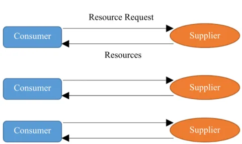
2.1 Consumer-Supplier Relationship ... 102.1.1 One Consumer to One Supplier ... 11
2.1.2 One Consumer to Multiple Suppliers ... 12
2.1.3 Multiple Consumer to Multiple Suppliers... 13
2.2 E-Commerce Bidding Structure ... 14
2.2.1 Incomplete Fulfillment ... 17
2.2.2 Complete Fulfillment ... 18
2.2.3 Unsynchronized Fulfillment ... 19
3
Model Formulation and Development ...22
3.1 Supplier Scheduling Problem (SSP) ... 22
3.1.1 Inputs to Supplier Solver ... 22
3.1.1.1 Supplier Inputs ... 22
3.1.1.2 Task Inputs ... 23
3.1.2 Outputs of Supplier Solver ... 24
3.2 Network Representation... 26
3.2.1 Static Graph Representation ... 26
3.2.2 Time-Space Graph Representation ... 27
3.2.3 Placement-Space Graph Representation ... 28
3.3 Problem Classification ... 29
3.3.1 Mathematical Programming Background ... 30
3.3.2 Travelling Salesman Problem ... 30
3.3.2.1 Mixed Integer Programming Formulation for Traveling Salesman Problem .. 30
3.3.2.2 Exact Solution Methods... 31
3.3.2.3 Heuristic Solution Methods ... 32
3.3.3 Traveling Salesman Problem with Time Windows ... 34
4
3.4 Mixed Integer Linear Programming Model ... 36
3.4.1 Supplier MILP Model Formulation ... 37
3.4.1.1 Set Definitions ... 37 3.4.1.2 Decision Variables ... 37 3.4.1.3 Input Variables ... 38 3.4.1.4 Objective Function ... 38 3.4.1.5 Constraints ... 39 3.4.1.6 Linearization of Constraint ... 40
3.4.2 Maximum Time Window Model Formulation ... 41
3.4.2.1 MTW Objective Function ... 42
3.4.2.2 Maximum Time Window Constraints ... 42
3.4.3 Supplier MILP w/ Synchronization Model Formulation ... 43
3.4.3.1 Synchronization Constraints ... 43
3.4.4 Consumer MILP Model Formulation... 45
3.4.4.1 Set Definitions ... 45 3.4.4.2 Decision Variables ... 45 3.4.4.3 Input Variables ... 46 3.4.4.4 Objective Function ... 46 3.4.4.5 Constraints ... 46 3.5 Implementation ... 47
4
Formulation of Algorithm ...48
4.1 Confirmation Lists ... 49 4.2 Construction Phase... 504.2.1 COPA Construction Phase ... 51
4.2.2 Dual-Collection Construction Phase ... 52
4.2.3 ICAARUS Construction Phase ... 53
4.3 Improvement Phase ... 57
4.3.1 Infeasibility measurement ... 58
4.3.2 Avoiding Cross Synchronization ... 59
4.3.2.1 Checking for Cross Synchronization ... 60
4.3.2.2 Constructing Cross Synchronization Matrix ... 62
5 4.3.3 Removal Methods ... 63 4.3.3.1 Related Removal... 63 4.3.3.2 Worst Removal ... 65 4.3.3.3 Synchronized-Services Removal ... 67 4.3.3.4 Route Removal ... 67 4.3.3.5 Random Removal ... 68 4.3.4 Insertion Methods ... 68 4.3.4.1 Best Insertion ... 69 4.3.4.2 Regret Insertion ... 71
4.3.5 Removal and Insertion Weights ... 71
5
Tests and Analysis ...73
5.1 Test Datasets and Parameters... 73
5.1.1 Test Set Development ... 74
5.1.2 Parameter Selection... 75 5.2 Evaluation Tests ... 75 5.2.1 MILP Comparison... 76 5.2.2 Runtime Comparison ... 77 5.2.3 Optimality Comparison ... 79 5.3 Synchronization Coordination ... 82
6
Conclusion ...84
6.1 Summary of Contributions ... 84 6.2 Future Work ... 856.2.1 Adaptive Drop List... 85
6.2.2 Robust Optimization for Duration Changes ... 87
6.2.3 Robust Optimization for Value Changes ... 89
6
Chapter 1
1
Introduction
Recent advancements in research and technology for robotics has created resources with the ability to operate in a variety of domains. Current operations are unable to take full advantage of disparate capabilities across all domains. Planning of modern day operations are becoming increasingly complex. Challenges ranging from stove piped mission commanders who are only aware of the few resources assigned to them, to rigid schedules that are too complicated to re-plan.
The purpose of this thesis is to develop an algorithm that coordinates resources across multiple domains through decentralized bidding for multiple consumers. This algorithm
addresses two main challenges to planning multi-domain operations as envisioned in the Army in Multi-Domain Operations 2028 [3]. First, to properly manage and fully realize the capabilities of so many decentralized resources, a bidding system is needed. This bidding structure should direct suppliers to service customers that most value resources and require the least cost
expenditure. Second, an algorithm that solves the Supplier Scheduling Problem (SSP) must do so in an operationally feasible runtime. Computing solutions is complicated because of the
synchronization requirements of a single task across multiple resources. Thesis Overview
This thesis presents a method to coordinate and create schedules for multi-domain operations. The development of this method and the associated technical challenges are described in the following six chapters. An overview of the chapters follows:
Chapter 2 – Operational Concept. In this chapter, the concept of e-commerce is introduced as a solution to decentralized resource allocation. The time and spatial operational constraints in the Supplier Scheduling Problem are assumed fixed in this work.
Chapter 3 – Model Formulation and Development. In this chapter, a mathematical model is created for the scope of the SSP. It is shown that this problem can be modeled as a network problem while maintaining the constraints expressed in Chapter 2. Similar problems in
7
past literature are reviewed to lend insight into the development of an algorithm for the SSP. In particular, the Traveling Salesman Problem and extended variants are explored due to their similarity to the SSP. A Mixed-Integer Linear Program (MILP) is introduced for providing optimal solutions for the SSP. An analysis of this method is presented in Chapter 5.
Chapter 4 – Formulation of Algorithm. This chapter formulates the Infeasibility Cooling Adaptive Allocation for Resource United Scheduling (ICAARUS) Algorithm to solve the SSP. This chapter begins with the formulation of the Composite Operations Planning Algorithm (COPA) to solve the UAV Planner Problem. However, the Composite generation algorithm falls short of ensuring resource synchronization across a task. To accomplish this, Adaptive Large Neighborhood Search (ALNS) is studied in the Vehicle Routing Problem, which has synchronization across a single supplier’s resources as a constraint. ICAARUS explores a large region of the state space by allowing infeasible schedules to be created and culled through Simulated Annealing.
Chapter 5 – Tests and Analysis. This chapter covers the testing and analysis of the MILP and ICAARUS. It is shown that while the MILP provides an exact solution, ICAARUS is able to find a feasible schedule in much less time. It is shown that the MILP is unable to scale and solve beyond 20 task requests in a reasonable time manner. Meanwhile ICAARUS is able to produce a schedule for large cases including 40 task requests, in under 30 minutes.
Chapter 6 – Conclusions. This chapter provides a summary of the work and resulting contributions presented in this thesis. Proposals for modifications to our methods are presented, including the incorporation of robust planning into the resource allocation process.
Contributions
This research makes the following contributions:
1. An e-commerce bidding structure to coordinate multiple consumers with multiple suppliers asynchronously in a decentralized manner.
2. A MILP model for suppliers to solve the SSP with synchronization. 3. A MILP model for consumers to select cheapest resource bids.
8
4. The development and implementation of ICAARUS, an algorithm to schedule multiple resources for tasks requiring time and spatial synchronization.
5. Testing and analysis of the supplier MILP and ICAARUS. 6. Recommendations for modifications to ICAARUS.
Motivation
In the summer of 2018 at Rim of the Pacific (RIMPAC), the world’s largest international maritime exercise, the USS Racine underwent a sinking exercise (SINKEX) with a range of military units working together to sink this one ship [1]. Originally the ship was targeted by a P-3 Orion aircraft, but when its ability to communicate targeting information was jammed in the simulation, both a Gray Eagle Unmanned Aerial Vehicle (UAV) and Army AH64E Apache helicopter were able to respond and support targeting through new data-link backups. This re-established communication provided for overwhelming firepower from multiple domains with Naval Strike Missiles and HIMARS artillery launched by the Army, and AGM-84 Harpoon missiles launched by a Navy P-8 aircraft. To finish the exercise, the submarine USS Olympia also launched a MK-48 torpedo to sink the USS Racine. While this SINKEX was carefully orchestrated to coordinate Army and Navy capabilities from the sea, air, and land, it showed the flexibility and capability of multi-domain operations.
This exercise reflects the US Navy’s A Design for Maintaining Maritime Superiority call for Distributed Maritime Operations (DMO), described as aiming to “deepen naval integration with other services to realize [strategy] in multi-domain, distributed operations” [2]. In this thesis, domain refers to the five warfighting areas of sea, land, air, cyber, and space. The US Army calls for Multi-Domain Operations (MDO) to converge all domain capabilities across time and space to inundate adversaries. This convergence is envisioned in Army in Multi-Domain Operations 2028: (1) Create synergy across domains for overlapping redundancy, and (2) give commanders multiple forms of attack through options that are unforeseen by the enemy [3]. Historically the delivery of effects onto an adversary are referred to as “Kill-Chains” with each effect having siloed planning and execution path, this new level of complexity creates the idea of “Kill-Webs, complex representation of effect chains with multiple possible paths” [4]. However, this new capability presents a problem of scalability with “a factorial increase in possible
inter-9
relationships that will test the limits of current analytic approaches” [4]. LCDR Will Spears also remarks that while MDO is the natural evolution of Joint Warfare, communication barriers of information classification levels and technical language discrepancies between disciplines will require a “level of agility that is beyond [current capabilities]” [5]. With this communication though, MG VeraLinn Jamieson describes a vision for the Air Force’s Intelligence, Surveillance, and Reconnaissance (ISR) as “Fusion Warfare,” which “integrates and synchronizes information from multiple sources and domains” to fly, fight, and win in any battlespace [6].
10
Chapter 2
2
Operational Concept
This chapter clarifies what is e-commerce and how it is used in the context of this thesis. Advancements in Information Technology in the 21st century have led to supplying services and commodities through telecommunication networks. Rarely does a student nowadays need to physically go to a bookstore, searching for the best deal on textbooks. Instead a student can virtually specify a book’s title and condition, and then select the cheapest option from a range of suppliers. This is electronic commerce, or e-commerce. The abundance and speed of access, that defines modern day corporations like Amazon or eBay, are characteristics necessary for MDO and thus e-commerce is an appealing tool to future military planners.
Nanehkaran defines e-commerce through three main components: communication systems, data management systems and security [7]. This thesis assumes hardware capabilities for any communication and data management systems are possible, leaving that work to future researchers. This thesis, as mentioned in Chapter 1, focuses on presenting ICAARUS, an algorithm for scheduling resources from suppliers to consumers. This chapter will define the communications between consumers and suppliers, and what data is shared versus what is kept private in the interest of user security.
The market proposed in this thesis makes several assumptions that depart from classical marketplace features. Firstly, consumers and suppliers do not exchange money for services. Consumers express their level of desirability for a task through assigning value. Consumers are assumed to be honest actors, meaning they do not assign high value to low priority tasks for the purpose of cheating resources from suppliers. Suppliers are also assumed to always be willing to service a task request if feasible in their schedule. However, some suppliers are busier than others and express this through costs associated with offered resources.
Consumer-Supplier Relationship
This thesis will focus on how suppliers can more effectively allocate limited resources to consumers. This interaction begins by consumers, who have missions they are planning, creating
11
tasks which require resources. For the purpose of this thesis only consumers generate tasks, and only suppliers have resources, i.e. no supplier is trying to plan a mission and no consumer has resources. These tasks are defined by several parameters which are common questions a commander may need answered when planning a mission:
Value: Assigned number, [1,100], that quantifies the importance of the task. Position: Two-dimensional location at which the task could be performed. Minimum Duration: The time it takes to completely service the task.
Time Window: The start and end time in which the task must be serviced. If a resource arrives before the start of the window, it cannot begin servicing until the early edge of the time window. In addition, if the minimum duration is not fulfilled before the end time, it is too late and the task is not counted as completed. Resources: A task may require one or multiple resources. These resources are defined by
types, so only resource of one type can fulfill that type requested.
For a task to be serviced, all resources must be in the same position for an overlapping minimum duration within that task’s time period.
2.1.1 One Consumer to One Supplier
The simplest case of this scenario is one consumer assigned to one supplier. This
stovepipe relationship is still prevalent today for the ability to 1) simplify scheduling and 2) keep planning details confidential. A consumer can only get resources from one source, so a task’s feasibility is straightforward to find through asking if the one supplier has the requested resources or is pre-occupied with servicing another task. As resources are only servicing one customer, the supplier’s schedule is known to only that consumer.
12
Figure 1: One Consumer to One Supllier
The immediate drawbacks of task planning with this relationship is a consumer’s
complete reliance on one supplier. Any task requiring a resource that the supplier does not have is instantly infeasible with no other options. Also this relationship can be observed by an adversary and become susceptible to attack. An adversary can predict operational actions by noting historical consumer-supplier relationships, even if dedicated supply chains are not published information. An adversary could be aware of a consumer’s immediate actions by observing the movements of its supplier’s resources, or even remove this one supplier to cripple the consumer completely.
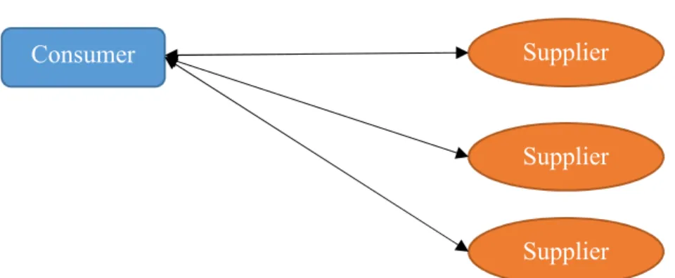
2.1.2 One Consumer to Multiple Suppliers
As the internet opens up connections across the world, so does e-commerce aim to open up connections to suppliers. Through e-commerce comes the ability for a single consumer to expand its network of resource access from one supplier to multiple suppliers.
Consumer Supplier
Resource Request
Resources
Consumer Supplier
13
Figure 2: One Consumer to Multiple Suppliers
This multitude of suppliers is a powerful tool for improving mission planning. Through more suppliers comes greater availability of resources, and thus increased probability of a consumer finding the resources they desire when they are needed. Another operational benefit of this network is unpredictability. Through an abundance of options for planning operations, consumers will naturally begin to vary their supplier choices. This will obscure intended actions to adversaries and remove supplier vulnerabilities through redundancy.
With more nodes in a network comes more potential leaks of information in the system. Some operational scenarios could have mission commanders concerned about adversaries eavesdropping into communications and compromising security. That is why in this thesis, suppliers do not share schedules with each other or consumers. A supplier only responds to the consumer through a “bid” with the following information:
Cost: This is a measure of how much travel time the supplier must expend for its
resources to arrive at the task. Travel time is the expense that is analogous to fuel for resources that are expensive to exercise.
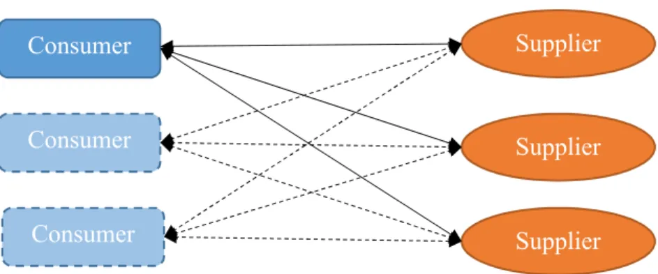
Time Window: The arrival and departure time of resources to the task’s location. Resources: Which resources, type and quantity, are being allocated to the task. 2.1.3 Multiple Consumers to Multiple Suppliers
In theory, multiple suppliers collectively servicing only one consumer would be ideal, but in reality, this system requires multiple consumers. In a finite world, gaining the flexibility of numerous suppliers in a network also requires multiple consumers pooling their supply chains to
Consumer Supplier
Supplier
14
create this network. For e-commerce to be utilized in a practical setting, consumers will need to compete against each other for supplier resources.
Figure 3: Multiple Consumer to Multiple Suppliers
Consumers do not collaborate with other consumers for achieving a global maximum task fulfillment rate. A consumer is concerned with only completing its own tasks. These
self-interested actors will continue to request resources from all suppliers until the task is fulfilled or bidding is stopped. This means suppliers in this network will receive a larger volume of resource requests, compared to suppliers operating in a one consumer to one supplier relationship. For the desired option creation feature of e-commerce, comes inherent complexity for the system to manage.
E-Commerce Bidding Structure
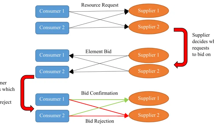
In this thesis, a consumer is responsible for stating what resource types are needed and time range that these resources are needed for a task. The challenge of calculating a path for how those resources will get to the task is removed from the consumer’s concern. Consumers interact with suppliers for resources through multiple bidding rounds. The procedure for each round is a three part handshake: 1) Resource requests are sent from the consumer with the task’s critical information to the supplier; 2) element bids are sent from the supplier to the consumer
expressing resource availability; and 3) bid confirmations are sent from the consumer to the supplier to accept or reject the element bids. Figure 4 illustrates the flow of information in these resource bidding rounds:
Consumer Supplier
Supplier
Supplier Consumer
15
Figure 4: Information Flow in One Bidding Round
After resources are requested, the consumer will receive element bids from suppliers with three distinct outcomes for each task:
1. Incomplete Fulfillment
For at least one resource the task requests, no bids were received. 2. Complete Fulfillment
From one or multiple suppliers all resources a task requested are fulfilled and have an overlapping service time of at least the minimum required duration. 2. Unsynchronized Fulfillment
From multiple suppliers a task receives bids on all resources requested, but the received bids have misaligned service times.
Consumer 1 Consumer 2 Supplier 1 Supplier 2 Resource Request Consumer 1 Consumer 2 Supplier 1 Supplier 2 Element Bid Supplier decides which requests to bid on Consumer 1 Consumer 2 Supplier 1 Supplier 2 Bid Confirmation Bid Rejection Consumer decides which bids to accept/reject
16
These three distinct outcomes require a protocol for handling, with the desired effect that this process would get all tasks to Complete Fulfillment before the end of bidding. MG Jamieson envisions “fusion warfare” of the future as continuously repeating OODA loops for mission planners of ISR operations. The OODA loop is a classic decision-making process distinguished by its four phases of Observe, Orient, Decide, Act. These four phases are the basis of the Consumer Decision Process for this Marketplace:
Observe – Which element bids are received.
Orient – Which fulfillment status does a task fall under. Decide – How to handle these fulfillment statuses.
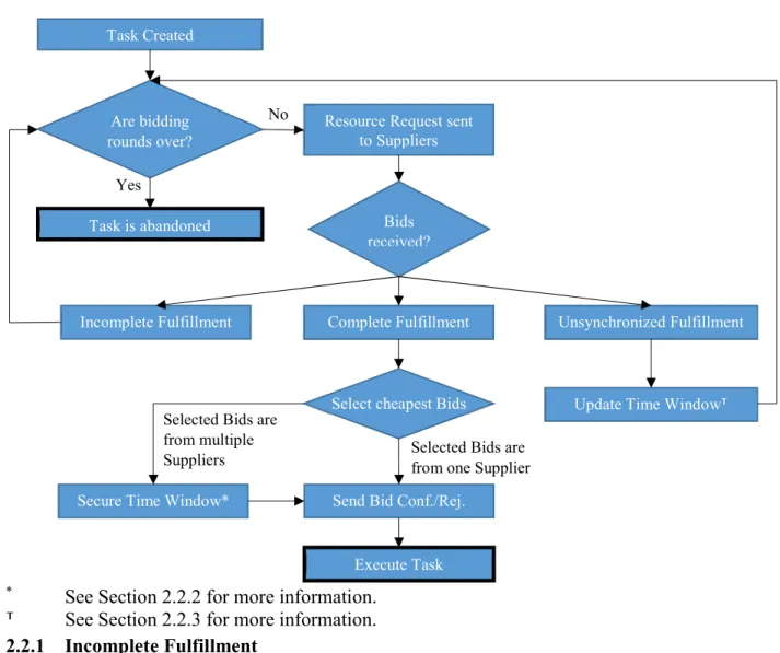
Act – Send Bid Confirmation/Rejection and begin the next round of Resource Requests. The Consumer Decision Process is outlined in Figure 5.
17
Figure 5: Consumer Decision Process
* See Section 2.2.2 for more information.
⸆ See Section 2.2.3 for more information.
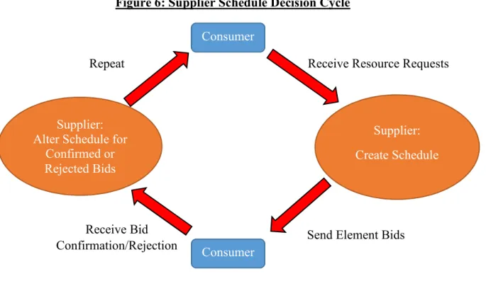
2.2.1 Incomplete Fulfillment
Element Bid outcome one is relatively straightforward to manage in an e-commerce network. For Incomplete Fulfillment, the consumer rebroadcasts the original task request. This request is made in the hopes that a previously busy supplier now has room in its schedule. Suppliers are constantly altering schedules through bidding rounds, as seen in Figure 6, as scheduled tasks receive bid rejections.
Yes
Task Created
Are bidding rounds over?
Task is abandoned
Resource Request sent to Suppliers
Bids received?
Complete Fulfillment
Incomplete Fulfillment Unsynchronized Fulfillment
No
Selected Bids are from one Supplier
Select cheapest Bids
Selected Bids are from multiple Suppliers
Secure Time Window* Send Bid Conf./Rej.
Execute Task
18
Figure 6: Supplier Schedule Decision Cycle
2.2.2 Complete Fulfillment
For element bid outcome two, Complete Fulfillment, the consumer will select which combination of bids they need at the cheapest cost. The consumer shall notify suppliers of unselected bids that their bid was rejected and should thus be dropped from that supplier’s schedule. As mentioned in the beginning of Chapter 2, consumers are assumed to be honest agents that do not hoard unnecessary resources. Consumers will only accept the bids they need to fulfill a task’s resource requirements. Should an allocated resource suddenly become
unavailable, a consumer can always re-submit a resource request in the next bidding round. Of note in the Consumer Decision Process, Figure 5, is the route of “Selected Bids are from one supplier.” When a single supplier is providing all the resources for a task, they have control over the tasks start and end time, as long as it remains within the original time window. Even if a consumer accepts a bid (or bids) for a specific start time, the supplier can change that start time as they see fit. If this previously agreed upon start time were made rigid, the supplier may drop this commitment in favor of a new more valuable task request. The supplier’s
flexibility to move start times, only if it is allocating all the resources needed, is advantageous to consumers as it lowers the risk of bids being withdrawn. This is also advantageous to the system
Receive Resource Requests
Supplier: Create Schedule
Send Element Bids Supplier:
Alter Schedule for Confirmed or Rejected Bids Consumer Consumer Receive Bid Confirmation/Rejection Repeat
19
as suppliers have flexibility in their schedule to open up slots for tasks that may be denied from schedules made in earlier bidding rounds.
When a consumer selects resources from multiple suppliers, the “Secure Time Window” stage is necessary. This simply alters the task to begin and end only at the time all element bids overlap. This is necessary as the original resource request specified a time window with a range of possible arrive and depart times for suppliers to offer resources in. Once a set of bids that completely fulfill the task are found, consumers do not want these resources’ time slots to be move around by suppliers, resulting in the task becoming unsynchronized. To prevent this, consumers secure the task’s time window to one start and end time that all element bids overlap. Suppliers are updated of this change to the task’s information through the bid confirmations sent. 2.2.3 Unsynchronized Fulfillment
Element bid outcome three, Unsynchronized Fulfillment, presents the greatest challenge for consumers. As suppliers are not communicating with each other, consumers rebroadcasting the same request leaves synchronization to chance. Progressing to complete fulfillment requires direction from the consumer to coordinate scheduling across suppliers.
This “Decide” phase of the OODA loop in the Consumer Decision Process attempts to balance task feasibility with synchronization. The wider the range of the time window for the task, the greater the likelihood a resource request will be answered as suppliers have many options to fit servicing the task into their schedule. The drawback of these numerous options for suppliers is the decreased probability Element Bids will then be synchronized with other
suppliers whose schedules are unknown. To push diverse suppliers towards coordination, a consumer updates the time window.
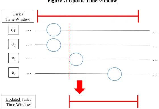
The time window is updated by pushing the task’s early time window to the second earliest bid arrival time. This heuristic is based on ICAARUS pushing all tasks to be serviced as early as feasible. This means that when a bid is received, the consumer knows the resource cannot be moved any earlier without altering the schedule. However, the resource could be moved back and the schedule remains feasible with idle time in the later part of the resource path. An example of updating the time window is shown in Figure 7:
20
Figure 7: Update Time Window
Updating to only the second earliest bid arrival time is crucial to synchronizing suppliers without forcing schedules to sub-optimal solutions. As can be seen in Figure 7, even with the new shortened time window, all four Element Bids are not synchronized. While suppliers may push bids e1 and e2 to have the same arrival time as e3, e4’s arrival time may not be moved up. In that case the task will again reach Unsynchronized Fulfillment status and the time window will be shortened to e4’s arrival time, and then the task is expected to reach synchronization across all Element Bids.
The task’s early time is not immediately updated to the latest arrival time, e4’s arrival time, as that may tighten the task’s time window to an infeasible time range. Suppose one supplier was providing bids e1 and e2, and it has a highly valuable task it is servicing right after task i that it cannot move. If the time window were drastically tightened then task i would lose two of its Element Bids. By gradually updating the time window through multiple bidding rounds, the following rounds could have the supplier of e4 move its arrival time up or new suppliers become able to service task i in place of e4’s supplier.
If the updating time window process results in a supplier dropping its Element Bid for the task with no other supplier filling its bid, then the task would become an Incomplete Fulfillment
… … … … … … … … Task i Time Window Updated Task i Time Window e1 e2 e3 e4
21
case. This would result in the consumer re-submitting its resource requests with the task’s original time window, giving maximum flexibility to suppliers again.
22
Chapter 3
3
Model Formulation and Development
This chapter develops a mathematical representation that addresses the Supplier Scheduling Problem (SSP). The mathematical representation begins with a description of the input and output variables that define the problem. The mathematical structure of the SSP is visualized through multiple graphical representations to highlight the network nature of this problem.
The mathematical formulation allows us to identify similar problems in the literature. Research into the Traveling Salesman Problem and its Time Window variants help us understand the challenges of SSP and provide techniques for finding solutions through exact and heuristic methods. The Team Orienteering Problem is also a useful variant of the Traveling Salesman Problem for understanding and current methods used for organizing a team to maximize prize collection as the SSP organizes multiple resources for maximum mission completion.
At the end of the chapter, a Mixed Integer Programming (MIP) model of the SSP is presented. This MIP utilizes binary and continuous decision variables to build a schedule for a set of resources that satisfies the constraints of the SSP.
Supplier Scheduling Problem (SSP)
This section describes the SSP and defines the inputs and outputs of the problem. It presents assumptions that were made on the capabilities of the resources, and explains any other assumptions made to simplify operational constraints for the purpose of this mathematical model.
3.1.1 Inputs to Supplier Solver 3.1.1.1 Supplier Inputs
supplierID Integer value identifying which supplier is making this schedule.
23
resourceList Set of-which resources and what quantity of those resources a
supplier has control over.
schedule Assignments of which task elements a supplier has committed
particular resources too, and what time they are assigned to service these requests.
unconfirmedTasks Set of which tasks the supplier has on its schedule that it bid to fulfill for a consumer, but has not received a status notification of yet.
confirmedTasks Set of which tasks the supplier has on its schedule that it has bid on and an acceptance of selection has been received by a consumer. The supplierID, pos, and resourceList are unchanging for each supplier through all rounds of bidding. Initially the schedule, unconfirmedTasks, and confirmedTasks are empty until the supplier begins bidding on task requests.
The resourceList can have duplicate entries to express a supplier’s capacity of multiple resources for that one type. For example: a resourceList of {A,B,C} means a supplier has one resource of type A, one resource of type B, and one resource of type C. Meanwhile a resourceList of {A,A,A} means a supplier has three resources of type A.
3.1.1.2 Task Inputs
consumerID Integer value identifying which consumer the task request is from.
taskID Integer value a consumer gives to identify the task.
pos Position of the task’s location.
value Rated importance of the task from [1-100].
early Beginning of time window for the task.
late End of time window for the task.
24
resourceCount Number of elements for which the task is requesting resources.
resourceReq Set of resources the task is requesting.
A task request has two forms of identification, consumerID & taskID. From here onward a task may be referred to as simply task i or task j, but this i or j is not a task’s complete ID, it is merely a shorthand to index individual tasks. For example: task i could be referring to task (2,3), which is a task from consumer 2 and labeled as task 3 from that consumer.
The resourceReq can have duplicate entries to express the consumer needing multiple resources of that one type for a task. For example: a resourceReq of {A,B,C} means a task is requesting three elements with one resource of type A, one resource of type B, and one resource of type C. Meanwhile a resourceReq of {A,A,C} means a task is requesting three elements with two resources of type A, and one resource of type C.
3.1.2 Outputs of Supplier Solver
As mentioned in the motivation for this research, the model is decentralized in nature for its bidding structure. So, the outputs from a supplier that a consumer would see are bids for task elements. However, the solution to the SSP is a schedule of supplier resources accommodating tasks, which remains visible only to that individual supplier. A supplier’s schedule is described as a list of composites:
composite A single resource and a path plan
The path of a composite has the following characteristics:
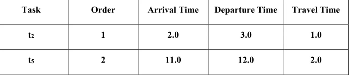
1. Task Order: The order in which this resource will accommodate its assigned tasks. 2. Arrival Times: The time at which the resource will be able to start each task assigned. 3. Departure Times: The time at which the resource will need to end each task assigned. 4. Travel Times: The time required to travel from the previous task to the subsequent task. Example 1 displays a supplier’s schedule with composites.
25
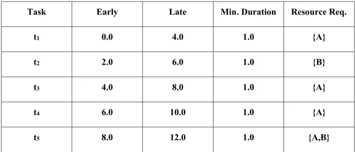
Example 1: This example describes a schedule with two composites, meaning two resources and two path plans. Here there is a set of five tasks, {t1,t2,t3,t4,t5}, to be completed by a set of two resources, {A,B}. The following is a table of a selection of the parameters for this set of tasks:
Table 1: Example 1 Task Parameters
Task Early Late Min. Duration Resource Req.
t1 0.0 4.0 1.0 {A}
t2 2.0 6.0 1.0 {B}
t3 4.0 8.0 1.0 {A}
t4 6.0 10.0 1.0 {A}
t5 8.0 12.0 1.0 {A,B}
Only task t5 requires multiple resources and needs synchronization across resources. The following provides path plans for the composite example:
Composite 1. Resource A departs the base station at time 0, and then performs the following tasks. The resource returns to the base station directly after completing t5:
Table 2: Example 1 Composite 1: Path Plan for Resource A
Task Order Arrival Time Departure Time Travel Time
t1 1 1.0 2.0 1.0
t3 2 4.0 5.0 1.0
t4 3 7.0 8.0 2.0
t5 4 11.0 12.0 3.0
Note that the while resource A can begin t1 at time 0, it takes a travel time of 1 hour to get to that task (from starting base) so its arrive time is 1.0. Also, while resource A can leave t1 at
26
time 2.0, and it only requires a travel time of 1 hour to get to t3 at time 3.0, the resource cannot begin servicing the task till t3’s Arrive Time of time 4.0.
Composite 2. Resource B only requires a travel time of 1 hour to get to t2 from the base station, so it does not depart till time 1.0, and then performs the following task. The resource returns to the base station directly after completing t5:
Table 3: Example 1 Composite 2: Path Plan for Resource B
Task Order Arrival Time Departure Time Travel Time
t2 1 2.0 3.0 1.0
t5 2 11.0 12.0 2.0
Note that while resource A can leave t2 at time 3.0, and it only requires a travel time of 2 hours to get to t5 at time 5.0, the resource does not begin servicing the task till time 11.0 even though the time window for servicing the task is time 8.0. This is because t5 requires
synchronization of both resources, so resource B must wait for resource A to arrive to begin servicing t5 together.
Network Representation
This section describes how to transform the physical real-world problem with complex parameters, into a graphical structure easier to visualize. This formulation of the problem into a graph will provide insight into methods to solve the problem. First introduced is a simplistic static graph of the problem, then a more complex time-space graph, and finally a placement-space graph.
3.2.1 Static Graph Representation
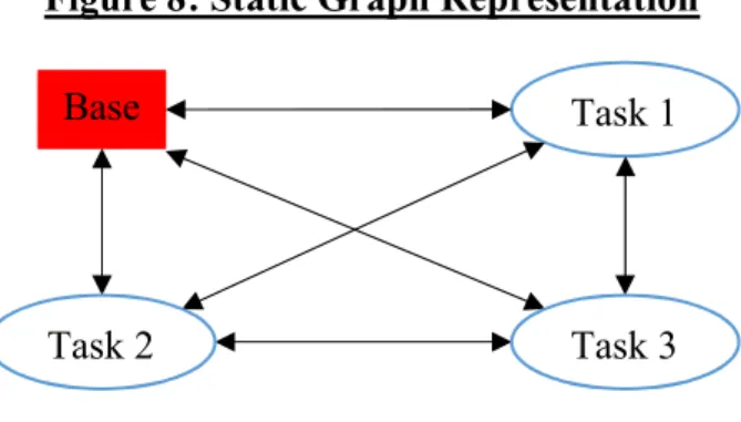
To begin applying analytical techniques to the SSP, the physical system should be mapped to the proper theoretical framework. Large-scale transportation problems, such as the Vehicle Routing Problem, are often represented using a directed graph, G(N,A), consisting of a set of nodes, N, and a set of arcs, A [15]. In this network the nodes represent task and base locations, and arcs represent the path to get from one node to another. A two-dimensional map
27
can be rearranged to a simpler network to visualize with weights on those arcs representing the distance between node pairs. A static graph representation for the operations of a single resource and three tasks is shown in Figure 8:
Figure 8: Static Graph Representation
3.2.2 Time-Space Graph Representation
The static graph representation presented in the previous section is unable to model the time dimension of resource scheduling. To model time and position, the time-space graphical representation can incorporate time by creating nodes that include the location of the resource and the time that the resource is at the task. Therefore, a node most be created for each task at every time period over the planning horizon. Task-time nodes cannot be limited to only be the time periods for which the task’s time window is active as the network needs to capture where the resource is if the resource is idly waiting between two time windows.
The time-space graph assists in scheduling resources, because it records the location of every resource at each point in time. Each node in the time-space graph is indexed by task and time period. For example, index (i,t) corresponds to task i at time t. However, now the arcs must become directed in the network as travelling back in time is prohibited in reality. below we show Figure 9 of a time-space graph with two tasks:
Task 1 Base
Task 3 Task 2
28
Figure 9: Time-Space Graph Representation
While this network enables visualizing a resources position in space and time, it creates many unnecessary nodes and arcs due to task nodes existing across the whole planning horizon. Another issue this graph representation encompasses is the need to discretize time. The drawback of high precision with shrinking time intervals comes at the cost of rapidly growing the number of nodes.
3.2.3 Placement-Space Graph Representation
The time-space graph representation in the previous section suffers in the trade-off of precision of time vs. graph size. When a continuous variable such as time is binned into discrete segments, the ease of interpretation comes at the risk of suboptimal solutions. To keep time of arrivals and departures as continuous variables, the placement-space graphical representation incorporates order by creating nodes that include the location of the resource and the placement that the resource is in the service list. This requires a node to be created for each task at every index on the resource’s service list. This is expected to create a graphical representation with fewer nodes as the number of tasks to accommodate should be significantly smaller than the number of time periods in the planning horizon.
Each node in the placement-space graph is indexed by task and placement. For example, index (i,2) corresponds to task i being the second task the resource visits. The arcs must also be directed as the time-space graph, as traveling back in order is prohibited in reality. Below we show Figure 10 of a placement-space graph with two tasks:
Base,t
i,t+1 i,t+2
j,t+2 j,t+1
Base,t+1 Base,t+2 Base,t+3
i,t+2
29
Figure 10: Placement-Space Graph Representation
A path through this network reveals which tasks the resource will be able to service and in what order the tasks will be accommodated. However, like the time-space graph, the time window and synchronization constraints are not implicitly expressed and will require additional constraints on the network’s arcs. The placement-space graph does require less arcs and nodes than the time-space graph, while maintaining continuous time variables.
Problem Classification
Now that the parameters of the problem are defined and a visual representation can be created for the placement-space dimension of the problem, similar problems in literature are compared to lend more insight to solution formation. The Vehicle Routing Problem (VRP) has many similarities to a supplier attempting to find an optimal routing of its resources. After all a vehicle is just a specific type of resource. The VRP has been studied since 1959’s work by Dantzig and Ramser, and so many variations and formulations exist to draw inspiration from [16]. This section aims to classify previous research methods similar to the SSP’s goals of maximizing benefit received while handling elements of:
Time
Multi-resource Synchronization Resource classes
In addition to accomplishing these features, there is also the desired feature of quickly finding a solution for a large number of tasks.
Base,0
i,1 i,2
j,2 j,1
30 3.3.1 Mathematical Programming Background
A proven field of research for solving the VRP is known as Linear Programming. Linear Programming makes use of abstract mathematical models to represent real-world problems. The name “linear” comes from the linear functions of the decision variables that form the objective and all constraints. By formulating the rewards and costs of a real-world problem into an objective function, linear programming can find an exact solution that maximizes or minimizes this value. It does this under a set of constraints that represent the real-world conditions that limit the problem [12].
The classical linear programming problem necessitates all variables are continuous non-negative real numbers. This is not the case for a problem such as resource scheduling that requires binary decision variables, and a “yes” or “no” answer to the question of allocation. This is because a resource, such as a vehicle, cannot be cut in half and used to service half of two requests. A resource must be sent in its integral entirety or not at all. Fortunately, this a well-studied problem in the realm of Mixed Integer Programming (MIP), which is classified as a subset of mathematical programming using integer and binary variables. The unique types of problems faced in the SSP also fall under a more general class of problems known as the Traveling Salesman Problem (TSP) [17].
3.3.2 Travelling Salesman Problem
Dantzig describes the Traveling Salesman Problem as “Find the shortest route for a salesman starting from a given city, visiting each of a specified group of cities, and then returning to the original point of departure” [18]. It is a mathematical conjecture that the complexity class of the TSP is Nondeterministic Polynomial-time Complete or NP-Complete [19]. This means that there is no known algorithm that can always give an optimal solution in a polynomial time variation. The best that can be done currently is finding a solution to an NP-Complete problem that has solution times grow exponentially with the number of nodes [20]. 3.3.2.1 Mixed Integer Programming Formulation for Traveling Salesman Problem
The TSP can be modeled as a MIP with binary variables that indicate the decision whether or not to traverse an arc in the network. The variable, xij, will take on the value of one if the arc
31
between node i and node j is traveled, and zero otherwise. The variable, dij, is the distance from node i to node j. Dantzig, Fulkerson, and Johnson give the following MIP model:
𝑀𝑖𝑛𝑖𝑚𝑖𝑧𝑒 ∑( , )∈ 𝑑, 𝑥,
𝑆𝑢𝑏𝑗𝑒𝑐𝑡 𝑡𝑜: ∑∈ 𝑥, = 2 ∀𝑗 ∈ 𝑁
∑, ∈ 𝑥, ≤ |𝑆| − 1 ∀𝑆 ⊂ 𝑁, 𝑆 ≠ ∅
𝑥, ∈ {0,1}
The set N is the set of all nodes in the network, and S is a subset of N. The first constraint ensures that each node in the network is visited by forcing the traveler to travel into and out of each node. The second constraint is a sub-tour elimination constraint; it ensures that the solution is a single tour. The size of the problem increases exponentially with the addition of the sub-tour elimination constraint, adding 2N constraints.
3.3.2.2 Exact Solution Methods
All known solution methods to TSP run in non-polynomial time, and in the worst case the entire solution space might have to be searched to confirm an optimal solution. However, there are methods that attempt to intelligently search the solution space and reduce the solve time for the model. Two of the most common methods are branch and bound and cutting planes.
The branch and bound method is a divide and conquer method to find an optimal solution. This method begins by solving the linear programming relaxation, which removes the constraints that ensure variables are integral and binary [19]. This means the xij variable can take on continuous values between zero and one and will provide a “lower bound” to the solution that may or may not be attainable. Next, this method solves sub-problems in an attempt to find integer solutions. The lower bound is used to discard certain subsets of the feasible set from consideration [20].
The cutting planes method begins similarly to branch and bound by first solving the linear programming relaxation. Next, sub-tour elimination constraints are added to force fractional solutions towards integer solutions, as well as to get rid of any sub-tours in the
32
relaxation solution [18]. In the right circumstances, only a few intelligently chosen constraints are needed to find an optimal solution to all constraints.
3.3.2.3 Heuristic Solution Methods
When an exact solution method is relaxed to only need near-optimal solutions, but in a shorter search time, heuristic solution methods can be used to generate quick solutions.
Heuristics do not search the entire set of solutions, but find the “best” solution in a reasonable amount of time. “Best” is defined as a threshold the designer creates for the acceptable gap from optimality.
Laporte categorizes heuristic methods into two classes: 1. Tour construction procedures to efficiently build feasible routes by adding nodes one at a time, and 2. Tour improvement procedures to improve an already existing route [21]. Most heuristic algorithms that solve the TSP incorporates both tour construction and tour improvement procedures in what is called a composite algorithm [21]. Note here the name “composite” refers to the algorithm being a combination of multiple procedures, and is not an algorithm of composites as defined in Section 3.1.2.
For example, Flood suggests the nearest neighbor algorithm is a straightforward tour construction procedure to find a solution to the TSP [22]. This algorithm begins at an arbitrary node, and proceeds to add the node that is closest to the present node. It repeats this nearest neighbor addition to the route until all nodes are included in the path. The last node is then connected to the origin to create a complete tour.
Another class of tour construction procedures, known as insertion algorithms, follow these basic steps [21]:
Step 1: Construct a simple tour with only two nodes
Step 2: Consider each node not in the tour. Insert the node that meets a specific criterion. Common criteria that are used to measure which node is most appropriate to be added next to the network include: 1. Adding the node that is closest to the two nodes in the current selected tour, 2. Adding the node that is furthest from the two nodes in the current selected tour, and 3. Adding the node that produces the least increase in distance for the current path. While
33
these examples of criteria are not exhaustive, other criteria include combining multiple metrics with weights assigned to each method [23].
Tour improvement procedures already start with a route, built by a simple or complex construction procedure. These procedures then aim to improve this given route by some routine. Flood noticed that if a path crosses itself at any point during the tour, then the tour could be improved by switching the order of nodes so that the tour does not cross [22]. Croes proposed a similar idea, known as inversion¸ where the order of two nodes is switched in a tour to see if the resulting route is improved [24]. Lin and Kernigan expanded upon these methods to bound the scope of searching for tour improvements in the k-opt algorithm [25]. The algorithm goes through all subsets of k arcs and attempts to reconnect the tour with a set of k new arcs. If an improvement is found, the k old arcs are deleted in favor of the new better arcs, and the
algorithm continues down the route to the next set. An example of a k-opt algorithm with k = 2 is shown in Figure 11:
Figure 11: 2-Opt Algorithm
Another group of tour improvement procedures are metaheuristics. These methods include subroutines that select which scope of the solution set to explore. These heuristics
Original Route: [1,2,5,3,4] 1 2 3 4 5 1. Arc (2,5) replaced with (2,3) 2. Arc (3,4) replaced with (5,4) Improved Route: [1,2,3,5,4] 1 2 3 4 5
34
include tabu search, which records which solutions have already been generated to avoid repeated searches, ant colony, which records which previous solutions led to improvements and should be explored more, and simulated annealing, selecting solutions with a probability based on a measured criterion of optimality [26]. Simulated annealing is used extensively in
ICAARUS as detailed in Chapter 4.
3.3.3 Traveling Salesman Problem with Time Windows
The TSP with Time Windows (TSPTW) is very similar to the basic TSP with extra constraints on when the salesman can visit a city. Each city has a time window in which the salesman can visit the city. Arriving in the city before or after that time window does not count as a visit for the salesman. The objective remains to visit N nodes at least once (within their time windows) at a minimum travel cost.
In linear programming these time windows would be expressed as a constraint the Salesman must visit the city after the time window’s lower bound, li, and before the time
window’s upper bound, ui. Baker proposed a model with decision variables, ti, that specified the time the Salesman visited city i. The shortest travel times between each node pair is already found and expressed by dij .The decision variable tn+1 specifies the time the salesman returns to the start node, and it is the difference between this time and the start time, t0, that is trying to be minimized [28]. 𝑀𝑖𝑛𝑖𝑚𝑖𝑧𝑒 𝑡 − 𝑡 𝑆𝑢𝑏𝑗𝑒𝑐𝑡 𝑡𝑜: 𝑡 − 𝑡 ≥ 𝑑 𝑖 = 2, … , 𝑛 |𝑡 − 𝑡 | ≥ 𝑑 𝑖 = 3, … , 𝑛 2 ≤ 𝑗 ≤ 𝑖 𝑡 − 𝑡 ≥ 𝑑 𝑖 = 2, … , 𝑛 𝑡 ≥ 0 𝑖 = 1, … , 𝑛 + 1 𝑙 ≤ 𝑡 ≤ 𝑢 𝑖 = 2, … , 𝑛
In scenarios with many cities for the salesman to visit, a large |N|, this solution scales poorly and can take a long time to solve. Another exact algorithm to solve the TSPTW was
35
introduced by Mingozzi et al. through use of precedence constraints [27]. Precedence constraints in a route ensure a node is visited no earlier than the proceeding node is visited. These
constraints ensure that in tour construction, the next node added in the route is always in time order. A faster, but inexact, approach was proposed by Gendreau et al. that utilizes the nearest neighbor algorithm to construct tours [29]. This method requires at each iteration, that the time window bounds be checked for the added city to ensure the solution constructed is feasible. 3.3.4 Team Orienteering Problem
The Orienteering Problem (OP), or generalized TSP, is described as: given n nodes, each node i has a non-zero score 𝑠 . The arc between node i and j has an associated cost of cij. In this problem the travel time between each node represents the cost and each node can be visited at most once. The objective of the OP is to maximize the score of a path that consists of a subset of nodes beginning at node 1 and ending at node n without violating the max cost (travel time) constraint T.
Golden et al. demonstrate this model for the sport of orienteering has useful application to the VRP and production scheduling [30]. They also proved that the OP is NP-hard, warning of the computational limitations of exact methods and encouraging a focus on heuristic procedures for problems of these classification. Golden et al. present a composite algorithm where the first stage constructs routes through a cost-benefit analysis and the second stage improves the initial route by 2-opt method similar to Lin-Kernigan and then a center-of-gravity method. Golden, Wang and Liu produced a more efficient algorithm where the algorithm learns the most effective route improvement methods and adapts through the course of improvements [34]. Tsiligrides approached the OP with a two stage heuristic, building initial routes through a Monte Carlo approach, and improving routes through a local search space heuristic method that performs route optimization similar to Lin-Kernigan’s 2-opt method [33]. Ramesh and Brown solve the OP by iterating through four phases [35]:
1. Construct an initial route by a cost-to-benefit analysis to see which node is best to add next on the route.
36
3. Select nodes to delete from route that can be replaced with more valuable nodes in their places.
4. Repeat until the marginal improvement of a round falls below a specified threshold. The Team Orienteering Problem (TOP) extends the OP by creating multiple tours of the network for multiple Orienteers to maximize the score collected. In the sport or orienteering a team of Orienteers attempt to coordinate together to collect as many waypoints as possible in a given amount of time. This aspect of coordination adds a great deal of complexity to the problem. Tang and Miller-Hooks used the heuristic of tabu search to overcome these complexities in TOP [31]. Following their work, Archetti et al. compared tabu search with variable neighborhood search and found that Variable Neighborhood Search outperformed two tabu search heuristics [32]. Adaptive Large Neighborhood Search, an extension of Variable Neighborhood Search, is explored further in Chapter 4 as a solution to the SSP.
Mixed Integer Linear Programming Model
This section discusses a Mixed-Integer Linear Programming (MILP) formulation that can be readily formatted to optimization software. The mathematical model provides the ability to find an exact optimal solution. Although previous research has shown that exact methods might not be practical, the optimal solution will give insight to compare the quality of a solution generated through heuristic methods. In addition, the linear programming relaxation of this model, while inexact, will give a quick theoretical upper limit to the “best solution.” This upper limit can be useful to evaluate the gap between LP and heuristic methods in a time efficient manner.
This work draws heavily from Miller’s reformulation of the Team Orienteering Problem with Time Windows (TOPTW) to solve his Unmanned Surface Vessel Observation-Planning Problem (USVOPP) [12]. The MILP developed by Miller took advantage of integer decision variables to create of placement-space nodes in network which greatly inspired this particular model. Miller’s binary variable 𝑥 takes a value of 1 if node i is visited by USV k in the t-th placement on the route, encompassing multiple decisions in a single variable. Also instrumental to the development of this model was Negron’s work in creating a MILP model to make
37
travel time constraints by introducing linearization variables that are calculated a priori, which is key to formulating this particular model [7].
3.4.1 Supplier MILP Model Formulation
This mathematical formulation is used by individual suppliers to find the optimal schedule for a supplier’s resources for all the task requests received. First the notations for sets, decision variables, and input variables are defined. Then the objective function and constraints are introduced. Finally variations of this model are introduced to improve synchronization of element bids for a particular task.
3.4.1.1 Set Definitions
The following sets are used in the formulation: T = set of all tasks
U = set of all resources
U(e) = Set of all resources of type e P = set of all placements in a path
The set P is the set of placements of tasks in a path for a resource. A placement denotes the order of a task in the path. For example, if a task is in placement three, then the task is the third task that will be performed by the resource. The set of placements contain the placement for each task in the path. For Example: The set associated with a path of five tasks, T={t1,t2,t3,t4,t5}, will contain the first five natural numbers, P={1,2,3,4,5}.
3.4.1.2 Decision Variables
accommodatei,u,p A binary decision variable of 1 if task i is accommodated by resource u in placement p, 0 otherwise.
traveli,j,u A binary decision variable of 1 if the arc from task i to task j is travelled by resource u, 0 otherwise.
arrivei,u A continuous decision variable that assigns the time that resource u
38
departi,u A continuous decision variable that assigns the time that resource u
will depart from task i.
Note where Negron and Miller make use of a decision variable named perform, this work uses the decision variable accommodate. This is to reflect that even though a resource of a supplier may be assigned to a specific task, it is not guaranteed to perform that task by the consumer, thus it has only been allocated to “accommodate” a task at this stage.
3.4.1.3 Input Variables
earlyi Beginning of time window for task i.
latei End of time window for task i.
minDuri Required time to complete task i.
horizon Planning horizon.
travelTimei,j,u Length of time for resource u to travel from location of task i to location of task j.
travelToBaseTimei,u Length of time for resource u to travel from location of task i to location of u’s supplier.
resourceCounti,e The number of elements that task i requests for a resource type e.
valuei The value to complete task i.
3.4.1.4 Objective Function
The objective is to maximize the total value of all tasks completed. Each task has a varying number of resources request, some tasks may only request one resource, and others may request multiple resources. Thus, the value of a task is divided by the number of resources requested so that the full value can only be achieved if all the resources requested are accommodated. The objective function is:
39 3.4.1.5 Constraints
The model has twelve constraints that are categorized as resource type constraints, network constraints, or time window constraints. The constraints ensure that the capacities of suppliers and capabilities of resources are not exceeded, so that the resulting schedule for resources is feasible for all suppliers to fulfil. The resource type constraints ensure that a resource of one type does not accommodate a task element request of a different type. The following is the resource type constraints:
(1) Ensure a Task, i, cannot be accommodated by a resource, u, it does not request.
𝑎𝑐𝑐𝑜𝑚𝑜𝑑𝑎𝑡𝑒, , = 0 ∀𝑖 ∈ 𝑇, 𝑒 ∈ 𝑖, 𝑢 ∉ 𝑈(𝑒), 𝑝 ∈ 𝑃
The network constraints ensure that the resulting operations scheduling creates a feasible path for the resources’ schedule. The following are the network constraints:
(2) Each Task, i, can only be assigned one placement per resource.
∑ ∈ 𝑎𝑐𝑐𝑜𝑚𝑜𝑑𝑎𝑡𝑒, , ≤ 1 ∀𝑖 ∈ 𝑇, 𝑢 ∈ 𝑈
(3) Each placement, p, can only be assigned one task per resource.
∑∈ 𝑎𝑐𝑐𝑜𝑚𝑜𝑑𝑎𝑡𝑒 , , ≤ 1 ∀𝑢 ∈ 𝑈, 𝑝 ∈ 𝑃
(4) Ensure each Task, i, does not get more resources, u, per element type of its request. ∑ ∈ ( )∑ ∈ 𝑎𝑐𝑐𝑜𝑚𝑜𝑑𝑎𝑡𝑒, , ≤ 𝑟𝑒𝑠𝑜𝑢𝑟𝑐𝑒𝐶𝑜𝑢𝑛𝑡, ∀𝑖 ∈ 𝑇, 𝑒 ∈ 𝑖 (5) Ensure that the tasks are assigned in successive placements on the resource path.
∑∈ 𝑎𝑐𝑐𝑜𝑚𝑜𝑑𝑎𝑡𝑒, , − ∑∈ 𝑎𝑐𝑐𝑜𝑚𝑜𝑑𝑎𝑡𝑒, , ≤ 0 ∀𝑢 ∈ 𝑈, 𝑝 ∈ 𝑃 − 1
(6) Force a travel arc to exist between two tasks performed successively.
𝑎𝑐𝑐𝑜𝑚𝑜𝑑𝑎𝑡𝑒 , , + 𝑎𝑐𝑐𝑜𝑚𝑜𝑑𝑎𝑡𝑒, , − 2 ∗ 𝑡𝑟𝑎𝑣𝑒𝑙, , ≤ 1 ∀𝑖 ∈ 𝑇, 𝑗 ∈ 𝑇,
∀𝑢 ∈ 𝑈, 𝑝 ∈ 𝑃 − 1
The time window constraints limit the resulting operations scheduling to performing tasks within the desired time window. The following are the time window constraints:
40
(7) Resource must arrive after the beginning of the time window if it is accommodating task i.
𝑒𝑎𝑟𝑙𝑦 × ∑ ∈ 𝑎𝑐𝑐𝑜𝑚𝑜𝑑𝑎𝑡𝑒, , ≤ 𝑎𝑟𝑟𝑖𝑣𝑒, ∀𝑖 ∈ 𝑇, 𝑢 ∈ 𝑈
(8) Resource must exit before end of time window if it is accommodating task i.
ℎ𝑜𝑟𝑖𝑧𝑜𝑛 − (ℎ𝑜𝑟𝑖𝑧𝑜𝑛 − 𝑙𝑎𝑡𝑒 ) × ∑ ∈ 𝑎𝑐𝑐𝑜𝑚𝑜𝑑𝑎𝑡𝑒, , ≥ 𝑑𝑒𝑝𝑎𝑟𝑡,
∀𝑖 ∈ 𝑇, 𝑢 ∈ 𝑈
(9) Resource can depart the task only after the minimum required duration of time.
𝑎𝑟𝑟𝑖𝑣𝑒, − 𝑚𝑖𝑛𝐷𝑢𝑟 × ∑ ∈ 𝑎𝑐𝑐𝑜𝑚𝑜𝑑𝑎𝑡𝑒, , ≤ 𝑑𝑒𝑝𝑎𝑟𝑡, ∀𝑖 ∈ 𝑇, 𝑢 ∈ 𝑈
(10) Resource must begin schedule at location of supplier’s base.
𝑡𝑟𝑎𝑣𝑒𝑙𝑇𝑜𝐵𝑎𝑠𝑒𝑇𝑖𝑚𝑒, ≤ 𝑎𝑟𝑟𝑖𝑣𝑒, ∀𝑖 ∈ 𝑇, 𝑢 ∈ 𝑈
(11) Resource must end schedule at location of supplier’s base.
𝑑𝑒𝑝𝑎𝑟𝑡, ≤ ℎ𝑜𝑟𝑖𝑧𝑜𝑛 − 𝑡𝑟𝑎𝑣𝑒𝑙𝑇𝑜𝐵𝑎𝑠𝑒𝑇𝑖𝑚𝑒, ∀𝑖 ∈ 𝑇, 𝑢 ∈ 𝑈
(12) Ensure sufficient travel time between tasks. 𝑎, , must be calculated a priori as explained in Subsection 3.4.1.6
𝑑𝑒𝑝𝑎𝑟𝑡, + 𝑡𝑟𝑎𝑣𝑒𝑙𝑇𝑖𝑚𝑒, , − 𝑎 , , (1 − 𝑡𝑟𝑎𝑣𝑒𝑙, , ) ≤ 𝑎𝑟𝑟𝑖𝑣𝑒,
∀𝑖 ∈ 𝑇, 𝑗 ∈ 𝑇, 𝑢 ∈ 𝑈
3.4.1.6 Linearization of Constraint
The LP model needs to constrain the time that a resource arrives at a subsequent task to be greater than the time that it takes to arrive at that following task, which is the time it departs the previous task plus the travel time between the two tasks. The intuitive way to write this constraint would be:
41
However, this constraint in not linear, because decision variables are being multiplied together. Therefore Ropke, Cordeau, and Laporte developed the following way to linearize the constraint ensuring sufficient travel time between two tasks [14]. The value, 𝑎, , , which must be calculated before solving the model, is:
𝑎, , = max 0, 𝑙𝑎𝑡𝑒 + 𝑚𝑖𝑛𝐷𝑢𝑟 + 𝑡𝑟𝑎𝑣𝑒𝑙𝑇𝑖𝑚𝑒, , − 𝑒𝑎𝑟𝑙𝑦
This constraint, (12), will now either be redundant with the non-negativity constraints (if the resource does not travel between the two tasks) or will constrain the departure time of the last task plus travel time to be less than the arrival time to the next task.
(12)= 𝑑𝑒𝑝𝑎𝑟𝑡 , − 𝑙𝑎𝑡𝑒, + 𝑚𝑖𝑛𝐷𝑢𝑟 ≤ 𝑎𝑟𝑟𝑖𝑣𝑒, − 𝑒𝑎𝑟𝑙𝑦, , 𝑡𝑟𝑎𝑣𝑒𝑙, , = 0
𝑑𝑒𝑝𝑎𝑟𝑡, + 𝑡𝑟𝑎𝑣𝑒𝑙𝑇𝑖𝑚𝑒, , ≤ 𝑎𝑟𝑟𝑖𝑣𝑒, , 𝑡𝑟𝑎𝑣𝑒𝑙, , = 1
3.4.2 Maximum Time Window Model Formulation
This e-commerce structure relies on two decision stages in each round of bidding, 1. the supplier deciding which tasks to service with which resources and when to service them and 2. the consumer deciding which resource bids have time windows overlapping that the consumer can accept to synchronize all the elements of a task. In stage 1, the supplier is trying to maximize the number of task elements accommodated which can result in very tight arrive and depart time windows.
As the supplier is trying to pack as many tasks into its sortie as possible to maximize the objective function, resources’ time windows usually only last for the required minimum duration even if they had idle time between that task and its following task. This becomes a problem in stage 2 when a consumer may have received bids for all its task elements, but they are all in different sections of the task’s initial time window. While these resources may be surrounded by idle time in which they could have stayed on the task longer and still had enough time to travel to their next task, this is not reported in the current MILP model. To address this inefficiency the concept of Maximum Time Window (MTW) is added to the model to increase the likelihood of task elements bids overlapping for consumer synchronization.
42 3.4.2.1 MTW Objective Function
The new objective function is very similar to the original model’s objective function of maximizing the total value of tasks completed, but it also aims to maximize the time window that the resource schedules for a task. The MTW objective function is:
𝑀𝑎𝑥 𝑣𝑎𝑙𝑢𝑒 𝑟𝑒𝑠𝑜𝑢𝑟𝑐𝑒𝐶𝑜𝑢𝑛𝑡 𝑎𝑐𝑐𝑜𝑚𝑚𝑜𝑑𝑎𝑡𝑒, , ∈ , ∈ ∈ + 𝑤 (𝑑𝑒𝑝𝑎𝑟𝑡, − 𝑎𝑟𝑟𝑖𝑣𝑒, ) ∈ , ∈
This objective function maximizes the time windows for bids by maximizing the
difference between the depart and arrive time for a resource to a task. An important parameter is
the weight for stretching the time windows, 𝑤 , as it controls the relationship of how
valuable accommodating a task is to maximizing the time window for accommodated tasks. Reminder: accommodate is a binary decision variable so can be {0,1}, while depart and arrive are continuous decision variables that are constrained by [0,latei - earlyi] (which for the context of this thesis is [0,25]).
In the most aggressive case for a supplier filling its sorties with as many tasks as possible, it will want to always choose to accommodate a task rather than maximize the time window of another task. For the particular parameters of this thesis, the weight should be set to:
𝑤 = 𝑎𝑐𝑐𝑜𝑚𝑚𝑜𝑑𝑎𝑡𝑒
𝑣𝑎𝑙𝑢𝑒 × ∆𝑡𝑖𝑚𝑒 𝑤𝑖𝑛𝑑𝑜𝑤 =
1
100 × 25= 0.0004
In more conservative cases where a supplier may want to allocate larger time windows
for high value tasks at the expense of not accommodating low value tasks, 𝑤 can be
increased depending on the desired ratio of large time windows to number of tasks accommodated.
3.4.2.2 Maximum Time Window Constraints
A constraint will need to be added to the original model as well to control the difference in depart and arrive times for non-accommodated tasks. Constraints (7) and (8) only restrict arrivei,u and departi,u when ∑ ∈ 𝑎𝑐𝑐𝑜𝑚𝑜𝑑𝑎𝑡𝑒, , = 1, so when inactive the difference in depart