DeepStance at SemEval-2016 Task 6: Detecting Stance
in Tweets Using Character and Word-Level CNNs
The MIT Faculty has made this article openly available.
Please share
how this access benefits you. Your story matters.
Citation
Vijayaraghavan, Prashanth, Ivan Sysoev, Soroush Vosoughi, and
Deb Roy. "DeepStance at SemEval-2016 Task 6: Detecting Stance
in Tweets Using Character and Word-Level CNNs." Proceedings
of the 10th International Workshop on Semantic Evaluation
(SemEval-2016), June 16-17, 2016, San Diego, California, ACL,
pp.413-419.
As Published
http://aclweb.org/anthology/S/S16/S16-1067.pdf
Publisher
Association for Computational Linguistics
Version
Author's final manuscript
Citable link
http://hdl.handle.net/1721.1/104351
Terms of Use
Creative Commons Attribution-Noncommercial-Share Alike
DeepStance at SemEval-2016 Task 6: Detecting Stance in Tweets Using
Character and Word-Level CNNs
Prashanth Vijayaraghavan, Ivan Sysoev, Soroush Vosoughi and Deb Roy MIT Media Lab, Massachusetts Institute of Technology
Cambridge, MA 02139
pralav@mit.edu, isysoev@mit.edu, soroush@mit.edu, dkroy@media.mit.edu
Abstract
This paper describes our approach for the De-tecting Stance in Tweetstask (SemEval-2016 Task 6). We utilized recent advances in short text categorization using deep learning to cre-ate word-level and character-level models. The choice between word-level and character-level models in each particular case was in-formed through validation performance. Our final system is a combination of classifiers us-ing word-level or character-level models. We also employed novel data augmentation tech-niques to expand and diversify our training dataset, thus making our system more robust. Our system achieved a macro-average preci-sion, recall and F1-scores of 0.67, 0.61 and 0.635 respectively.
1 Introduction
Stance detection is the task of automatically deter-mining whether the authors of a text are against or in favour of a given target. For instance, take the fol-lowing sentence: ”It has been such a cold April, so much for global warming.” This sentence’s author is most likely against the concept of global warm-ing (i.e., does not believe in it). The work presented here is specifically targeted towards detecting stance in tweets. The noisy and idiosyncratic nature of tweets make this a particularly hard task.
Automatic identification of stance in tweets has practical applications for a range of domains. For instance, it can be used as a sensor to measure the attitude of Twitter users on various issues, such as: political issues, candidates, brand names, TV shows, etc.
There has been extensive research done on mod-elling and automatic detection of stance in politi-cal arenas (e.g., debates) (Thomas et al., 2006) and on online forums (Somasundaran and Wiebe, 2009; Murakami and Raymond, 2010). However, as we alluded to earlier, the peculiar nature of tweets make techniques that have been developed for other plat-forms unsuitable. The field closest to this work is the field of Twitter sentiment classification, where the task is to detect the sentiment of a given tweet, usually as positive, negative, or neutral. Nonethe-less, it is important to note that there are substan-tial differences between sentiment classification and stance detection. Sentiment classifiers determine the polarity of a given tweet, without considering any targets (see Vosoughi et al. (Vosoughi et al., 2015) for an example of a Twitter sentiment classi-fier). For instance, consider the tweet: ”I love Don-ald Trump”, this tweet has a positive sentiment, and the author of the tweet has a positive stance towards Donald Trump, but it can also be inferred that the author is most likely against or at best neutral to-wards Bernie Sanders. In this paper, we present a system for automatic detection of stance in Tweets.
2 Our Approach
We trained a different model for each of the five tar-gets. Models for some of the targets used character-level convolutional neural networks(CNN), while other used word-level models. In one particular tar-get (Hillary Clinton), a combination of character-level and word-character-level models was used. Though Character-level models are robust to the idiosyn-cratic and noisy nature of tweets, they require a larger dataset compared to word-level models. Our
choice between the models was informed by valida-tion performance (as explained in secvalida-tion 5). The character and word-level models are explained in the section below.
2.1 Character-Level CNN Tweet Model
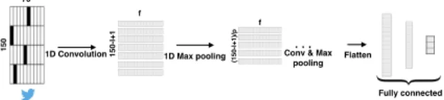
Character-level CNN (CharCNN) is a slight vari-ant of the deep character level convolutional neu-ral network introduced by Zhang et al (Zhang and LeCun, 2015), based on the success of CNNs in im-age recognition tasks (Girshick et al., 2014) (Hinton et al., 2012). In this model, we perform temporal (one-dimensional) convolutional and max-pooling operations. Given a discrete input function f (x) ∈ [1, l] 7→ R, a discrete kernel function k(x) ∈ [1, m] 7→ R and stride s, the convolution g(y) ∈ [1, (l − m + 1)/s] 7→ R between k(x) and f (x) and pooling operation h(y) ∈ [1, (l − m + 1)/s] 7→ R of f (x) is calculated as: g(y) = m X x=1 k(x) · f (y · s − x + c) (1) h(y) = maxmx=1f (y · s − x + c) (2) where c = m − s + 1 is an offset constant. In our implementation of the model, the stride s is set to 1. This model is illustrated in Figure 1. We adapted this model for the size limit of tweets (140 charac-ters). The character set includes English alphabets, numbers, special characters and unknown character. There are 70 characters in total, given below:
abcdefghijklmnopqrstuvw xyz0123456789-,;.!?:’"/ \| #$%&ˆ*˜‘+-=<>()[]{}
Each character in the tweet can be encoded using one-hot vector xi ∈ {0, 1}70. Hence, a tweet is
rep-resented as a binary matrix x1..150 ∈ {0, 1}150x70
with padding wherever necessary, where 150 is the maximum number of characters in a tweet plus padding and 70 is the size of the character set. Each tweet, in the form of a matrix, is now fed into a deep model consisting of four 1-d convolutional layers. A convolution operation employs a filter w, to extract l-gram character feature from a sliding window of l characters at the first layer and learns abstract tex-tual features in the subsequent layers. This filter
150 70 1 5 0 -l +1 f (1 5 0 -l +1 )/ p f
1D Convolution 1D Max pooling Conv & Max
pooling
…
Fully connected Flatten
Figure 1: Illustration of CharCNN Model
w is applied across all possible windows of size l to produce a feature map. A sufficient number (f ) of such filters are used to model the rich structures in the composition of characters. Generally, with tweet s, each element c(h,F )i (s) of a feature map F at the layer h is generated by:
c(h,F )i (s) = g(w(h,F ) ˆc(h−1)i (s) + b(h,F )) (3)
where w(h,F ) is the filter associated with feature map F at layer h; ˆc(h−1)i denotes the segment of out-put of layer h−1 for convolution at location i (where ˆ
c(0)i = xi...i+l−1 — one-hot vectors of l characters
from tweet s); b(h,F )is the bias associated with that filter at layer h; g is a rectified linear unit and is element-wise multiplication. The output of the con-volutional layer ch(s) is a matrix, the columns of which are feature maps c(h,Fk)(s)|k ∈ 1..f .
The output of the convolutional layer is followed by a 1-d max-overtime pooling operation (Collobert et al., 2011) over the feature map and selects the maximum value as the prominent feature from the current filter. Pooling size may vary at each layer (given by p(h) at layer h). The pooling operation shrinks the size of the feature representation and fil-ters out trivial features like unnecessary combina-tion of characters (in the initial layer). The window length l, number of filters f , pooling size p at each layer can vary for each classification task.
The output from the last convolutional layer is flattened and passed into a series of fully connected layers. The output of the final fully connected layer (sigmoid or softmax) gives a probability distribution over categories in our classification task. For regu-larization we apply a dropout (Hinton et al., 2012) mechanism after the first fully connected layer. This prevents co-adaptation of hidden units by randomly setting a proportion ρ of the hidden units to zero (Generally, we set ρ = 0.5). CharCNN can be ro-bust to misspellings and noise, provided there is suf-ficiently large dataset to train the model.
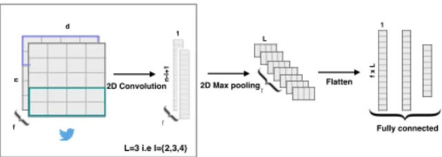
n -l +1 1 n d 2D Convolution f f f 2D Max pooling f x L 1 L=3 i.e l={2,3,4} L Fully connected Flatten
Figure 2: Illustration of Word-Embedding Convolutional Model
2.2 Convolutional Word-Embedding Model The convolutional embedding model (see Figure 2) assigns a d dimensional vector to each of the n words of an input tweet resulting in a matrix of size n × d. Each of these vectors are initialized with uni-formly distributed random numbers i.e. xi ∈ Rd.
The model, though randomly initialized, will even-tually learn a look-up matrix R|V |×d where |V | is the vocabulary size, which represents the word em-bedding for the words in the vocabulary.
A convolution layer is then applied to the n × d input tweet matrix, which takes into consideration all the successive windows of size l, sliding over the entire tweet. A filter w ∈ Rh×d operates on the tweet to give a feature map c ∈ Rn−l+1. We apply a max-pooling function (Collobert et al., 2011) of size p = (n − l + 1) shrinking the size of the resultant matrix by p. In this model, we do not have several hierarchical convolutional layers - instead we apply convolution and max-pooling operations with f fil-ters on the input tweet matrix for different window sizes (l).
The vector representations derived from various window sizes can be interpreted as prominent n-gram word features for the tweets. These features are concatenated to give a vector of size f × L, where L is the number of different l values which is further compressed to a size k before passing it to a fully connected softmax or a sigmoid layer whose output is the probability distribution over different categories of our classification task.
3 Model Training
We trained the CharCNN model and the Word-Embedding convolutional model for different tar-gets and selected the best model for each of them. In our task, the tweets are classified into three cat-egories: Favor, Against, and None. We defined the ground truth vector p as a one-hot vector. The
com-monly used hyperparameters for the convolutional layers of our CharCNN are: f = 256, l = 7 (first two layers) and l = 3 (other 3 layers). The sizes of the fully connected layers in our CharCNN model are 1,024 and 512.
Similarly, the commonly used hyperparameters of the Convolutional Word-Embedding model are: l = 2, 3, 4, f = 200, d = 300, k = 256. Softmax layer takes the output from the penultimate layers of the corresponding models, thereby generating a distribution over the three classes in our task. The class with the maximum probability is the label for the given input tweet.
To learn the parameters of the model we mini-mize the cross-entropy loss as the training objective using the Adam Optimization algorithm (Kingma and Ba, 2014). It is given by
CrossEnt(p, q) = −Xp(x) log(q(x)) (4)
where p is the true distribution (1-of-C representa-tion of ground truth) and q is the output of the soft-max. This, in turn, corresponds to computing the negative log-probability of the true class. Each of the classifiers were trained for approximately 8-10 epochs.
In order to deal with the imbalance in the data, we used a simple balancing technique: to choose a sample on each training step, we randomly picked a class and then randomly selected a tweet associated with this class.
4 Training Set Expansion
We expanded the training set by collecting addi-tional tweets for each target-stance pair from the Twitter historical archives. To form a query for the historical API, we automatically selected 40 representative hashtags for each target-stance pair and manually filtered the resulting hashtags lists. The total amount of additional tweets was 1.7 mil-lion. Since number of collected tweets vastly ex-ceeded the size of the official dataset, we decided to abstain from using the latter for training and in-stead use it for validation purposes. For some tar-gets (mentioned in the section 5.2), we augmented the collected set with tweets obtained by replacing some words and phrases with similar ones, using Word2Vec.
4.1 Identifying Representative Hashtags We found hashtags well-suited for forming a data expansion query. Hashtags are commonly used to represent a “topic” or “theme” of a tweet and thus often convey information of both the target and the stance (e.g. #stophillary2016).
We measured the strength of association between a hashtag and a particular target-stance pair by com-puting mutual information between them. More precisely, we defined two indicator variables for hashtag occurrences in tweets:
1. Whether the current hashtag is equal to the hashtag of interest.
2. Whether the tweet has the target and the stance of interest.
The mutual information between two random variables is computed as:
I(X, Y ) = X
x∈X,y∈Y
p(x, y)log p(x, y)
p(x)p(y) (5)
We estimate mutual information between our in-dicator variables using a Bayesian approach. We find the expected value of mutual information, as-suming an uninformed Dirichlet prior on the joint distribution of the two variables. It can be approx-imately computed using the formula provided in (Hutter, 2002): E[I] ≈ X i,j∈{0,1} nij n log nijn ni+n+j + 0.5 n (6)
Where nij is the count of samples with indicator
variables assuming values i and j respectively, cor-rected by a pseudo-count of 0.5; ni+ =Pjnij and
n+j =Pinij.
To get a more reliable estimation of hashtag fre-quencies for tweets unrelated to the targets, we collected a “background” sample of 1.2 million English-language tweets. We treated these tweets as having no stance in relation to any of the targets and used them in computation of the counts above.
For each target-stance pair, we selected 40 hash-tags with highest mutual information for further manual filtering. Samples of selected hashtags can
be seen in Table 1. The manual filtering step was necessary, since the statistical association with a target-stance pair could only serve as a proxy for the fact that the tag explicitly expresses the target and the stance. For example, #tcot (standing for “top conservatives on Twitter”) was highly associ-ated with the stance “AGAINST” for the target “Cli-mate Change is a Real Concern”, but not explicitly expressing this stance. Although we did not make the identification of representative hashtags com-pletely automatic, we found that hashtag filtering is a very manageable task for the annotator, taking only an hour of time for all five targets, making it an ideal place to introduce minimal human input.
T arget F AV OR (F ) AGAIN ST (A) Abn. #antichoice #prolifeyouth Ath. #fuckreligion #teamjesus Cl. Ch. #cfcc15 #carbontaxscam Fem. #yesallwomen #gamergate H. Cl. #hillary4women #nohillary2016
Table 1: Samples of representative hashtags
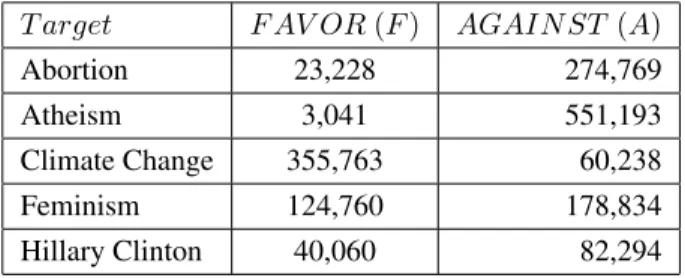
4.2 Collecting and Preprocessing Tweets
T arget F AV OR (F ) AGAIN ST (A) Abortion 23,228 274,769 Atheism 3,041 551,193 Climate Change 355,763 60,238 Feminism 124,760 178,834 Hillary Clinton 40,060 82,294
Table 2: Number of collected tweets per target and stance
As can be seen in Table 2, the collected tweets are very unevenly distributed between target-stance pairs. There are two causes for this: the uneven dis-tribution of different stances on Twitter in general, and uneven number of representative hashtags that we were able to associate with each target-stance pair. For instance, the pair “Climate Change is a Global Concern: AGAINST” was represented by only 15 tweets in the training data that was pro-vided, limiting us to only two representative hash-tags. Since our deep learning models require bal-anced amount of samples, we used the balancing technique described in the previous section.
To eliminate the possibility that resulting clas-sifiers would only learn the hashtags in the query,
we removed these hashtags from the majority of the collected tweets, keeping them only in 25% of the tweets.
4.3 Augmenting Data Using Word2Vec
Data augmentation techniques are widely used to enhance generalization of models with respect to input transformations that are known to not affect the output significantly. An example application of data augmentation in NLP can be found in (Zhang and LeCun, 2015), where they used thesaurus-based synonym replacement (WordNet (Fellbaum, 1998)) to generate additional training samples. We applied the technique used by Zhang et al (Zhang and Le-Cun, 2015) to our task, with the difference that we used Word2Vec (Mikolov et al., 2013) instead of a thesaurus to find similar words. The underlying in-tuition was that Word2Vec can provide better cover-age for phrases related to our targets.
The algorithm of the data augmentation is as fol-lows. At every step, we randomly selected a tweet from the non-augmented training set. We sampled a number r of words/phrases we would like to re-place from a geometric distribution with parameter p. We then randomly sampled r words/phrases, that are part of the Word2Vec vocabulary from the cur-rent tweet. (if r was larger than number of avail-able words/phrases n, we used r mod n.) For each of these words/phrases, we retrieved a list of most similar ones in terms of cosine similarity of Word2Vec vectors. We ordered the list in decreas-ing order of similarity and truncated it to not in-clude items with similarity less than threshold t. We then sampled index s of selected replacement from another geometric distribution with parameter q (again, we used modulo if s was too big). The original words/phrases were then replaced, and the tweet was added to the augmented dataset. The particular values of p, q and t were 0.5, 0.5 and 0.25 respectively. Using this method, we generated 500,000 extra tweets for each target-stance pair.
5 Evaluation
5.1 Baseline
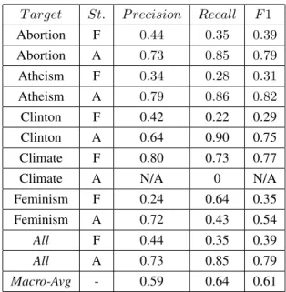
To have a better sense of our approach’s perfor-mance, we compared results against a simple base-line. We built a set of Naive Bayes classifiers us-ing bag-of-word features and optimized their
pa-rameters using 20-fold cross validation on origi-nal training data. We experimented with different thresholds on word count for a word to be included into vocabulary. We also set up separate thresholds for hashtags and at-mentions. After selecting the most promising values of thresholds, priors and the smoothing parameter, we ran the Naive Bayes clas-sifiers on the test data to obtain results shown in Ta-ble 3.
5.2 Validation Results
We trained the models using the collected dataset and validated them on the training set provided for the task. The validation results informed the choice between the word-level and the character-level clas-sifiers for each target. Without Word2Vec augmen-tation, character-level classifier achieved the best performance only for the target “Feminist Move-ment”. When Word2Vec augmentation was intro-duced, the character-level model achieved the best performance for the target “Climate Change” and the stance ”FAVOR” of the target ”Hillary Clinton”. The word-level model performed better for the tar-gets: “Legalization of Abortion”, “Atheism” and the stance ”AGAINST” of the target “Hillary Clin-ton”. We were able to achieve better average perfor-mance for the target ”Hillary Clinton” by combin-ing character-level and word-level classifiers with a simple heuristic: whenever character-level model
T arget St. P recision Recall F 1 Abortion F 0.44 0.35 0.39 Abortion A 0.73 0.85 0.79 Atheism F 0.34 0.28 0.31 Atheism A 0.79 0.86 0.82 Clinton F 0.42 0.22 0.29 Clinton A 0.64 0.90 0.75 Climate F 0.80 0.73 0.77 Climate A N/A 0 N/A Feminism F 0.24 0.64 0.35 Feminism A 0.72 0.43 0.54 All F 0.44 0.35 0.39 All A 0.73 0.85 0.79 Macro-Avg - 0.59 0.64 0.61
Table 3: Baseline performance (Naive Bayes classifiers, test data), St. - Stance
T arget St. P recision Recall F 1 P recision Recall F 1
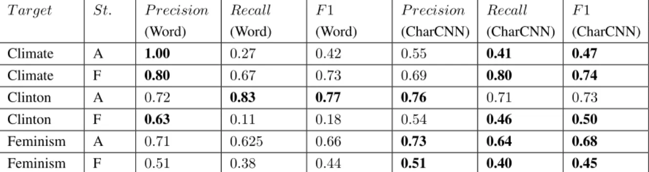
(Word) (Word) (Word) (CharCNN) (CharCNN) (CharCNN) Climate A 1.00 0.27 0.42 0.55 0.41 0.47 Climate F 0.80 0.67 0.73 0.69 0.80 0.74 Clinton A 0.72 0.83 0.77 0.76 0.71 0.73 Clinton F 0.63 0.11 0.18 0.54 0.46 0.50 Feminism A 0.71 0.625 0.66 0.73 0.64 0.68 Feminism F 0.51 0.38 0.44 0.51 0.40 0.45
Table 4: Performance of Word-Level Classifiers for Climate Change, Hillary Clinton and Feminist Movement.
predicts “AGAINST”, use that decision, otherwise resort to the decision of word-level model.
Table 4 compares the performance of the character-level and word-level classifiers for the tar-gets where character-level classifiers yielded an ad-vantage. The macro-average F1 validation score was 0.65.
5.3 SemEval Competition Results
Our model was able to achieve a Macro F-score of 0.6354 (placing us eighth out of 19 teams), while the best performing model had a Macro F-score of 0.6782. Table 5 details results on the test data for each target and stance.
T arget (rank) St. P R F 1 Abn. (1) F 0.54 0.67 0.60 A 0.86 0.54 0.66 Ath. (12) F 0.33 0.25 0.29 A 0.82 0.73 0.77 H. Cl (9) F 0.37 0.53 0.43 A 0.68 0.66 0.67 Cl. Ch. (12) F 0.80 0.82 0.81 A N/A 0 N/A Fem. (8) F 0.37 0.40 0.38 A 0.79 0.58 0.67 All (8) F 0.56 0.61 0.58 A 0.78 0.61 0.68 Macro-Avg - 0.67 0.61 0.635
Table 5: Results on test data, with rank out of the 19 teams.
6 Discussion and Future Work
An interesting result of our work was that given enough data, character-level models outperformed word-level models for tweet classification (with a
dramatic improvement in case of ”Hillary Clin-ton: FAVOR”). Due to the lack of data, it was necessary to resort to a data augmentation tech-nique to generate sufficient amount and diversity of data for character-level model to show its advan-tage. Another interesting finding from our work is the suitability of word2vec-based substitution as a data augmentation technique. As far as we know, word2vec has not previously been used for data aug-mentation in this manner.
As can be seen in Table 5, our system did not per-form too well for certain target-stance pairs (e.g., Atheism-Against). We hypothesize that the reason for this is the noise and the limited size of the col-lected training data. Thus, we believe that the per-formance of the system can be improved through better data expansion and cleaning techniques.
We see several avenues for future improvements. First, it might be beneficial to use unsupervised pre-training for our models (e.g., using autoencoders for Twitter (Vosoughi et al., 2016)). Second, data cleaning can potentially be improved using boot-strapping. This would entail using our current mod-els (optimized for high precision) to gather cleaner data for the second tier of models. It could be re-peated while validation performance improves. Fi-nally, because of the constraints of this SemEval task, we did not manually select hashtags or terms commonly associated with target-stance pairs. In-clusion of such hashtags can potentially boost the quality of the dataset, leading to better performance of our models.
References
Ronan Collobert, Jason Weston, L´eon Bottou, Michael Karlen, Koray Kavukcuoglu, and Pavel Kuksa. 2011.
Natural language processing (almost) from scratch. The Journal of Machine Learning Research, 12:2493– 2537.
Christiane Fellbaum. 1998. WordNet. Wiley Online Li-brary.
Ross Girshick, Jeff Donahue, Trevor Darrell, and Jiten-dra Malik. 2014. Rich feature hierarchies for accurate object detection and semantic segmentation. In Pro-ceedings of the IEEE conference on computer vision and pattern recognition, pages 580–587.
Geoffrey E Hinton, Nitish Srivastava, Alex Krizhevsky, Ilya Sutskever, and Ruslan R Salakhutdinov. 2012. Improving neural networks by preventing co-adaptation of feature detectors. arXiv preprint arXiv:1207.0580.
Marcus Hutter. 2002. Distribution of mutual informa-tion. Advances in neural information processing sys-tems, 1:399–406.
Diederik Kingma and Jimmy Ba. 2014. Adam: A method for stochastic optimization. arXiv preprint arXiv:1412.6980.
Tomas Mikolov, Ilya Sutskever, Kai Chen, Greg S Cor-rado, and Jeff Dean. 2013. Distributed representa-tions of words and phrases and their compositional-ity. In Advances in neural information processing sys-tems, pages 3111–3119.
Akiko Murakami and Rudy Raymond. 2010. Support or oppose?: classifying positions in online debates from reply activities and opinion expressions. In Proceed-ings of the 23rd International Conference on Compu-tational Linguistics: Posters, pages 869–875. Associ-ation for ComputAssoci-ational Linguistics.
Swapna Somasundaran and Janyce Wiebe. 2009. Rec-ognizing stances in online debates. In Proceedings of the Joint Conference of the 47th Annual Meeting of the ACL and the 4th International Joint Conference on Natural Language Processing of the AFNLP: Volume 1-Volume 1, pages 226–234. Association for Compu-tational Linguistics.
Matt Thomas, Bo Pang, and Lillian Lee. 2006. Get out the vote: Determining support or opposition from con-gressional floor-debate transcripts. In Proceedings of the 2006 conference on empirical methods in natural language processing, pages 327–335. Association for Computational Linguistics.
Soroush Vosoughi, Helen Zhou, and Deb Roy. 2015. Enhanced twitter sentiment classification using con-textual information. In 6TH Workshop on Computa-tional Approaches to Subjectivity, Sentiment and So-cial Media Analysis (WASSA 2015), page 16.
Soroush Vosoughi, Prashanth Vijayaraghavan, and Deb Roy. 2016. Tweet2vec: Learning tweet embeddings using character-level cnn-lstm encoder-decoder. In
Proceedings of the 39th International ACM SIGIR Conference on Research and Development in Infor-maion Retrieval. ACM.
Xiang Zhang and Yann LeCun. 2015. Text understand-ing from scratch. arXiv preprint arXiv:1502.01710.