An efficient 1D numerical model adapted to the study of transient convecto-diffusive heat and mass transfer in directional solidification

HAL Id: hal-01496974

https://hal.archives-ouvertes.fr/hal-01496974

Submitted on 28 Mar 2017

HAL is a multi-disciplinary open access

archive for the deposit and dissemination of

sci-entific research documents, whether they are

pub-lished or not. The documents may come from

teaching and research institutions in France or

abroad, or from public or private research centers.

L’archive ouverte pluridisciplinaire HAL, est

destinée au dépôt et à la diffusion de documents

scientifiques de niveau recherche, publiés ou non,

émanant des établissements d’enseignement et de

recherche français ou étrangers, des laboratoires

publics ou privés.

An efficient 1D numerical model adapted to the study of

transient convecto-diffusive heat and mass transfer in

directional solidification

Virgile Tavernier, Séverine Millet, Daniel Henry, Valéry Botton, Ghislain

Boutet, Jean-Paul Garandet

To cite this version:

Virgile Tavernier, Séverine Millet, Daniel Henry, Valéry Botton, Ghislain Boutet, et al.. An efficient

1D numerical model adapted to the study of transient convecto-diffusive heat and mass transfer in

directional solidification. International Journal of Heat and Mass Transfer, Elsevier, 2017, 110,

pp.209-218. �10.1016/j.ijheatmasstransfer.2017.03.021�. �hal-01496974�

Published in International Journal of Heat and Mass Transfer 110 (2017) 209–218

http://dx.doi.org/10.1016/j.ijheatmasstransfer.2017.03.021

An efficient 1D numerical model adapted to the study of transient

convecto-diffusive heat and mass transfer in directional solidification.

Virgile Tavernier

, Séverine Millet

, Daniel Henry

, Valéry Botton

, Ghislain Boutet

, Jean-Paul

Garandet

1

Laboratoire de Mécanique des Fluides et d’Acoustique, CNRS/Université de Lyon, Ecole Centrale de

Lyon/Université Lyon 1/INSA de Lyon, ECL, 36 avenue Guy de Collongue, F-69134 Ecully Cedex,

France

2

INSA Euro-Méditerranée, Université Euro-Méditerranéenne de Fès, Route de Meknès, BP 51, 30000

Fez, Morocco

3

Telespazio France, 26 avenue J.F. Champollion, B.P. 52309 - 31023 Toulouse Cedex 1, France

4

CEA, Laboratoire d’Instrumentation et d’Expérimentation en Mécanique des Fluides et

Thermohydraulique, DEN/DANS/DM2S/STMF/LIEFT, CEA-Saclay, F-91191 Gif-sur-Yvette Cedex,

France

Abstract

We combine an effective diffusivity model with a numerical approach initially proposed by Meyer (1981) to simulate transient heat and mass transfer phenomena in a directionally solidifying Sn-Bi rod. This particularly efficient 1D numerical model is light enough to be used within the frame of optimization methods at reasonable numerical cost. This approach is tested against reference in situ measurements obtained under microgravity conditions during the Mephisto program. We simulate the final homogenization transient of several experimental runs with different pulling velocities. The solid/liquid interface temperature evolution with time is extracted from the simulations and compared with that obtained by Seebeck in line measurements. After optimization of the model the observed discrepancy between the simulated and measured data is less than 1.5%. This validates both the proposed very efficient 1D numerical approach and the consistency of the set of thermophysical parameters values for dilute Sn-Bi alloys.

Keywords:

Segregation; Effective diffusion; Crystal growth; Thermophysical parameters; Seebeck.

I.

Introduction

Directional solidification, where a molten alloy is frozen from one end, is a process with numerous industrial applications in the fields of crystal growth and metallurgy. The case where the solidification rate is controlled in order for the solid liquid front to remain planar, i.e. avoiding cells or dendrites and bulk nucleation to occur, is in particular relevant to crystal growth applications. From a mathematical standpoint, this can be considered as a model transport problem, where the position of the solid liquid interface cannot be a priori prescribed, but results from time dependent boundary conditions. In addition, the problem is both multiphysics since the alloy thermodynamic state is ruled by a phase diagram coupling the alloy local composition to its temperature and multiscale since the diffusivities associated to heat and concentration take usually very different values. Last but not least for our present purposes, the transport in the melt part of the alloy is usually influenced by the presence of convection due to buoyancy effects. It is thus an intricate problem.

The continuous development of computational resources and the need for a better understanding of the phenomena and for optimization of industrial processes have led to the development of several numerical modelling strategies in the last decades. Numerous efforts have been made to develop realistic 2D and 3D simulation tools using either an enthalpy approach featuring a diffuse interface computed on a fixed mesh [1– 5] or resorting to adaptive meshing techniques to track the solidification front and insure its fine description with nodes located on the interface [6–11]. Combining coupled 2D and 3D simulations is now an established

2

strategy to reduce computational cost in particular in the Czochralski configuration in which the front is nearly fixed in space [12,13]. However, the computational time associated with such simulations still goes from several hours to several days. As a consequence it is prohibitive to include these models within optimization procedures based on parametric minimization strategies. There is thus still a real need of still lighter models, typically 1D, to perform fast computations of directional alloys solidification in convecto-diffusive conditions.

Meyer [14] proposed an original technique allowing to efficiently solve the coupled heat and mass transfer problem. This technique has been shown to give reliable results [15,16] and the short computational time associated with this method offers the possibility to implement it within a parametric optimization procedure. Yet, Meyer’s method only considers diffusive situations and it would be interesting to extend this method to account for convective effects. Such an extension is proposed in the present paper, based on an effective diffusivity formalism in order to keep the 1D approach. A second step is to test the ability of this modified Meyer method to account for the global consistency of a reference experimental dataset obtained in microgravity by directional solidification of tin bismuth alloys in the MEPHISTO apparatus [17,18]. A specificity of the featured data is that it is not restricted to a limited number of post-mortem concentration vs position measurements, as is often the case in metallic alloys and semiconducting materials. Indeed, what is measured during the experiments is the real time Seebeck signal associated with the growth interface temperature. We thus have access to an almost continuous composition vs time data set. Another feature of our experimental data is that it was obtained in microgravity, i.e. in conditions of relatively weak convective transport and, in any case, devoid of turbulent fluctuations. Note finally that the simulations with the modified Meyer method require thermophysical data, which, for Sn-Bi, are still difficult to obtain.

To sum up, the objectives of our study are threefold: to propose significant improvements of Meyer’s method, with the introduction of an effective diffusion approach in order to extend this method to convecto-diffusive problems and the use of specific numerical techniques in order to insure a second order spatial scheme; to present yet unpublished reference experimental results obtained in microgravity, which will be used to test the potentiality of the modified Meyer method; to show the consistency of a set of thermophysical parameters values published separately in former papers and which will be used in the simulations.

Section II is dedicated to the background of the present paper, including a brief presentation of Meyer’s method, of the relevant physical phenomena and of the experimental set up and growth conditions. We then proceed in section III to a description of the proposed modified Meyer’s method and boundary and initial conditions, before turning to some specificities of its numerical implementation in section IV. Section V is devoted to the comparison with the experimental data before a conclusion in section VI.

II.

Background

2.1 Meyer’s original method

The equations to be solved to describe a one-dimensional solidification process with moving interface in the diffusive regime are those associated with the conservation of heat and impurity concentration. If we use the subscripts + and - to denote the liquid and solid phases, respectively and the subscript int to denote the interface, we can write the following equations for temperature and impurity concentration :

Heat conservation equation

(1)

Heat conservation at the interface

(2)

Temperature continuity at the interface

(3)

3

Impurity conservation at the interface

(5)

Phase diagram relation

(6)

In these equations, is the thermal conductivity, is the thermal capacity, is the density, is the latent heat of fusion, and is the solutal diffusivity.

To solve this problem known as the Stephan problem, a numerical method was proposed by Meyer [14]. New variables are first introduced, and , which correspond to the heat and impurity

fluxes, respectively. The temperature and impurity concentration can be defined with these new variables as: (7)

and

(8)

respectively. The problem is discretized in time with a time step and we want to calculate the solution and at time (with ) from and . The functions and , and and are then solutions of ordinary differential equations:

(9) with and , (10) with and , and

(11) with and , (12) with and .

The functions , , and correspond to the temperature and concentration boundary conditions applied on the extremities of the sample ( and ) at each time. For the case presented in this paper, the boundary conditions for temperature are obtained in each phase from the expressions (20), (28) and (29) introduced later in the paper, and the boundary conditions for concentration are obtained from the concentration in each phase far from the interface (respectively and given in Table 1).

To get the temperature and concentration fields, the functions and still have to be determined. They are solutions of the following equations derived at order 1 in time from the conservation equations: (13) and

4

(14)

At each time step, the solutions are calculated from the boundary conditions taken at the solid/liquid interface: (15) and (16)

The values of and are obtained by solving a system of two equations deduced from heat and mass

conservation at the interface:

(17) (18)

Finally, at each time step, once the functions and , and , and and have been calculated, the temperature and concentration fields in the sample can be obtained from equations (7) and (8) above. As a conclusion, the interest of this 1D method is thus to substitute the set of coupled partial differential equations ruling the moving front problem by a set of ordinary differential equations with initial conditions.

2.2

The Mephisto experimental program

The Mephisto program was conducted in the eighties and nineties by the French spatial agency (CNES) and the French atomic research center (CEA) in collaboration with the American space agency (NASA) and various American labs. The objectives were to perform solidification experiments of metallic alloys in micro-gravity, in order to avoid perturbing convective effects, in carefully controlled experiments reaching nearly purely diffusive species transport regime. Among the investigated problems, one can cite the morphological stability of a planar front, g-jitters effects in microgravity conditions or the determination of liquid phase thermophysical properties, see e.g. [17–19]. Mephisto was part of a larger material science effort, see e.g. [20,21] in the frame of the ambitious United States Microgravity Payloads (USMP) program that featured different campaigns in connection with flight opportunities between 1992 and 1997. Specifically regarding Mephisto, the data that will be discussed in the frame of the present paper are issued from two flights, namely USMP1 in 1992 and USMP3 in 1996, featuring tin bismuth alloys and where the Mephisto device was operated under CEA scientific leadership. The nominal alloy compositions for the feed materials were at.% Bi and 1.6 at.% Bi for the USMP1 and USMP3 flights, respectively, meaning that the alloys could be considered as dilute. The starting materials were synthesized in the CEA laboratory from 6N tin and bismuth sources.

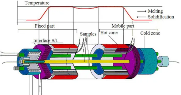
Briefly speaking, Mephisto is a sophisticated Bridgman furnace, with two heating and cooling sub-systems, where three separate elongated (length = 850 mm, diameter = 6 mm) cylindrical samples are solidified in parallel (see the sketch in Fig. 1). Sample #1 is dedicated to a measurement of the Seebeck thermoelectric signal, which is used to obtain most of the experimental data presented here. From a thermoelectric standpoint, the solid-liquid-solid sample behaves like a double thermocouple. One of the interfaces is maintained at a given position during the experiment to provide a reference temperature value, namely that of the liquidus at the nominal composition of the alloy. This temperature can be matched with the contribution coming from the other interface, whose motion is controlled by an imposed displacement of the heating-cooling sub-system. Such a differential measurement is rendered necessary by the small amplitude of the observed signals, ranging from 0.5 to 10 µV for the tin based alloys used within the frame of the Mephisto program.

5

As mentioned earlier, this Seebeck diagnostic allows data to be gathered from various growth conditions on a single piece of material, a useful feature in the space environment where samples are obviously scarce. To accomplish this, the experiment is organized in cycles, that consist of (i) a solidification stage at a prescribed velocity over a given length, sufficient to form the solute boundary layer ahead of the growth front and to reach steady state conditions, (ii) a stabilization period to re-homogenize the melt, (iii) a re-melting of the previously solidified material, and (iv) another stabilization period before the subsequent cycle. In some cases, stages (iii) and (iv) are not carried out, so that the frozen solute distribution can be a posteriori analyzed by classical metallurgical techniques after the samples have been brought back to earth.

Let us discuss now what is measured by the Seebeck signal. First, as a consequence of thermoelectric effects, the measured electrical tension between the ends of the sample is directly proportional to the temperature difference between the two isothermal solid/liquid interfaces. More precisely, the observed electrical signal can be written as:

where represents the effective thermoelectric power coefficient (µV/K) between the liquid and solid

phases, and standing for the temperatures of the moving and reference fixed interfaces, respectively.

At a given growth velocity, the Seebeck signal should in principle be measurable directly as a function of time. Unfortunately, even though the data is sampled continually, a one to one correspondence with the interface temperature variation cannot be simply identified due to a drift in the thermoelectric signal, associated with the position of the interface within the furnace. This drift is likely due to the existence of concentration and microstructure gradients within the formed solid, that lead to the development of thermoelectric currents as growth proceeds [22]. Thus, in order to extract meaningful information, we always had to rely on events that caused a well-defined Seebeck signal variation at a given furnace position. For our present purposes, the special growth event is the end of the pulling stage: as the variation of the front position during the final transient is always smaller than a millimeter, the associated Seebeck drift can be safely neglected. What will be analyzed in the frame of the present paper is thus the data associated with the re-homogenization of the solute accumulated within the boundary layer ahead of the growth front, for which the one to one correspondence between the Seebeck signal and the interface temperature can be taken for granted.

An important feature of the thermoelectric coefficient is that it cannot be a priori assumed to be independent of the interface composition, even for the dilute alloys considered in the experimental program. This is due to the very high thermoelectric power of Bi. We are not, however, in a position to prescribe a closed form relation for such a variation. The comparison between experimental and numerical data will thus be done assuming a constant effective thermoelectric coefficient for each re-homogenization stage, but we shall a

posteriori check that the ranges of variations of such effective thermoelectric coefficients follow a monotonic

trend and remain within reasonable bounds.

As for the two other samples present in the furnace, a measurement of the electrical resistance is performed on sample #2. When the different resistivities of the base material, either solid or liquid, are taken into account, this measurement can be translated in an estimation of the solidification velocity. In addition, sample #2 contains thermocouples for the measurements of the temperature gradients within the alloy. Sample #3 is for Peltier pulse marking and post-mortem analysis of the shape of the quenched growth interface. Sample #3 also contains thermocouples for temperature gradient measurements.

It should be noted that the experimental device exhibits some thermal inertia leading to a delay of the thermal gradient inside the sample with respect to that imposed by the furnace. This implies that the thermal gradient in the sample will continue to move after the furnace motion has been stopped, until both gradients eventually match. This phenomenon particularly occurs in the re-homogenization period. If the delay is characterized by the time , the changes that will affect the effective temperature profile imposed along the sides of the

sample can be modeled by a decreasing exponential law [23] given by:

(20)

where is the temperature profile at the end of the solidification phase, is the thermal gradient in the sample around the interface ( K/cm and K/cm for USMP3, and K/cm and

6

K/cm for USMP1) and is the pulling rate of the furnace in steady regime. Based on the experiments, the thermal delay has been estimated to .

Figure 1: Schematic of the Mephisto furnace, showing the implementation of the three samples within the fixed and mobile parts. The solid-liquid interface is located between the hot and cold zones. The characteristic temperature profile, as given by the position of the hot and cold zones is also indicated, along with the directions of melting and solidification.

In connection with the objective of the present paper, it should be noted that former publications carried out 2D/3D numerical simulations of the Mephisto device [24,25]. In these papers, the set of chosen thermophysical parameters values has been fixed to realistic values. Unfortunately no comparison with in situ Seebeck measurements are given in these articles and no comparison of final transient with experiments are proposed.

III.

Relevant physical phenomena

The first issue to be discussed concerns the fact that, even in microgravity conditions, the possibility of convective solute transport cannot be ruled out, especially because the liquid phase molecular diffusion coefficients are very low, in the 10-9 m2s-1 range. As a matter of fact, the weak but non negligible effect of natural buoyancy driven convection, coming from the interaction of density gradients with gravity, was clearly demonstrated in the frame of the Mephisto program [18,26]. A good description of the re-homogenization phase kinetics thus requires addressing the problem. This was done in a number of papers [27–30], where it was shown that an effective diffusion coefficient, accounting for the additional solute transport, could be defined. More precisely, thanks to an order of magnitude analysis, this effective diffusion coefficient can be defined as:

(21)

where is the distance to the interface in the liquid part (taken as ), is the diameter of the

sample, and is a characteristic value of the convective velocity at the distance , derived for a horizontal two-dimensional cavity submitted to a horizontal temperature gradient and defined as:

(22)

7

(23)

with an estimate of the average ‘steady’ residual gravity level and the thermal expansion coefficient. The free parameter  will be adapted to match the numerical results with the experimental results ( corresponds to the purely diffusive case). is equal to at the interface (rigid wall where ) and

increases with the distance to the interface. Note that the expression of is valid for between 0 and , where it matches an analytical 1D solution to the 2D planar Navier Stokes equations [31]. As a consequence, the expression of will, as well, be used for between 0 and , and the value obtained at will be

used in the rest of the liquid sample. It should be noted that the measurement of the residual gravity aboard a space vessel is a formidable task, since a number of quasi-steady (e.g. residual drag) or transient (e.g. maneuvers) components have to be considered. Quantifying precisely their contribution to the effective diffusion of species is also challenging (see for instance [32] for a discussion on the subject). Nevertheless, regarding the averaged effect of interest in the frame of the present paper, it can be safely stated that it should be comparable to the effect of a steady component with 1 µg0 intensity, with g0 standing for gravity on earth

(g0 = 9.81 ms-2).

Regarding the thermophysical parameters, further assumptions are required. The first one is that potential variations of heat and mass diffusivities with the alloy composition can safely be neglected since the experiment features dilute alloys. The same applies to the liquidus and solidus slopes in the phase diagram relation, Eq. (6), which can be taken as a simple linear relation:

(24)

where represents the melting temperature of pure tin ( °C). As a consequence, the phase diagram information can also be written as with standing for the partition coefficient of Bi in Sn, also constant in the composition range to be investigated. The relevant thermophysical parameters for dilute tin bismuth alloys will be taken as: for the partition coefficient, K/(at.% Bi) for the liquidus slope, W/(m K) and W/(m K) for the thermal conductivities, J/(kg K) and J/(kg K) for the thermal capacities, kg/m3 and kg/m3 for the mass densities,

_{m²/s [33,34] and m²/s for the Bi diffusion coefficients, J/kg for the}

latent heat of fusion, K-1 for the thermal expansion coefficient, m²/s for the kinematic viscosity. As for the thermoelectric coefficient, tentative values of µV/K, µV/K

and µV/K were proposed, respectively for pure tin [35], and alloys with 0.58 at.% Bi [22] and 1.6 at.%

Bi [23]. However, as mentioned earlier, due to the significant variability of with the Bi content, we will allow

the values of the thermoelectric coefficient to be taken as variable in the optimization procedure.

Finally, the issue of the initial condition, i.e. the state at the end of the steady solidification regime for our present re-homogenization problem, also needs to be discussed. Regarding the solutal problem, we first have to know if the initial transient leading to the steady regime is really completed. An analytical solution for the extent of this initial transient in purely diffusive solute transport conditions had been given long ago by Smith et al. [36]. We can then estimate the characteristic length of the initial transient using this analytical solution and compare it with the length solidified before the re-homogenization process. For 7D, 8B and 11C2 experiments in the USMP3 campaign, the solidified length is respectively about 5.5 times, 3.5 times and 4.5 times the characteristic length of the initial transient. Moreover, in convecto-diffusive solute transport conditions, numerical simulations and order of magnitude arguments show that the initial transient should be shorter, since the boundary layer ahead of the interface is reduced [37]. In this respect, we can reasonably think that for 8B and 11C2 experiments, the experimental initial transient is shorter than the one estimated with the analytical solution, corresponding to a still more favorable situation. Thus, we can consider that the initial transient is fully completed and that the steady-state solute profile can be safely taken as the initial condition for the simulations. We have also to take into account the fact that the initial state may be affected by residual convection for the thermal problem. Nevertheless, as Sn-Bi is a good thermal conductor, the temperature profile can be considered as diffusive with linear profiles in each phase (with the constant gradients and defined previously), taking as reference the interface temperature . can then be

written as:

8

where is used for the liquid part (i.e. ) and for the solid part (i.e. ). Concerning the

concentration profile, it is taken uniform within the computational domain in the solid phase at a given concentration which needs to be assessed. Once this is done, is used to determine the initial composition profile within the fluid ahead of the interface defined in convecto-diffusive situations as:

(26) where is the thickness of the solute boundary layer connected to by the following formula [38]:

(27) For a number of experiments, respectively referred to as 7D, 11C2 and 11I (see Table 1), we do have composition measurements and we are thus in a position to fill in an experimental input for , from which is obtained using (27) and the composition profile within the fluid using (26). Interestingly, for the higher pulling rates 7D and 11I, , meaning that purely diffusive transport conditions were achieved in the solidification stage. In contrast, for the 11C2 experiment, is significantly smaller than , meaning that residual convection did have an influence. This is not unexpected, since it is well known that the sensitivity to residual convection is smaller at higher pulling rates [26]. There exists another possibility to determine the initial composition profile, particularly useful when is not available. In that case, is first estimated using a characteristic equation derived in [38], is deduced using (27) and the composition profile within the fluid is then obtained using (26). This alternative procedure has been tested for the different USMP1 and USMP3 experiments: the relative error between the estimated and measured values of was found to be less than 0.5%, indicating the reliability of this alternative procedure. This procedure was then used for the 8B experiment, where we do not have any measured value because the solidified sample has been re-melted, and the value of was thus estimated at 1.54 Bi at.% (see Table 1).

Experiment Experimental Campaign Nominal (Bi at.%) Steady (Bi at.%) Pulling rate (µm/s) Re-homogenization duration (s) 7D USMP3 1.6 1.6 (m) 2.24 7200 8B USMP3 1.6 1.54 (e) 1.04 10800 11C2 USMP3 1.6 1.3 (m) 0.47 21600 11I USMP1 0.58 0.58 (m) 5.2 7200

Table 1: Characteristics of the considered Mephisto experimental runs. For , some values are measured (m) or estimated (e).

Concerning the boundary conditions, they are given for the temperature by the expression (20) applied on the extremities of the sample ( for the liquid part and for the solid part) at each time. In order to obtain these boundary conditions, the temperature values on the extremities of the sample at the end of the solidification stage, which have to be introduced in the expression (20), are derived from (25) and taken as:

(28)

(29)

For the concentration, the sample is considered as long enough to keep the initial concentrations and unchanged at the far ends of the liquid and solid zones, respectively.

IV.

Numerical developments

As our sample is cylindrical, with a small diameter, namely 6 mm and the pulling rates remain moderate, we can assume that the solidification front is planar both at the microscopic (no cells or dendrites) and the macroscopic (negligible curvature) scales so that the problem can be treated in a one-dimensional approximation. The method proposed by Meyer can then be used. This method was implemented in MATLAB in order to simulate the re-homogenization transient phenomena in the considered Sn-Bi samples. Only a portion of the very long experimental samples (40 mm compared with the overall 850 mm), on both sides of

9

the interface, is considered. The simulated sample, liquid in its left part and solid in its right part, is discretized by a grid of uniformely distributed points distant by and located at .

At each time step, the solutions of the spatial ordinary differential equations giving and , and , and and are obtained through a one-step implicit Adams-Moulton scheme, which has the advantage to be unconditionally stable and of order 2. For the functions and , and then and , the calculations progress from the boundary conditions applied at the ends of the sample. In contrast, for and , calculated values at the interface are used to initiate the computations. A precise calculation of the interface position, generally not located on a grid point, is then needed, as well as a precise initiation of the one-step implicit Adams-Moulton scheme for and at this interface position.

To calculate the position of the interface from equations (17) and (18) at a given time step, we first use its position at the previous time step and define two grid points and at a certain distance on both sides of this interface ( ). The calculations in the liquid phase and solid phase are then done in

extended domains, on grid points from to and from to , respectively. The values of and

are then evaluated for supposed values of taken on the grid points between and , allowing to find

the two neighboring points between which the function crosses zero. The position of the interface,

which corresponds to , is then deduced by a three points quadratic interpolation using two points in the solid phase and one in the liquid phase.

The position of the interface is then used to interpolate , , and at the interface. These values are required to obtain and (Eqs. (15) and (16)), which are then used as initial

conditions for the calculation of and . To keep the second order for this calculation, a specific method is used, as illustrated in figure 2. In this figure, denotes any function defined as on fixed grid points, with a known value at the moving interface, as it is

the case for and in this paper (Eqs. (13) and (14)). Because the interface position is not located on a grid point, we do not use the previous relation between and at the interface, so that the one-step implicit Adams-Moulton scheme is not adapted to initiate the calculation. A specific scheme is thus constructed, which allows to get the values of at the first three grid points on both sides of the interface: two forward second order explicit Nyström scheme steps and one backward second order explicit Adams-Bashforth scheme step, adapted to the locally non-regular mesh, are performed simultaneously, leading to three variables linear systems, which are easily solved. The classical one-step implicit Adams-Moulton scheme is then used for the other grid points. Let us underscore that this numerical approach is a key ingredient to insure the global precision of the scheme with a reasonable computational time.

10

on fixed grid points, with a known value at the moving interface. For both sides of the interface, the steps (I), (II) and (III) are performed simultaneously, leading to three variables linear systems, which are then solved. The steps (I) and (II) are both second order explicit Nyström scheme steps providing relations between , and , and between , and , respectively, as an example for the solid part. The step (III) is a second order explicit Adams-Bashforth scheme step providing a relation between , , and , as an example for the solid part.

As an illustration, typical computed longitudinal concentration profiles obtained from our code are plotted in figure 3, corresponding to the 7D experimental run in diffusive conditions. The time evolution of this profile (up to 6000 sec) allows the visualization of the interface displacement during the re-homogenization transient.

Figure 3: Time evolution of the longitudinal concentration profile in the 7D experiment obtained by simulation using the purely diffusive transient model ( ). The concentration profile used as an initial condition for the simulation (i.e. at 0 sec) is plotted with blue dashed line, and the concentration profiles corresponding to 600 sec, 2400 sec and 6000 sec are plotted with red dotted line, magenta dashed-dotted line and black solid line, respectively. The solidification occurs from right to left.

V.

Comparison with the experiments

5.1 Fit methodology

In each case shown in Table 1, the real-time Seebeck signals registered during the experiment are available. Such experimental signals can be seen in figure 4. The comparison with the numerical results will be first done qualitatively by comparing the Seebeck curves. To also have a better estimation of the discrepancy between the experimental and numerical results, we will also calculate an error criterion, Err, based on the norm and defined as:

(30)

where is the Seebeck signal at time . This Err criterion will also be used as an objective function to be minimized in the convecto-diffusive model for adjusting its tunable parameters.

5.2 Fit results

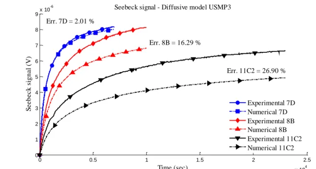
The simulations are first performed with the purely diffusive transient model ( ) for the different USMP3 Mephisto experiments. The results obtained by simulation with the purely diffusive transient model are compared with the experimental results in figure 4 for the 3 pulling rates. In each case, we see that the

0.02 0.022 0.024 0.026 0.028 0.03 0.032 0.034 0.036 0.038 0 1 2 3 4 5 6 x (m) C o n c e n tr a ti o n ( % a t. B i)

Time evolution of the concentration profile in 7D experiment Initial condition for concentration profile

Concentration profile at 600 sec Concentration profile at 2400 sec Concentration profile at 6000 sec

11

Seebeck signal strongly evolves with time during the re-homogenization period, due to the change of the interface temperature from its value in the steady regime (associated with and ) to its value in the rest state (associated with and ). The comparison between the experimental and numerical results is fairly good for one of the experiments, namely 7D, and rather bad for the others. The associated error criteria Err are 2.01%, 16.29%, and 26.90% for the 7D, 8B, and 11C2 experiments, respectively. It is thus shown that the 7D experiment can be well described by a purely diffusive transient model: this experiment has in fact the strongest pulling rate and is consequently expected to be the less sensitive to convective phenomena. In contrast, the 8B and 11C2 experiments cannot be properly described by the purely diffusive transient model and taking into account the convection then appears necessary.

Figure 4: Time evolution of the Seebeck signal recorded in the Mephisto USMP3 experiments during the re-homogenization period, compared to the results obtained by simulation using the purely diffusive transient model ( ).

As a second step, we want to adjust simultaneously the 7D, 8B and 11C2 experiments with simulations using the convecto-diffusive model presented in section III. This model involves the Grashof number , which has been calculated with a very low residual gravity , and has a free parameter , which is tuned to get the best fit between the curves. This optimization is based on the previously defined Err criterion measuring the discrepancy between the numerical and experimental Seebeck curves. Let us recall that the simulation results are first expressed in terms of concentration and temperature fields. An additional parameter has thus to be used to convert them into Seebeck curves, namely the Seebeck coefficient, . This

coefficient has a great influence on the calculation of the Seebeck curves, so that we chose to perform the optimization with two adjustable parameters, the coefficient and the Seebeck coefficient. Moreover, the few values found in the literature ( µV/K, µV/K and µV/K respectively for pure tin

[35], and alloys with 0.58 at.% Bi [22] and 1.6 at.% Bi [23]) show that this coefficient might decrease when the concentration is increased. In the optimization process, the value of was chosen to be the same for 7D, 8B and 11C2 experiments, whereas the Seebeck coefficient was separately optimized for each experiment.

The results obtained with the convecto-diffusive model are shown in figure 5. We see that the fits between the experimental curves and the simulated curves are rather good, with errors equal to 1.31%, 1.38%, and 1.49 % for the 7D, 8B, 11C2 experiments, respectively. These are very small values indeed considering the existing error bars on the numerous physical parameters values in this problem. These optimizations correspond to a coefficient and to values of the Seebeck coefficient equal to 1.079 µV/K (7D experiment), 1.208 µV/K (8B experiment), and 1.299 µV/K (11C2 experiment). These values of the Seebeck coefficient seem reasonable and their monotonic increase is consistent with the decrease in concentration at steady state (1.6, 1.54, and 1.3 Bi at.%, respectively, see table 1). Concerning the coefficient, it can be seen as a pre-factor of the squared convective velocity in expression (21) for the effective diffusivity . As the velocity is proportional to

the Grashof number, which is calculated with a residual gravity level of , the value can also be

0 0.5 1 1.5 2 2.5 x 104 0 1 2 3 4 5 6 7 8 9x 10 -6 Err. 7D = 2.01 % Err. 8B = 16.29 % Err. 11C2 = 26.90 % Time (sec) S e e b e c k s ig n a l (V )

Seebeck signal - Diffusive model USMP3

Experimental 7D Numerical 7D Experimental 8B Numerical 8B Experimental 11C2 Numerical 11C2

12

seen as a modulation of the gravity which would reach _{, a reasonable value for experiments in}

space, specially taking into account that the convective velocity field was derived using an approximate solution of the 2D planar Navier-Stokes equations. In addition, it should be recalled at this point that the procedure leading to equation (21) is based on an order of magnitude analysis, meaning that the value can clearly be taken as reasonable.

Figure 5: Time evolution of the Seebeck signal recorded in the Mephisto USMP3 experiments during the re-homogenization period, compared to the results obtained by simulation using the convecto-diffusive model (adjustment of the coefficient and of the Seebeck coefficient).

As a third step, we want to adjust the 11I experiment (from the USMP1 campaign) with the convecto-diffusive model using the coefficient value provided by the previous simulation. The Seebeck coefficient is separately optimized for this experiment. The result, corresponding to a Seebeck coefficient value equal to 1.343 µV/K, is shown in figure 6. We see that the fit error between the experimental curve and the simulated curve is equal to 1.07%, which is comparable to the errors obtained from the USMP3 simulations.

Figure 6: Time evolution of the Seebeck signal in the Mephisto USMP1 11I experiment during the re-homogenization period, compared to the result obtained by simulation using the convecto-diffusive model (adjustment of the Seebeck coefficient; the coefficient is determined from the USMP3 simulations).

0 0.5 1 1.5 2 2.5 x 104 0 1 2 3 4 5 6 7 8 9x 10 -6 Err. 7D = 1.31 % Err. 8B = 1.38 % Err. 11C2 = 1.49 % Time (sec) S e e b e c k s ig n a l (V )

Seebeck signal - Convecto-diffusive model USMP3

Experimental 7D Numerical 7D Experimental 8B Numerical 8B Experimental 11C2 Numerical 11C2 0 1000 2000 3000 4000 5000 6000 7000 8000 0 0.5 1 1.5 2 2.5 3 3.5 4 4.5x 10 -6 Err. 11I = 1.07 % Time (sec) S e e b e c k s ig n a l (V )

Seebeck signal - Convecto-diffusive model USMP1

Experimental 11I Numerical 11I

13

The value of the Seebeck coefficient obtained for this simulation seems reasonable and in accordance with the monotonic variation over the concentration mentioned above. The validity of this convecto-diffusive model and the consistency of the thermophysical parameters values are thus confirmed by comparison with experimental runs from two different campaigns.

VI.

Conclusion

This paper presents a very consistent and efficient 1D model for the longitudinal convecto-diffusive time dependent heat and mass transfer effects in a crystal growth experiment. This model has been tested on its ability to simulate final transients during which solute re-homogenization occurs. It reproduces the interface temperature temporal evolution in four experimental runs of the Mephisto microgravity program, featuring significantly different pulling velocities. Let us recall that, despite the apparent simplicity of the presented model, the considered physical problem is rather complex: it is a moving front problem, with phase change and impurity segregation, coupled with a 3D weakly unsteady natural convection flow in a very elongated cavity.

Modelling these microgravity experiments, performed several years ago, has required a consistent set of thermophysical parameters values, which has been available only in recent times. Another key ingredient is the numerical efficiency of the developed 1D convecto-diffusive model combining Meyer’s approach and the introduction of an effective diffusivity accounting for convection effects. The implemented second order scheme made it possible to introduce the numerical model within an optimization procedure at very reasonable computational cost. Though not technically impossible, performing a direct numerical simulation of such a complex physical problem case and running it numerous times for the sake of the optimization procedure would have been very costly indeed from a numerical standpoint.

The model features two adjustable parameters. One, referred to as , is introduced to account for both the uncertainty on the effective residual gravity level and the order of magnitude nature of the effective diffusivity approach. After numerical optimization, the adjusted value of  is 30, a compatible value with reasonable microgravity level. The other parameter is the Seebeck coefficient itself, which, in the same time, has a significant uncertainty and a strong influence on the result. After numerical optimization, the adjusted values are consistent with the expected decreasing monotonic behavior of with concentration and with the

range of values expected from literature. Finally, the observed discrepancy between the computed and measured composition data is less than 1.5%, an unexpectedly small value indeed when considering the number of parameters entering this problem and their respective uncertainties. We can thus confidently conclude on both the validity of this very efficient numerical approach and the consistency of the thermophysical parameters values.

Potential outlooks for applications of the method to new situations will require a determination of the value of . It can be either estimated in an order of magnitude approach [30, 34, 39] for known conditions (such as geometry, gravity, thermal expansion coefficient), or computed using a CFD approach in a simpler liquid phase configuration, without having to bother with the phase diagram coupling issues. Note that this efficient 1D model will be particularly valuable in a system scale process approach, giving the opportunity to numerically optimize a set of control parameters, once has been calibrated in a given specific experimental configuration, either under microgravity or on earth.

Acknowledgement

Virgile Tavernier held a doctoral fellowship from la Région Rhône-Alpes.

References

[1] M.P. Bellmann, M. M’Hamdi, Effect of flow pattern on the segregation of impurities in vertical Bridgman growth of multi-crystalline silicon, Journal of Crystal Growth. 362 (2013) 93–98.

doi:10.1016/j.jcrysgro.2011.10.055.

[2] M.P. Bellmann, B. Panjwani, M. Syvertsen, E.A. Meese, Dynamic simulation of impurity transport and chemical reactions in a Bridgman furnace for directional solidification of multi-crystalline silicon, Journal of Crystal Growth. 369 (2013) 47–54. doi:10.1016/j.jcrysgro.2013.02.008.

14

[3] M. Cablea, K. Zaidat, A. Gagnoud, A. Nouri, Y. Delannoy, Directional solidification of silicon under the influence of travelling magnetic field, J. Cryst. Growth. 401 (2014) 883–887.

doi:10.1016/j.jcrysgro.2014.11.062.

[4] M. Cablea, K. Zaidat, A. Gagnoud, A. Nouri, G. Chichignoud, Y. Delannoy, Multi-crystalline silicon solidification under controlled forced convection, Journal of Crystal Growth. 417 (2015) 44–50. doi:10.1016/j.jcrysgro.2014.07.042.

[5] R. Boussaa, L. Hachani, O. Budenkova, V. Botton, D. Henry, K. Zaidat, H. Ben Hadid, Y. Fautrelle, Macrosegregations in Sn-3 wt%Pb alloy solidification: Experimental and 3D numerical simulation investigations, International Journal of Heat and Mass Transfer. 100 (2016) 680–690.

doi:10.1016/j.ijheatmasstransfer.2016.04.120.

[6] S. Dumitrica, D. Vizman, J.-P. Garandet, A. Popescu, Numerical studies on a type of mechanical stirring in directional solidification method of multicrystalline silicon for photovoltaic applications, Journal of Crystal Growth. 360 (2012) 76–80. doi:10.1016/j.jcrysgro.2012.01.011.

[7] Y. Delannoy, F. Barvinschi, T. Duffar, 3D dynamic mesh numerical model for multi-crystalline silicon furnaces, J. Cryst. Growth. 303 (2007) 170–174. doi:10.1016/j.jcrysgro.2006.12.075.

[8] M. Seredyński, P. Łapka, J. Banaszek, P. Furmański, Front tracking method in modeling transport phenomena accompanying liquid–solid phase transition in binary alloys and semitransparent media, International Journal of Heat and Mass Transfer. 90 (2015) 790–799.

doi:10.1016/j.ijheatmasstransfer.2015.07.016.

[9] K. Dadzis, D. Vizman, J. Friedrich, Unsteady coupled 3D calculations of melt flow, interface shape, and species transport for directional solidification of silicon in a traveling magnetic field, J. Cryst. Growth. 367 (2013) 77–87. doi:10.1016/j.jcrysgro.2012.12.135.

[10] Y.-Y. Teng, J.-C. Chen, C.-W. Lu, C.-Y. Chen, The carbon distribution in multicrystalline silicon ingots grown using the directional solidification process, Journal of Crystal Growth. 312 (2010) 1282–1290.

doi:10.1016/j.jcrysgro.2009.11.020.

[11] C. Stelian, Y. Delannoy, Y. Fautrelle, T. Duffar, Solute segregation in directional solidification of GaInSb concentrated alloys under alternating magnetic fields, J. Cryst. Growth. 266 (2004) 207–215.

doi:10.1016/j.jcrysgro.2004.02.047.

[12] T. Jung, J. Seebeck, J. Friedrich, Combined global 2D–local 3D modeling of the industrial Czochralski silicon crystal growth process, Journal of Crystal Growth. 368 (2013) 72–80.

doi:10.1016/j.jcrysgro.2013.01.026.

[13] L. Liu, K. Kakimoto, Partly three-dimensional global modeling of a silicon Czochralski furnace. I. Principles, formulation and implementation of the model, International Journal of Heat and Mass Transfer. 48 (2005) 4481–4491. doi:10.1016/j.ijheatmasstransfer.2005.04.031.

[14] G. Meyer, A Numerical-Method for the Solidification of a Binary Alloy, Int. J. Heat Mass Transf. 24 (1981) 778–781. doi:10.1016/0017-9310(81)90024-7.

[15] A. Rouzaud, One-Dimensional Modeling of Coupled Heat and Mass-Transfer at Solid Liquid Moving Interface, J. Cryst. Growth. 104 (1990) 701–712. doi:10.1016/0022-0248(90)90014-C.

[16] S. Matsumoto, T. Maekawa, K. Takahashi, Numerical analysis of InP solution growth by travelling heater method: transient response in the case of no heater movement, International Journal of Heat and Mass Transfer. 40 (1997) 3237–3245. doi:10.1016/S0017-9310(96)00215-3.

[17] J.P. Garandet, G. Boutet, P. Lehmann, B. Drevet, D. Camel, A. Rouzaud, J.J. Favier, G. Faivre, S. Coriell, J.I.D. Alexander, B. Billia, Morphological stability of a solid–liquid interface and cellular growth: Insights from thermoelectric measurements in microgravity experiments, Journal of Crystal Growth. 279 (2005) 195–205. doi:10.1016/j.jcrysgro.2005.01.108.

[18] J. Favier, J.P. Garandet, A. Rouzaud, D. Camel, Mass-Transport Phenomena During Solidification in Microgravity - Preliminary-Results of the 1st Mephisto Flight Experiment, J. Cryst. Growth. 140 (1994) 237–243. doi:10.1016/0022-0248(94)90517-7.

[19] R. Abbaschian, C. Lopez, A. Gokhale, E. Jensen, R. Raman, Liquid encapsulated float zone growth of InBi in microgravity, Minerals, Metals & Materials Soc, Warrendale, 1996.

[20] M. Glicksman, M. Koss, E. Winsa, Dendritic Growth Velocities in Microgravity, Phys. Rev. Lett. 73 (1994) 573–576. doi:10.1103/PhysRevLett.73.573.

[21] B.P. Matisak, A.X. Zhao, R. Narayanan, A.L. Fripp, The microgravity environment: Its prediction, measurement, and importance to materials processing, J. Cryst. Growth. 174 (1997) 90–95. doi:10.1016/S0022-0248(96)01083-4.

15

[23] G. Boutet, Utilisation du diagnostic Seebeck pour le suivi des phénomènes interfaciaux en solidification et fusion dirigée: application à une expérience spatiale, PhD Thesis, University Paris VI, 1999.

http://cat.inist.fr/?aModele=afficheN&cpsidt=14197013 (accessed April 17, 2013).

[24] V. Timchenko, P.Y.P. Chen, E. Leonardi, G. de Vahl Davis, R. Abbaschian, A computational study of binary alloy solidification in the MEPHISTO experiment, International Journal of Heat and Fluid Flow. 23 (2002) 258–268. doi:10.1016/S0142-727X(02)00173-X.

[25] E. Leonardi, G. de Vahl Davis, V. Timchenko, P. Chen, R. Abbaschian, Modelling of binary alloy solidification in the MEPHISTO experiment, Comptes Rendus Mécanique. 332 (2004) 403–411. doi:10.1016/j.crme.2004.02.010.

[26] J.I.D. Alexander, J.P. Garandet, J.J. Favier, A. Lizee, g-Jitter effects on segregation during directional solidification of tin-bismuth in the MEPHISTO furnace facility, J. Cryst. Growth. 178 (1997) 657–661. [27] J.P. Garandet, J.P. Praizey, S. VanVaerenbergh, T. Alboussière, On the problem of natural convection in

liquid phase thermotransport coefficients measurements, Phys. Fluids. 9 (1997) 510–518. doi:10.1063/1.869215.

[28] V. Botton, J.P. Garandet, T. Alboussière, P. Lehmann, Additional transport by oscillatory buoyancy driven convection in diffusion experiments, J. Phys. IV. 11 (2001) 57–64.

[29] V. Botton, P. Lehmann, R. Bolcato, R. Moreau, A new measurement method of solute diffusivities based on MHD damping of convection in liquid metals and semi-conductors, Energy Conv. Manag. 43 (2002) 409–416. doi:10.1016/S0196-8904(01)00105-4.

[30] D.J. Maclean, T. Alboussière, Measurement of solute diffusivities. Part I. Analysis of coupled solute buoyancy-driven convection and mass transport, International Journal of Heat and Mass Transfer. 44 (2001) 1639–1648. doi:10.1016/S0017-9310(00)00308-2.

[31] D. Thevenard, H. Ben Hadid, Low Prandtl Number Convection in a Rectangular Cavity with Longitudinal Thermal-Gradient and Transverse G-Jitters, Int. J. Heat Mass Transf. 34 (1991) 2167–2173.

doi:10.1016/0017-9310(91)90226-5.

[32] X. Ruiz, J. Pallares, F.X. Grau, On the accuracy of the interdiffusion measurements at low and moderate Rayleigh numbers. Some computational considerations, Int. J. Heat Mass Transf. 53 (2010) 3708–3720. doi:10.1016/j.ijheatmasstransfer.2010.04.022.

[33] J.P. Garandet, G. Mathiak, V. Botton, P. Lehmann, A. Griesche, Reference microgravity measurements of liquid phase solute diffusivities in tin- and aluminum-based alloys, Int. J. Thermophys. 25 (2004) 249–272. doi:10.1023/B:IJOT.0000022338.21866.f9.

[34] V. Botton, P. Lehmann, R. Bolcato, R. Moreau, Measurement of solute diffusivities. Part III. From solutal convection dominated transport to quasi-diffusive transport., Int. J. Heat Mass Transf. 47 (2004) 2457– 2467. doi:10.1016/j.ijheatmasstransfer.2003.10.037.

[35] J.J. Favier, Etude des cinétiques de cristallisation par application de l'effet thermoélectrique. Analyse de la température d'une interface de solidification, PhD Thesis, INP Grenoble, 1977.

[36] V.G. Smith, W.A. Tiller, J.W. Rutter, A mathematical analysis of solute redistribution during solidification. Can. J. Phys 33 (1955) 723-745.

[37] J.P. Garandet, S. Corre, S. Kaddeche, T. Alboussière, The influence of convection on the duration of the initial solute transient in alloy crystal growth, Journal of Crystal Growth 209 (2000) 970–982.

doi:10.1016/S0022-0248(99)00630-2

[38] J.P. Garandet, Microsegregation in Crystal-Growth from the Melt - an Analytical Approach, Journal of Crystal Growth 131 (1993) 431–438. doi:10.1016/0022-0248(93)90192-Y.

[39] J.P. Garandet, C. Barat, T. Duffar, The effect of natural convection in mass transport measurements in dilute liquid alloys, Int. J. Heat Mass Transf. 38 (1995) 2169–2174. doi:10.1016/0017-9310(94)00339-W