Intra-household inequalities, inequality and poverty in Senegal

HAL Id: hal-01608927

https://hal.archives-ouvertes.fr/hal-01608927

HAL is a multi-disciplinary open access archive for the deposit and dissemination of sci-entific research documents, whether they are pub-lished or not. The documents may come from teaching and research institutions in France or abroad, or from public or private research centers.

L’archive ouverte pluridisciplinaire HAL, est destinée au dépôt et à la diffusion de documents scientifiques de niveau recherche, publiés ou non, émanant des établissements d’enseignement et de recherche français ou étrangers, des laboratoires publics ou privés.

Intra-household inequalities, inequality and poverty in

Senegal

Sylvie Lambert, Philippe de Vreyer

To cite this version:

Sylvie Lambert, Philippe de Vreyer. Intra-household inequalities, inequality and poverty in Senegal. WP DIAL, 2017. �hal-01608927�

UMR DIAL 225

Place du Maréchal de Lattre de Tassigny 75775 • Paris •Tél. (33) 01 44 05 45 42 • Fax (33) 01 44 05 45 45 • 4, rue d’Enghien • 75010 Paris • Tél. (33) 01 53 24 14 50 • Fax (33) 01 53 24 14 51

E-mail : dial@dial.prd.fr • Site : www.dial.ird

D

OCUMENT DE

T

RAVAIL

DT/2017-05

DT/2016/11

Inequality, poverty and the

intra-household allocation of

consumption in Senegal

Health Shocks and Permanent Income

Loss: the Household Business Channel

Philippe DE VREYER

Sylvie LAMBERT

1

I

NEQUALITY

,

POVERTY AND THE INTRA

-HOUSEHOLD ALLOCATION OF CONSUMPTION IN

S

ENEGAL

P

HILIPPE

D

E

V

REYER

(Université Paris-Dauphine, PSL Research University, IRD, LEDa, DIAL)

S

YLVIE

L

AMBERT

(Paris School of Economics – INRA)

A

PRIL

2017

Abstract:

This paper uses a novel survey to re-examine inequality levels in Senegal. Using consumption data collected at a relatively disaggregated level within households, it first underlines that consumption inequality in this country is likely to be much higher that what is commonly thought, with a Gini index reaching 0.54. This paper also reveals the extent of within household consumption inequalities. We show that within household inequality accounts for nearly 16% of total inequality in Senegal. One of the consequences of such unequal repartition of resources within households is the potential existence of “invisible poor” in households classified as non-poor. Our assessment is that as many as 12.5% of the poor individuals live in non-poor households. In total, our results suggest that the more complex the household structure, the bigger the household size, the more inequality is likely to be underestimated when computed using standard consumption surveys.

Keywords : Inequality, Poverty, Intrahousehold allocation, Senegal. JEL classification : D13, D63, O15.

We thank IDRC (International Development Research Center), INRA-Paris and CEPREMAP for funding data collection and UNICEF for supporting preliminary work and the NOPOOR program of the European Union for research support. This work has also been supported by the French National Research Agency, through the program Investissements d'Avenir, ANR-10--LABX_93-0.1. We thank Momar B. Sylla whose insights proved invaluable to gain a better understanding of the context. For comments and suggestions, we are grateful to Denis Cogneau, Stephan Klasen, Dominique van de Walle and participants to the 2016 EUDN workshop and 2017 CSAE conference.

2

1. I

NTRODUCTION

Distribution of consumption in West-African economies is often thought of as being rather less unequal than that of other parts of Africa and of Latin America, with Gini indices around 0.4, while it reaches the range 0.5 to 0.6 in many Austral African or Latin American countries (see fig 2.9, cha 2; World Bank 2005). This goes hand in hand with the view, spelled out by Pope John Paul II for example, that "African cultures have a profound sense of solidarity and community life. In Africa it is unthinkable to celebrate a feast without there being the participation of the entire village" (1995, post-Synod Exhortation, Ecclesia in Africa (EA)). Still, as pointed out by Cogneau et al (2006), not only is income inequality rather high, but it is accompanied by rather low intergenerational social mobility, suggesting that inequality is weighing on individual trajectories.

The above inequality assessment is based on consumption surveys which collect information at the level of the household as a whole, often by interviewing the household head. Individual consumption levels are derived from this aggregate measure.

Inter-personal inequality in living standards within households is therefore a relatively uncharted territory. Standard measures of poverty and inequality are calculated assuming that resources are shared equally within the household (with some normalization for size and demographic composition). Thus, the individual poverty statuses calculated from most household surveys are homogenous at the household level. Recent attempts at approaching this issue with non monetary measures of poverty exist. Klasen and Lahoti (2016) study inter-individual inequality in India using individual multidimensional poverty indices (MPI) based on various individual outcomes and comparing the estimate of inequality obtained on this basis with that obtained using a household-based MPI, they find that intra-household inequality accounts for 30% of total inequality. .More relevant to our context, Brown, Ravallion and van de Walle (2017) use nutritional status as a proxy for individual poverty and find that in Africa, around one half of undernourished women and children are not found in the (asset-)poorest 40 percent of households.

It is indeed likely that individuals within the same household do not always have the same living standards: income and resources are not necessarily pooled and members do not share in them equally. There is evidence that individuals within a household may not be equally vulnerable to shocks (Dercon and Krishnan 2000, Rose 1999). Their ability to protect themselves will also differ. Gender and age are arguably the most prominent individual attributes along which differentiation takes place within the household. In countries where poverty is widespread, such intra-household inequalities might be particularly serious as it might bring some individuals at very low levels of welfare.

In Senegal where households extend far beyond the parents-children nucleus, with both vertical and horizontal extensions of the household being very frequent, the chances for unequal distribution of resources among household members are particularly large. The household structure is rather complex, due to polygamy, to the frequent presence of foster children (see Beck et al 2015) and extended family members. Further, the fertility level is relatively high (about five children per woman, see Lambert and Rossi 2016). In such context, aside from gender and age, other lines of differentiation might be relevant, such as the central or peripheral position in the household (as assessed by some measure of distance to the head of household for example).

Some works, based on structural models of intra-household allocation of resources (collective household models, see Chiappori 1988), deliver estimates of consumption shares by type of household

3

members for nuclear households (Dunbar et al. 2013). In general, these estimates cannot be confronted to the actual sharing of resources, as these data are not available. Further, there is not yet an available model to account for the more complex structure and budgetary organization of West-African households.

We conducted an unusual survey aimed at better understanding household structure and intra-household resource allocation in Senegal (De Vreyer et al. 2008). The consumption section of the survey has been designed to collect consumption expenditures at the level of small groups (“cells”) within the household. Uniquely, the data can be used to construct a relatively individualized measure of consumption, which allows us to better assess individual economic welfare.

These data first reveal that consumption inequality in this country is likely to be much higher than what is commonly thought, with a Gini index reaching 0.54. We argue that traditional consumption surveys are unable to capture consumption exhaustively when measuring it in an aggregated way at the household level, and thus tend to underestimate consumption levels, in particular for households that contain more than one budgetary unit.

Further, these data are very revealing on intra-household inequalities. The data demonstrate that not everyone has the same level of access to resources. In general, food expenditures are equitably distributed, as far as it is observable, since in most cases, meals are collectively taken within a single dish and we do not observe differences in individual food intake. Differences emerge with respect to non-food expenditures. It appears that intra-household inequalities account for 15,7% of total inequalities in Senegal.

We consider the consequences of these inequalities within households in terms of poverty analysis. It might be of importance in a country like Senegal where the poverty rate reaches about 48% at the time of our survey (World Development Indicators1). We find that about 8% of non-poor households contain at least one poor cell. There are also non-poor cells in poor households. Larger cells, often containing young children, figure prominently among poor cells. The estimations mentioned above are obviously highly dependent on the choice of a poverty line. In the paper, we explore sensitivity to this choice. We also aim at characterizing households where poor individuals might be missed by standard measures of consumption. This is a necessary step to improve targeting of social policies. Given that a number of new redistributive public policies are developed today, gaining a thorough understanding of these issues is all the more crucial.

We examine and document these inter-personal inequalities within households, revealing the characteristics associated with higher relative vulnerability. We further discuss how ignoring this dimension of inter-personal inequality leads to flawed poverty diagnostics. In section 2, we present the data collected with all their specificities. In section 3 we describe within households inequality and its contribution to overall inter-individual inequality. Section 4 is dedicated to the revision of poverty assessments brought about by the prevalence of within household inequalities, and section 5 concludes.

4

2. T

HE

“P

OVERTY AND

F

AMILY

S

TRUCTURE

”

SURVEY

.

1. C

Senegal is a West African country, with a population of about 14 million in 2013 (World Development Indicators), predominantly Muslim (95% of adults are Muslim according to our data), and made up of over twenty ethnic groups.

Senegal has a Human Development Index that ranked it 154th in 2012 (UNDP, 2013). GDP grew at an average of 5% per year in the 10 years before our survey took place (1995-2005) (Government of Senegal, 2013). At that date, nearly half of the population was still living with an income below the national poverty line (World Development Indicators). Having faced a series of economic shocks, the annual growth rate of GDP per capita staggered in the period 2005-2011 at an average of 0.5% per year and poverty only decreased modestly over the same period, from 48.3% to 46.7%. More than half the population is rural (55%) and the challenges faced for poverty reduction are even more acute in rural areas (Government of Senegal, 2013). According to World Development Indicators, Senegal presents relatively high levels of inequality with a Gini index calculated by the World Bank reaching 40.3 in 2011.

2. T

S

The data come from an original survey entitled Pauvreté et Structure Familiale (Poverty and Family Structure, henceforth PSF) conducted in Senegal in 2006-2007. The PSF survey results from the cooperation between a team of French researchers and the National Statistical Office of Senegal.2 It is a nationally representative survey covering 1,800 households spread over 150 clusters drawn randomly from the census districts so as to insure a nationally representative sample. About 1,780 records can be exploited. Nevertheless, for the purpose of this paper, we exclude households with missing consumption information and few (19) outliers. We are left with a sample of 1728 households. This survey collects the usual information on individual characteristics, as well as a detailed description of household structure, consumption and budgetary arrangements.

a. C

Contrary to traditional consumption surveys that only aim at estimating the level of household consumption, PSF is designed to allow a relatively precise measurement of individual access to resources. Field interviews conducted at the early stages of the PSF project showed that within Senegalese households, it is possible to distinguish sub-groups of household members that are at least partly autonomous in their budget management. Consumptions common to various groups in the

2_{Momar B. Sylla and Matar Gueye of the Agence Nationale de la Statistique et de la Démographie of}

Sénégal (ANSD) on the one hand and Philippe De Vreyer (University of Paris-Dauphine and IRD-DIAL) Sylvie Lambert (Paris School of Economics-INRA) and Abla Safir (World Bank) designed the survey. The data collection was conducted by the ANSD thanks to the funding of the IDRC (International Development Research Center), INRA Paris and CEPREMAP. The survey is described in detail in De Vreyer et al., 2008.

5

household appeared clearly defined, as well as the responsibilities for paying for those consumptions, and groups own resources turned out to be not entirely pooled. We designed the survey so as to capture this detailed information.

To best capture intra-household structure and resource allocation, each household was divided into “cells” whereby the head forms a cell with unaccompanied dependent members, each wife of the head and her children and any other dependents then form separate cells, as do any other adults with dependent (such as a married brother or a married son for example). Polygamous men other than the household head are treated in the same way as the head, with the husband and each wife in separate cells. This cell structure reflects households’ internal organization in Senegal (and other parts of West Africa). A similar approach had already been used to structure households in the Senegalese census in 1988, but was abandoned for the more recent censuses (van de Walle and Gaye, 2006) and seemed very intuitive to enumerators who had to implement the survey. In the PSF sample, more than a third of households contain at least three cells (see table 2 below).

Consumption data are collected in four distinct parts: food taken at home, household common consumption expenditures, including self-consumption of household products, cell specific expenditures (such as clothing, mobile phone, transportation, and food outside the home expenditures) and finally expenses shared between several cells (but not common to the whole household). From this data, per capita consumption is computed at the cell level. Common consumption expenditures are attributed to cells on the basis of the number of members they include, assuming these expenditures are shared equally among all household members. Food expenditures are compiled based on a detailed account of who shares which meal and how much money is specifically used to prepare the meal.3 Each cell is ascribed its share in the food expenditures according to the per capita expenditures for the meals it joined in. Food expenditures for meals at home are often shared by the whole household. Nevertheless, in 17% of households, subgroups emerge that take some or all of their meals separately, making room for unequal food consumption among household members. In addition, some members take parts of their meals outside. In any event, non-food expenditures naturally offer wider possibilities of divergence within households.

All the analyses presented in this paper exclude housing expenses. In fact, only a very small share of the sample declares paying a rent for their dwelling. In some regions, and in many clusters, not a single household pays a rent. When everyone lives in their own-built adobe house, the market price for such dwelling simply doesn’t exist. In such a situation, it is hardly possible to use the data to impute rents to home owners. Hence the term “total consumption” used in this paper in fact refers to total consumption except housing (rent) expenses.

It is important to note that the survey is designed so that the information that is collected at the cell level is not the expenditures made by cell’s members but really the expenditures made by anyone, whether or not member of the cell or of the household, to the benefit of cell’s members. For example, any expenditure made by the head of household for the clothing of his children are recorded in the cell where the children are listed, more often than not that of their mother, that will be distinct from the one of their father. In addition to the level of consumption cells benefit from, the contributors to these

3 _{The DQ, « Dépense quotidienne », the name Senegalese give to the amount of money a woman has at her}

disposal to buy the fresh ingredients for the meals of the day. One of the husband’s duties is to provide the DQ.

6

expenditures are also registered, separately for each category of goods. In the above example, the identifier of the household’s head would be recorded next to the clothing expenditures in the children’s cell.

A measure of total cell’s consumption is then constructed — by adding expenditures specific to the cell and not shared with any other cell plus the cell’s imputed share of the expenditures shared with other cells and of the household's joint expenditures—allowing an identification of unequal consumption levels within households. Our most individualized measure of consumption is then the per capita cell’s consumption. The same can obviously be done using equivalence scales to obtain per adult equivalent consumption measures.

In what follows, we therefore talk of individual consumption or per capita (or per adult equivalent)

cell’s consumption when we measure consumption per capita at the cell level, while the term per capita (or per adult equivalent) household’s consumption designates the measure obtained with the

more "traditional" way of measuring individual consumption, when individuals' access to resources is estimated from the aggregate household measure of consumption. The comparison between the inequality and poverty diagnostics reached when using one or the other measure of consumption is the basis of the analysis presented in this paper.

A first remark to be made is that by collecting data at the cell level, several members of the household are contributing information to the consumption survey. Since the household head doesn’t observe directly all individual expenditures, in particular in a context where individual resources are not public knowledge within the household (see Boltz , Marazyan and Villar, 2015, Ziparo, 2014, Baland, Guirkinger and Mali, 2011), interviewing other household’s members allows to record expenditures that might have gone unnoticed otherwise. Further, the sheer fact that consumption is recorded in a more disaggregated manner allows for a better recall. As a result, the total amount of expenditures we record is significantly higher than the one reported by the standard consumption survey conducted in Senegal the previous year (ESPS).4 The mean is about 30% higher in PSF than in ESPS. This difference is in itself an important result: traditional surveys in countries where individuals within the household do not share fully the information on their resources and on their expenditures are likely to seriously underestimate consumption.5 Such underestimation is likely to be more important for households in the upper part of the consumption distribution. In fact, poor households have less often several income earners or transfer recipients, so that opportunities for individual, unnoticed, expenditures are plausibly less frequent. Consequently, if we use the same poverty line, poverty headcount computed on the PSF data yields only a slightly lower poverty level than when computed on ESPS and the poverty gap is hardly different (see table 1).6

4 _{Enquête Suivi de la Pauvreté au Sénégal (ESPS), conducted in Senegal between December 2005 and April}

2006.

5_{The difference with the ESPS estimates should also be in part ascribed to the economic growth of}

Senegal in 2006, but it was not more than 2% and cannot explain much of the gap observed.

6 _{For comparison purposes, the equivalence scale used is the following: adults aged 15 or over receive}

weight 1; children between 0 and 14 have weight 0.5. This is the one used by Ndoye et al (2009) for their poverty analysis based on ESPS data.

7

Table 1: "Poverty estimates"

ESPS PSF ESPS PSF

FGT(0) FGT(0) FGT(1) FGT(1)

National 50.8 47.84 16.4 16.69

Dakar 32.5 29.07 8.3 8.18

Other urban areas 38.8 37.24 10.8 10.44

All urban areas 32.71 9.18

Rural areas 61.9 59.32 21.5 22.39

Source: PSF2006/2007, N=1728 observations, authors’ calculations. ESPS results reproduced from Ndoye et al (2009), Poverty estimates based on per adult equivalent consumption. Equivalent scale: 0.5: children 0 to 14 years old ; 1: adults.

b. H

S

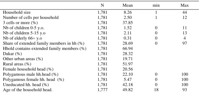
Table 2 describes the main characteristics of Senegalese households. These households are large, with about eight members on average in the PSF sample, with a dependency ratio nearly equal to 50%. They are typically multigenerational and extended both horizontally and vertically, with 28.7% of household members that are neither the head, nor one of his wives or children. Two thirds of households include such “extended” family members.

Polygamous unions are common, with 23% of married men and 35% of married women engaged in such unions. Most of these comprise a husband and two wives (only 20% of polygamous unions have more than two wives). We find that 31% of polygamous men have non-cohabiting wives. In half of these cases, the husband is either considered the head of both households, or of one, while one of the wives is considered head of the other household. In the other half, a married polygamous woman lives in a separate household headed by a relative (mainly her father, brother or son).

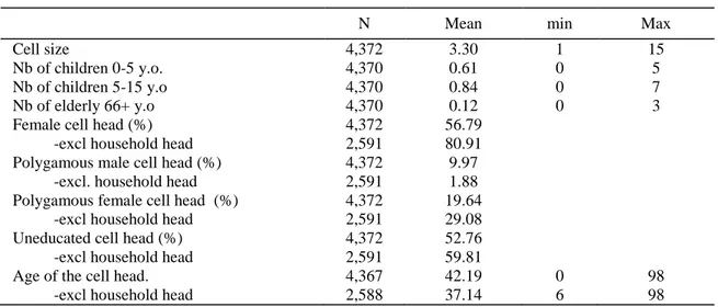
More than half of the households live in rural areas, while 28% are in Dakar. About one fifth of those households are headed by a woman and 40% by an uneducated person. Cells other than the household head’s cell are in vast majority (80%) headed by a woman, who on average are younger and less often educated. Less than 2% of those cells are that of polygamous men that are not household heads.

Table 2a: Household characteristics

N Mean min Max

Household size 1,781 8.26 1 44

Number of cells per household 1,781 2.50 1 12

3 cells or more (%) 1,781 37.85

Nb of children 0-5 y.o. 1,781 1.52 0 11

Nb of children 5-15 y.o 1,781 2.11 0 13

Nb of elderly 66+ y.o 1,781 0.31 0 4

Share of extended family members in hh (%) 1,781 28.69 0 97 Hhold contains extended family members (%) 1,781 66.94

Dakar (%) 1,781 28.32

Other urban areas (%) 1,781 19.71

Rural areas (%) 1,781 51.97

Female household head (%) 1,781 20.56

Polygamous male hh.head (%) 1,781 22.10 0 100

Polygamous female hh. head (%) 1,781 5.47 0 100

Uneducated hh. head (%) 1,781 42.18 0 100

Age of the household head. 1,777 49.82 18 93

8

Table 2b: Cell characteristics

N Mean min Max

Cell size 4,372 3.30 1 15

Nb of children 0-5 y.o. 4,370 0.61 0 5

Nb of children 5-15 y.o 4,370 0.84 0 7

Nb of elderly 66+ y.o 4,370 0.12 0 3

Female cell head (%) 4,372 56.79

-excl household head 2,591 80.91 Polygamous male cell head (%) 4,372 9.97 -excl. household head 2,591 1.88 Polygamous female cell head (%) 4,372 19.64 -excl household head 2,591 29.08 Uneducated cell head (%) 4,372 52.76 -excl household head 2,591 59.81

Age of the cell head. 4,367 42.19 0 98

-excl household head 2,588 37.14 6 98

Source: PSF2006/2007 survey, using sampling weights.

3. I

NEQUALITY AND

I

NTRA

-H

OUSEHOLD

I

NEQUALITIES

LEVELS

a. G

I

.

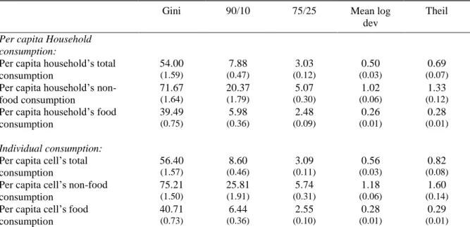
Using per capita household’s expenditures the Gini index is 54 %, quite a bit higher than the one reported in the WDI (40.3% for 2011)7. This difference should be related to the fact that, relative to when it is collected at the household level, collecting consumption data at the cell level leads to an upward revaluation of household consumption that is higher for households that have several income earners or transfer recipients and/or several budgetary units (see section 2.a.). As this is often not the case at the bottom of the distribution, our data reveal that the consumption distribution is more spread out in its upper part than what appears in standard consumption data. This is likely to explain in part why the high level of inequality is not visible when using usual consumption surveys.

As expected, the Gini index of inequality in the distribution of individual food expenditures is much lower than that of non-food spending, reaching 39% vs. 72% (see table 3

7 _{It is slightly lower when using per adult equivalent measure of consumption. See table A1 in the}

9

Table 3: Inequality measures

Gini 90/10 75/25 Mean log dev

Theil

Per capita Household consumption:

Per capita household’s total consumption

54.00 7.88 3.03 0.50 0.69

(1.59) (0.47) (0.12) (0.03) (0.07)

Per capita household’s non-food consumption

71.67 20.37 5.07 1.02 1.33

(1.64) (1.79) (0.30) (0.06) (0.12)

Per capita household’s food consumption

39.49 5.98 2.48 0.26 0.28

(0.75) (0.36) (0.09) (0.01) (0.01)

Individual consumption:

Per capita cell’s total consumption

56.40 8.60 3.09 0.56 0.82

(1.57) (0.46) (0.11) (0.03) (0.08)

Per capita cell’s non-food consumption

75.21 25.81 5.74 1.18 1.60

(1.50) (1.91) (0.31) (0.06) (0.14)

Per capita cell’s food consumption

40.71 6.44 2.55 0.28 0.29

(0.73) (0.36) (0.10) (0.01) (0.01)

Source: PSF2006/2007, N=1728, authors’ calculation, using sampling weights. Bootstrap standard errors (250 replications) between parentheses.

All measures of inequality display the same result: when using the per capita cell’s consumption measure, rather than the per capita household’s consumption, inequality levels are revised upward. Most of the difference comes from the inequality of non-food consumption, while inequality in food consumption is only mildly affected.The Gini of total consumption increases to 56% when each individual is attributed their cell’s per capita consumption level (and that of non-food consumption to 75%).

b. W

.

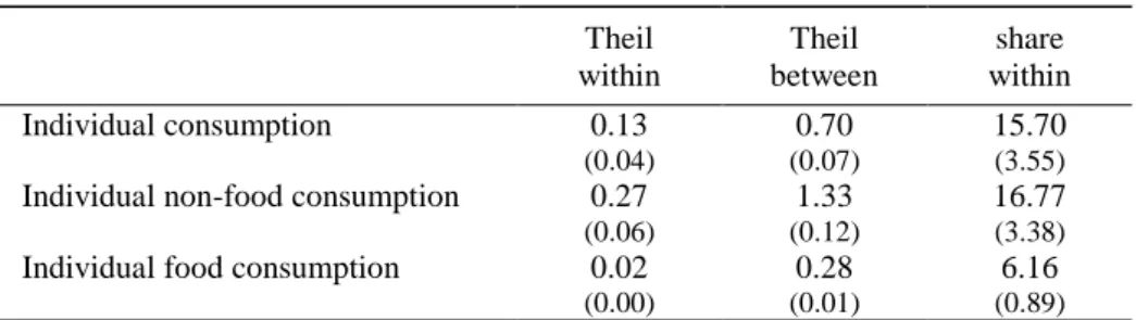
The difference between results based on per capita household’s expenditures and per capita cell’s expenditures might seem small, but it would be wrong to interpret this as the sign of negligible intra-household inequalities. In fact, a Theil decomposition indicates that nearly 17% of total inequalities in non-food expenditures occur within households (table 4). This is obviously much less in the case of food expenditures, reaching only about 6% of total inequalities.

Assuming equal sharing of food between household members eating together possibly underestimates actual intra-household inequality in food consumption. In fact; as household members who partake in the meal share a unique dish, it is hardly possible to measure individual intakes. There are some indications in the literature that in African contexts there exist within households inequalities in the access to nutritional inputs, as testified by the findings of Dercon and Krishnan (2000) or Brown, Ravallion and van de Walle (2017).

10

Table 4: Inequality decomposition

Theil within Theil between share within Individual consumption 0.13 0.70 15.70 (0.04) (0.07) (3.55)

Individual non-food consumption 0.27 1.33 16.77

(0.06) (0.12) (3.38)

Individual food consumption 0.02 0.28 6.16

(0.00) (0.01) (0.89)

Source: PSF2006/2007, N=1728, authors’ calculations, using sampling weights. . Bootstrap standard errors (250 replications) between parentheses

For total consumption, the share of within-households inequality is about 16% of total inequality. Whether this is a large share or not is difficult to assess without a comparison point. We can think of one external comparison, that given by Klasen and Lahori (2016) where they estimate intra-household inequality to be about 30% of total inequality in India. This comparison is interesting but not conclusive for two reasons. First, they base their analysis not on consumption levels but on multidimensional poverty indices, so that the comparison cannot be done directly. It is well known that inequality estimates depend vastly on the variable used for measuring well-being, income inequality being in general much higher than consumption inequality for example. According to the way intra-household allocation of consumption relates to the distribution of endowments, consumption inequality might underestimate more or less seriously inequality in non-monetary outcomes. Second, Klasen and Lahori estimates refer to India, a country that has an income per capita that is much greater than Senegal (1750US$ vs. 1042US$, in 2010 constant dollars, according to the World Bank Indicators), leaving a larger margin for non-subsistence consumption expenditures that are likely to be more unequally shared than those expenditures dedicated to subsistence needs.

Starting from this latter intuition, it is possible to construct from our data a counterfactual situation that maximizes intra-household inequality. In order to do this, we simulated a distribution where everyone gets his observed share of food consumption and of consumption common to the household (such as electricity, water, furniture…). Note that this shared consumption amounts to 69% of total consumption on average. We then attribute all the remaining consumption to the cell of the household head. When doing this, the Theil index of this distribution reaches 93.6 and the within-household Theil index amounts to 24.2. The share of within–household inequality is therefore 25.8% of total consumption inequality. Gauging our result by this counterfactual situation, it seems that the observed within-household inequality is very significant.

Next, we need to assess the robustness of our results to different ways to account for household composition and to possible measurement errors.

Individual consumption can be measured per capita or per adult equivalent. The use of per capita consumption to assess the extent of inequality is likely to yield a higher level of inequality than the use of per adult equivalent consumption if there is a positive correlation between the risk of poverty and the number of children in a household. This is true between households, and also within households and between cells if poor cells have more children than non-poor ones. Hence, using an equivalence scale may provide a different picture on inequality. In appendix table A1 we compute the same inequality measures as those presented in table 3, this time based on consumption per adult equivalent, where a weight of 1 is given to adults, and children between 0 and 14 are weighted 0.5. As can be seen from this table, the difference with per capita estimates is in line with what was expected: inequality based on per adult equivalent consumption is indeed found lower. But the difference is not very high,

11

and the gap between household’s and cell’s consumption estimates remains of the same order of magnitude as that of table 3. As for intra household inequality, appendix table A2 shows the inequality decomposition obtained when using per adult equivalent consumption with two different equivalence scales: scale A is the same as that employed in table A1 while scale B puts a reduced weight on very young children (0.2 for children less than age 4). As can be seen, results are not impacted by the reduced weight given to children: intra-household inequality still accounts for about 16% of the total. So as to ensure that the results are not driven by education expenditures, an important children specific spending unevenly distributed in the population, we replicate the exercise on consumption aggregates net of education expenditures (school fees, furniture and transportation). Results are shown in the bottom part of appendix table A2. As can be seen they are not significantly changed.

Another worry concerning our results is linked to possible measurement errors to which inequality measures are particularly sensitive. In this particular case, because consumption data is collected at the cell level, measurement error will take place at the cell level. In such a case, working at the household level would contribute to average out some of this noise while it would be maximal when working at the cell level. That would suffice to induce some intra-household inequality even if the true distribution is egalitarian. In order to evaluate the sensitivity of our estimates of inequality to such measurement error at the cell level, we will here again resort to simulations. Assuming measurement error takes the form of a white noise, the idea is to assess how large it should be to explain whole of the observed share of intra-household inequality.

The exercise is the following. Assume that the true distribution of consumption is such that there is no intra-household inequality. Everyone in household ℎ gets Yh. Nevertheless, because of (classical)

measurement errors at the cell level, we observe Y_ch which differs from Y_h by a multiplicative random term. Assuming that consumption is log-normally distributed and taking logs, we get:

lnY_ch = lnY_h + u_c

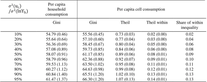
We simulate the observed distributions of Y_ch , varying the magnitude of the error term u_c. This error term is drawn in a normal distribution with a variance fixed at a certain percentage of the variance of the original distribution of log-consumption. This percentage will vary from 10 to 95%. From this new cell consumption data, we compute the equivalent of our two measures of individual consumption: on the one hand we aggregate at the household level to obtain the per capita household consumption; on the other, we construct the per capita cell consumption. We then compute the Gini and Theil indices of the 2 distributions and assess the variance of the white noise that would be enough to explain a level of intra-household inequality equal to 15.7% of total inequality. We replicate simulation 100 times to compute the standard errors of the indices. We will not focus on total level of inequality as the addition of such white noise will mechanically increase it.

Table 5 below gives the result of these simulations. It appears that even with a variance for the error term fixed at 95% of the variance of the original distribution of log-consumption, the decomposition of the Theil index only indicates a within-household share of total inequality of 13%. At 40%, the Gini index for the distribution of per capita cell consumption is 4.6% higher than the one for the per capita household consumption, as we actually observe in our data (4.5%). In both cases, such level of measurement error seems very large so that we are confident measurement error is not the only force driving our results.

The analysis below will confirm that this within-household inequality is not pure noise, as it correlates with a number of observable characteristics of the households.

12

Table 5: Simulated inequality measures in the presence of measurement error

𝜎2_(u c) /𝜎2_(lnY h) Per capita household consumption

Per capita cell consumption

Gini Gini Theil Theil within Share of within inequality 10% 54.79 (0.46) 55.56 (0.45) 0.73 (0.03) 0.02 (0.00) 0.02 20% 55.64 (0.64) 57.10 (0.60) 0.77 (0.04) 0.03 (0.00) 0.04 30% 56.36 (0.69) 58.45 (0.67) 0.80 (0.04) 0.05 (0.00) 0.06 40% 57.08 (0.89) 59.73 (0.85) 0.84 (0.06) 0.06 (0.00) 0.08 50% 58.07 (0.91) 61.17 (0.85) 0.89 (0.06) 0.08 (0.01) 0.09 60% 58.79 (0.96) 62.36 (0.88) 0.92 (0.07) 0.09 (0.01) 0.10 70% 59.53 (1.13) 63.50 (1.02) 0.95 (0.08) 0.11 (0.01) 0.11 80% 60.27 (1.12) 64.63 (0.98) 0.99 (0.08) 0.12 (0.01) 0.12 90% 60.84 (1.40) 65.51 (1.20) 1.02 (0.10) 0.13 (0.01) 0.13 95% 61.47 (1.37) 66.30 (1.20) 1.07 (0.13) 0.14 (0.01) 0.13

Source: authors’ simulated distributions, 100 replications, standard errors between brackets.

c. T

One might want to characterize the level of inequality a given household is experiencing. This can be done in various ways. Table 4 gives the measures of within household Theil indexes and points at a rather high inequality level in terms of non-food consumption. We can also use the ratio of expenditures of the richest cell to that of the poorest. Inequalities within the household are also evident by this measure: the ratio between the expenditures of the richest and poorest cells within a household can be as high as 5.3 after trimming off the 5% most unequal households. On average, the richest cell has a consumption that is more than twice as much as that of the poorest (Table 6).

Using this ratio, it can be seen that it is lower than 1.25 for a good third of the households with 2 cells of more, but greater than 2 for more than a quarter of those households. We will categorize the first group of households as “low inequality” households, the latter as “very high inequality” households, and the remaining middle group as “high inequality” households.

Table 6: Within Household Inequality

N Mean p25 p50 p75

Max/min 1,399 2.42 1.15 1.43 2.08

Low inequality: Max/min<=1.25 1,399 0.36 Very high inequality: Max/min>=2 1,399 0.27

Source: PSF2006/2007, sample of households with 2 cells or more, authors’ calculations.

It is worth noting that in the large households (those with 3 cells or more), the cell of the household head is often the richest cell. One could worry that this is in part spurious if the household head declared as his expenditures some that in fact benefit to the whole household. Nevertheless, the levels of inequality among the other cells of the household are quite high as well, since, excluding the cell of the household head, the ratio of max consumption to min consumption still reaches 2.2 on average. Clearly, in those households with 3 cells or more, within household inequality is higher if we take the head into account (the max to min ratio reaches 3 on average).

13

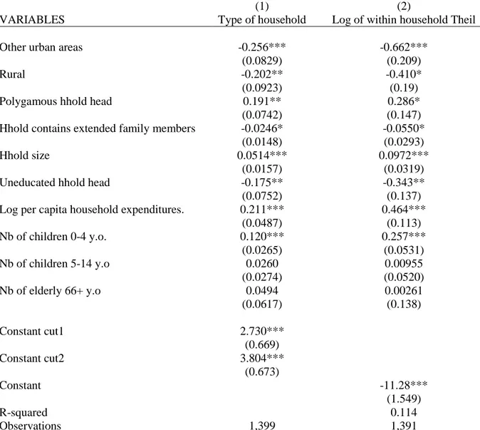
We examine the correlates of being an unequal household (table 7). Column (1) presents the coefficients of an ordered probit estimation for an ordered variable taking value 1 if the household presents a low inequality level, 2 a high inequality level and 3 for a very high inequality level, as defined above. Column (2) gives the OLS estimation where the dependent variable is the log of the within household Theil index. Both approaches give rather similar results.

Household structure clearly plays a role in explaining intra-household inequality. In a nearly mechanical way, larger households are more likely to be unequal. Polygamous households and households with young children appear to also allow for more heterogeneity of consumption levels. In a less expected manner, households containing extended family members display lower levels of inequality. It appears that within household inequality increases with household consumption, and in a related way is lower when the household head is uneducated and higher if the household lives in Dakar.

Table 7: Correlates of within household inequality.

(1) (2)

VARIABLES Type of household Log of within household Theil

Other urban areas -0.256*** -0.662***

(0.0829) (0.209)

Rural -0.202** -0.410*

(0.0923) (0.19)

Polygamous hhold head 0.191** 0.286*

(0.0742) (0.147)

Hhold contains extended family members -0.0246* -0.0550*

(0.0148) (0.0293)

Hhold size 0.0514*** 0.0972***

(0.0157) (0.0319)

Uneducated hhold head -0.175** -0.343**

(0.0752) (0.137)

Log per capita household expenditures. 0.211*** 0.464***

(0.0487) (0.113) Nb of children 0-4 y.o. 0.120*** 0.257*** (0.0265) (0.0531) Nb of children 5-14 y.o 0.0260 0.00955 (0.0274) (0.0520) Nb of elderly 66+ y.o 0.0494 0.00261 (0.0617) (0.138) Constant cut1 2.730*** (0.669) Constant cut2 3.804*** (0.673) Constant -11.28*** (1.549) R-squared 0.114 Observations 1,399 1,391

Source: PSF 2006/2007, authors’ calculations.

(1) Ordered probit estimates : The type of household varies from 1 to 3, 1 being the most equal and 3 the most unequal. (2): OLS estimates.

Additional controls: ethnic group of the household head and religion. Standard errors in parentheses, *** p<0.01, ** p<0.05, * p<0.1

14

The evidence of strong within-household inequality raises the suspicion that some poor individuals might go unnoticed because they live in households where not everyone is poor and that may not be identified as poor by poverty measures based on standard assessments of consumption levels. This issue is explored in the next section.

4. M

EASURES OF POVERTY IN

S

ENEGAL

a. P

In this section we examine the poverty rates obtained from consumption observed at the cell and household levels in the PSF. In order to compare with the results of previous surveys, we choose to use the same poverty lines as that of Ndoye et al. (2009), which presents a poverty profile established with data from the Enquête Suivi de la Pauvreté au Sénégal (ESPS), conducted in Senegal between December 2005 and April 2006. Two lines are retained, established following the basic needs approach. First a food poverty line is defined as the cost of the food basket that provides with at least 2400 kcal per day. The second line is the national poverty line in Senegal. It is obtained by augmenting the food poverty threshold with the amount of resources that is necessary to cover individual basic needs other than nutrition. This amount is obtained through the observation of the average non food consumption of households of which food consumption per adult equivalent is more or less than 5% of the food poverty threshold.

In order to transpose this procedure to our data, we have to hold account of the fact that between 2005-2006 and 2005-2006-2007 when the PSF was on the field, the consumption price index increased. The PSF has been conducted between November 2006 and April 2007, almost exactly a year after the ESPS. In order to estimate the average evolution of the price index between these two periods, we computed the average of the annual inflation rates calculated over the 6 twelve months periods going from November 2005 to November 2006, December 2005 to December 2006, January 2006 to January 2007, February 2006 to February 2007, March 2006 to March 2007 and April 2006 to April 2007. For total consumption this leads to an average one year inflation rate of 4.7% and 5% for food consumption. Table 8 shows the values of the two poverty lines for Dakar, other towns and rural areas separately.

The food poverty line is very close to the $1.25 (PPP 2005) international line (that would be equal to 366 CFA francs at the time of our survey). The $2 line corresponds to 586 CFA francs.

Table 8: Value of the poverty thresholds

Food poverty line National poverty line

Dakar 397 968

Other Towns 370 693

Rural Areas 357 588

15

b. P

,

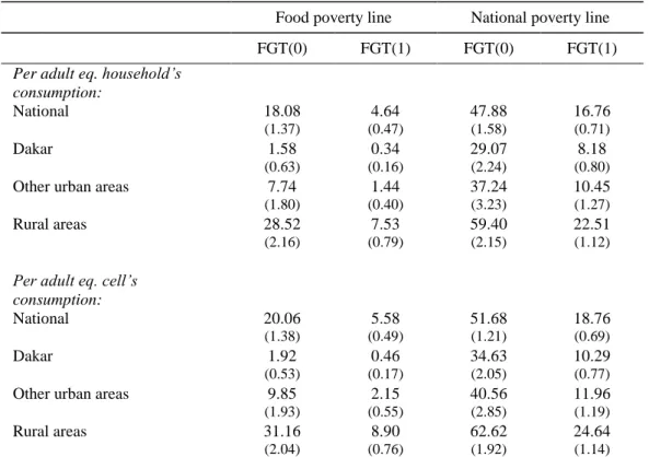
In table 9, we present the various poverty estimates obtained for the two poverty lines. The upper part shows poverty estimates based on per adult equivalent household consumption, while the bottom part present results based on per adult equivalent cell consumption. As already mentioned the overall poverty estimates using PSF are slightly below the measures obtained with the usual consumption survey conducted by the Senegalese statistical office (see table 2). Nevertheless, looking at the upper part, we can see that poverty remains high in Senegal, particularly in the rural areas where it strikes 59% of the population. Acute poverty, measured with the food poverty threshold, is concentrated in the rural areas, where it reaches alarming levels with a bit more than 28% of the population. These results are in line with those obtained by the 2005 Demographic and Health Survey (Ndiaye and Ayad, 2006), which finds that in rural areas 20.6% of children have a height for age z-score below the median WHO reference by more than two standard deviations. This percentage equals 8.5% in urban areas. The same survey shows that 76.8% of children and 54.4% of mothers in urban areas, 85.7% of children and 63.9% of mothers in rural areas were afflicted by a more or less severe form of anaemia. Thus in spite of real progress in the fight against poverty, malnutrition remains an important problem in Senegal.

Table 9: Poverty estimates PSF 2006/2007 - different poverty lines

Food poverty line National poverty line FGT(0) FGT(1) FGT(0) FGT(1)

Per adult eq. household’s consumption:

National 18.08 4.64 47.88 16.76

(1.37) (0.47) (1.58) (0.71)

Dakar 1.58 0.34 29.07 8.18

(0.63) (0.16) (2.24) (0.80)

Other urban areas 7.74 1.44 37.24 10.45

(1.80) (0.40) (3.23) (1.27)

Rural areas 28.52 7.53 59.40 22.51

(2.16) (0.79) (2.15) (1.12)

Per adult eq. cell’s consumption:

National 20.06 5.58 51.68 18.76

(1.38) (0.49) (1.21) (0.69)

Dakar 1.92 0.46 34.63 10.29

(0.53) (0.17) (2.05) (0.77)

Other urban areas 9.85 2.15 40.56 11.96

(1.93) (0.55) (2.85) (1.19)

Rural areas 31.16 8.90 62.62 24.64

(2.04) (0.76) (1.92) (1.14)

Source: PSF2006/2007, authors’ calculations, using sampling weights. Sample sizes are 1728 households and 4206 cells. Bootstrap standard errors (250 replications) between parentheses. Equivalent scale: 0.5: children 0 to 14 years old ; 1: adults.

Strikingly, using per adult equivalent cell consumption rather than per adult equivalent household consumption leads to revise poverty levels upwards, both for the head count and the poverty gap.

16

The results show that the household level approach leads to an underestimation of poverty rates by 0.3 to 5.5 percentage points, depending on the poverty line and the residential area. This corresponds to an underestimation of the prevalence of poverty by 7.3% (national poverty line) and 10.4% (food poverty line) at the national level. The underestimation is particularly severe in Dakar (above 15%), as could have been expected given the especially high within household inequality in that area.

As can be seen in table 9, the difference in poverty measures based on per capita household consumption or per adult equivalent cell consumption depends on the chosen poverty line. The sensitivity of these results to this choice requires further assessment of the robustness of the above findings. Figures 1 to 4 below show the estimated difference between the poverty rates obtained with per capita household consumption and per capita cell consumption depending on the position of the poverty line.8 Figure 1 to 3 show the results obtained for Dakar, the other towns and the rural areas respectively, while figure 4 show those for Senegal as a whole. As we can see the difference between poverty rates is significant for a large range of poverty lines. For rural areas the maximum gap is obtained for a poverty line that lays between the food and national poverty thresholds. For Dakar and other towns, the graph shows that a larger gap would be obtained with higher poverty thresholds, and that below the food poverty lines, the difference is hardly statistically significant.

Figure 1

8 _{Graphs have been drawn using Stata command cfgts2d from the DASP Package and available on line at}

http:// http://dasp.ecn.ulaval.ca/ (Araar and Duclos, 2007).

Food poverty line

National poverty line

-. 0 5 0 .0 5 .1

Value of the poverty threshold

Confidence interval (95 %) Estimated difference

Dakar

17 Figure 2

Figure 3

Food poverty line

National poverty line

-. 0 2 0 .0 2 .0 4 .0 6 .0 8

Value of the poverty threshold

Confidence interval (95 %) Estimated difference

Other urban areas

Difference between poverty rates as a function of the poverty threshold

National poverty line

Food poverty line

-. 0 2 0 .0 2 .0 4 .0 6 .0 8

Value of the poverty threshold

Confidence interval (95 %) Estimated difference

Rural areas

18 Figure 4

c. B

-

.

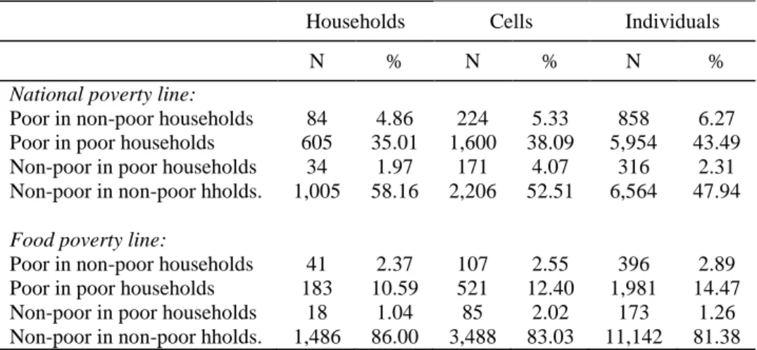
The inequalities documented above induce the existence of poor cells within non-poor households and, inversely, non-poor cells within poor households. This can be seen in table 10, where one finds the distribution of cells according to their poverty status and that of their household. We observe that the proportion of poor cells belonging to a non-poor household varies between 2.6% and 5.3% of cells depending on the poverty threshold (4th column). Looking now at the population percentages (6th column) we observe that poor cells in non-poor households represent a higher proportion of the population than that of cells. The opposite is true for non-poor cells within poor households. In other words poor cells in non-poor households seem to be large cells, and that explains the higher poverty rate when using per adult equivalent cell rather than household consumption.

In total, following the national poverty threshold, about 8%9 of non-poor households include at least one poor cell, which means that 11.6% of the members of non-poor households are in fact poor, or that 12.6% of the poor live in non-poor households. This suggests that measuring poverty using a well-being measure computed at the household level can lead to a serious underestimation of the extent of poverty. 9 _{4.86/(58.16+4.86) from column 2.} -. 0 2 0 .0 2 .0 4 .0 6

Value of the poverty threshold

Confidence interval (95 %) Estimated difference

Senegal

19

Table 10: Distribution of the poor by Poverty Status of their household

Households Cells Individuals

N % N % N %

National poverty line:

Poor in non-poor households 84 4.86 224 5.33 858 6.27 Poor in poor households 605 35.01 1,600 38.09 5,954 43.49 Non-poor in poor households 34 1.97 171 4.07 316 2.31 Non-poor in non-poor hholds. 1,005 58.16 2,206 52.51 6,564 47.94

Food poverty line:

Poor in non-poor households 41 2.37 107 2.55 396 2.89 Poor in poor households 183 10.59 521 12.40 1,981 14.47 Non-poor in poor households 18 1.04 85 2.02 173 1.26 Non-poor in non-poor hholds. 1,486 86.00 3,488 83.03 11,142 81.38

Source: PSF2006/2007, authors’ calculations. Poverty status based on per adult equivalent consumption. Equivalent scale: 0.5: children 0 to 14 years old ; 1: adults.

d. C

H

In this section, we estimate the probability for a household and for a cell to be classified as poor using a logit model. We here define poverty using the national poverty line.

In table 11, column (1) gives the results of the estimation at the household level. Clearly, rural households are more likely to be poor, and this is by far the stronger correlate of poverty, with a risk of poverty more than 2.5 times higher for rural households than for Dakar ones.

Female headed household on the contrary are less often poor. Although this might seem counterintuitive, this finding is relatively general as discussed in van de Walle (2013). It hides massive heterogeneity between these households according to the marital status of the woman (married, widowed or divorced). Non cohabiting married woman and divorcee that head a household are likely to be non-poor, this living arrangement being a choice that can only be made by women who can afford it. As expected, household with a literate head are also less poor.

Of interest to our main point, household structure matters a great deal. In fact, bigger households with a higher dependency ratio tend to be more often poor. But at the same time, for a given household size, having more cells reduces the risk of poverty, by about 30% for each additional cell. This might be due to the fact that an additional cell induces an additional potential income earner.

The second column does the same exercise at the level of the cell. Interestingly, the characteristics of the household head seem to matter as much as that of the head of the cell herself. The cells that are headed by the wife of the household head (the reference category of relations to the household head in the table) are less likely to be poor than any more remote cells.

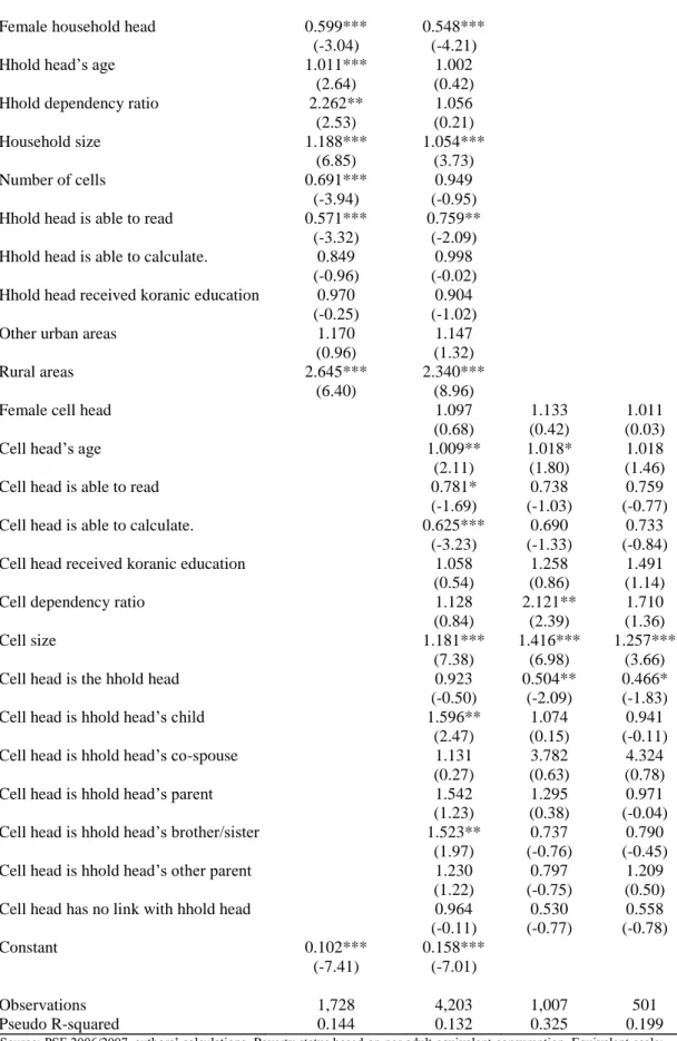
The last two columns of table 11 present the results of a conditional logit estimation that allows removing household fixed-effects. It therefore indicates which characteristics of a cell are correlated with the probability of that cell being among the poor cells in a household where not all cells are poor (and in column 4 where the household as a whole is not poor). It confirms that the cell of the household’s head is the least likely to be poor and that larger cells incur increased risks of poverty.

20

Table 11: Poor Households and poor cells

(1) (2) (3) (4)

VARIABLES Household poverty Cell poverty Cell poverty Cell poverty Hhold FE Hhold FE

Female household head 0.599*** 0.548*** (-3.04) (-4.21)

Hhold head’s age 1.011*** 1.002

(2.64) (0.42) Hhold dependency ratio 2.262** 1.056 (2.53) (0.21)

Household size 1.188*** 1.054***

(6.85) (3.73)

Number of cells 0.691*** 0.949

(-3.94) (-0.95) Hhold head is able to read 0.571*** 0.759**

(-3.32) (-2.09) Hhold head is able to calculate. 0.849 0.998

(-0.96) (-0.02) Hhold head received koranic education 0.970 0.904

(-0.25) (-1.02)

Other urban areas 1.170 1.147

(0.96) (1.32)

Rural areas 2.645*** 2.340***

(6.40) (8.96)

Female cell head 1.097 1.133 1.011

(0.68) (0.42) (0.03)

Cell head’s age 1.009** 1.018* 1.018

(2.11) (1.80) (1.46)

Cell head is able to read 0.781* 0.738 0.759

(-1.69) (-1.03) (-0.77) Cell head is able to calculate. 0.625*** 0.690 0.733

(-3.23) (-1.33) (-0.84) Cell head received koranic education 1.058 1.258 1.491

(0.54) (0.86) (1.14)

Cell dependency ratio 1.128 2.121** 1.710

(0.84) (2.39) (1.36)

Cell size 1.181*** 1.416*** 1.257***

(7.38) (6.98) (3.66) Cell head is the hhold head 0.923 0.504** 0.466*

(-0.50) (-2.09) (-1.83) Cell head is hhold head’s child 1.596** 1.074 0.941

(2.47) (0.15) (-0.11) Cell head is hhold head’s co-spouse 1.131 3.782 4.324

(0.27) (0.63) (0.78) Cell head is hhold head’s parent 1.542 1.295 0.971 (1.23) (0.38) (-0.04) Cell head is hhold head’s brother/sister 1.523** 0.737 0.790

(1.97) (-0.76) (-0.45) Cell head is hhold head’s other parent 1.230 0.797 1.209

(1.22) (-0.75) (0.50) Cell head has no link with hhold head 0.964 0.530 0.558 (-0.11) (-0.77) (-0.78)

Constant 0.102*** 0.158***

(-7.41) (-7.01)

Observations 1,728 4,203 1,007 501

Pseudo R-squared 0.144 0.132 0.325 0.199

Source: PSF 2006/2007, authors’ calculations. Poverty status based on per adult equivalent consumption. Equivalent scale: 0.5: children 0 to 14 years old ; 1: adults. (a) Observation unit: household, column (1); cell, columns (2), (3) and (4). (b) Estimated model: logit, columns (1) and (2); conditional logit (household fixed effects), columns (3) and (4). In column (3) all cells belonging to households in which some cells are poor but not all are included, no matter if the household is poor or not. In column (4), only cells belonging to non-poor households are included. (c) Reference category for relation of the cell head to household head: Cell head is the wife. (d) Odds ratios are presented. Robust z-statistics in parentheses *** p<0.01, ** p<0.05, * p<0.10.

21

e. A

-

POOR

?

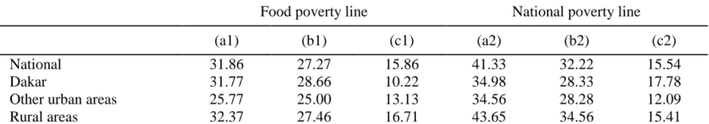
How poor are the poor that live in non-poor households? A natural question is that of whether the intensity of poverty is lower for them than for those who live in households where everyone is poor. Table 12 gives some elements to answer this question by presenting the poverty gap for the poor who live in non-poor households (columns c1 and c2) and comparing it to that of the poor from homogeneously poor households (a1 and a2), and from poor households with non-poor members (b1 and b2).

Table 12: Poverty gaps for poor cells in poor and non-poor households

Food poverty line National poverty line

(a1) (b1) (c1) (a2) (b2) (c2)

National 31.86 27.27 15.86 41.33 32.22 15.54

Dakar 31.77 28.66 10.22 34.98 28.33 17.78

Other urban areas 25.77 25.00 13.13 34.56 28.28 12.09

Rural areas 32.37 27.46 16.71 43.65 34.56 15.41

Source: PSF2007/2007, authors’ calculations. Poverty status based on per adult equivalent consumption. Equivalent scale: 0.5: children 0 to 14 years old ; 1: adults. Columns (a1) and (a2) show the value of the poverty gap for poor cells in poor households in which all cells are found poor; columns (b1) and (b2) show the value of the poverty gap for poor cells in poor households, in which some cells are found not poor and columns (c1) and (c2) show the value of the poverty gap for poor cells in non-poor households.

Table 12 shows quite clearly that the poor in non-poor households are less poor than other poor. At the national level, the poverty gap for this group is only half that of the poor who live in poor households that contain non-poor members. It reaches only 37% of the poverty gap of the poor in poor households. This is understandable as within household inequality is more likely to push part of the household members on the other side of the poverty line if the household as a whole is not too far from it. It suggests that the “invisible poor” are likely to be among the least poor of the poor.

5. C

ONCLUSION

This paper uses a novel survey to reveal the extent of both total inequality and within household consumption inequalities. We show that global inequality is much higher than what was previously thought, with a Gini coefficient reaching nearly 54 while international statistical yearbooks give a Gini of 40. Within-household inequality accounts for nearly 16% of total inequality in Senegal. One of the consequences of such unequal repartition of resources within households is the potential existence of “invisible poor” in households classified as non-poor. Our assessment is that as many as 12.5% of the poor individuals live in non-poor households. They are therefore ignored when the poverty status of the household is supposed to apply uniformly to all household members. This could have important consequences for the effectiveness of anti-poverty policies.

To uncover these facts, we innovated by designing a consumption survey that collects information at the level of sub-groups within the household, using different respondents for different cells. This allowed us collecting more complete consumption data, so that total consumption is measured to be

22

higher than what was obtained with a classical consumption survey at the same period. More central to this paper, this approach permitted to measure consumption at a relatively individualized level and thereby to exhibit the within household unequal access to consumption.

When households are large and of a complex structure, as in Senegal and in many sub-Saharan African countries, where several relatively autonomous budgetary units cohabit, it is not the case that everyone has access to the same level of resources. In these contexts, coming as close as possible to the individual when measuring welfare is crucial in order to obtain adequate measures of poverty and help anti-poverty policies to efficiently target the poor.

Our results suggest that the more complex the household structure, the bigger the household size, the more inequality is likely to be underestimated when computed using standard consumption surveys. This would imply that cross-country comparisons of inequality levels should take into account that difference in family structure and organisation will translate into artificial differences in inequality levels.

23

R

EFERENCES

Araar Abdelkrim and Jean-Yves Duclos (2007), "DASP: Distributive Analysis Stata Package", PEP, World Bank, UNDP and Université Laval.

Baland, Jean-Marie, Catherine Guirkinger, and Charlotte Mali (2011),. "Pretending to Be Poor: Borrowing to Escape Forced Solidarity in Cameroon." Economic Development and Cultural

Change 60, no. 1 (2011): 1-16.

Beck, Simon, Philippe De Vreyer, Sylvie Lambert, Karine Marazyan and Abla Safir (2015), « Child fostering in Senegal », The Journal of Comparative Family Studies, vol 46: 57-73

Beegle Kathleen, De Weerdt Joachim, Friedman Jed and John Gibson (2012), “Methods of

household consumption measurement through surveys: Experimental results from Tanzania”,

Journal of Development Economics, Volume 98, Issue 1, May 2012, pp 3-18.

Boltz Marie, Karine Marazyan and Paola Villar (2015), « Preference for Hidden Income and Redistribution to Kin and Neighbors: A Lab-in-the-field Experiment in Senegal”. PSE Working Papers n° 2015-15.

Brown Caitlin, Martin Ravallion and Dominique van de Walle (2017), “Are poor Individuals Mainly Found in Poor households?”, Policy Research Working Paper 8001, World Bank.

Chiappori, Pierre-Andre, (1988). "Rational Household Labor Supply," Econometrica, Econometric Society, vol. 56(1), 63-90, January

Cogneau Denis, Bossuroy Thomas, De Vreyer Philippe, Guenard Charlotte, Hiller Victor, Leite Philippe, Mesple-Somps Sandrine, Pasquier-Doumer Laure, and Constance Torelli (2006), « Inégalités et équité en Afrique », DIAL WP 2006-11.

Dercon, Stefan, and Krishnan Pramila (2000), "In Sickness and in Health: Risk Sharing within Households in Rural Ethiopia." Journal of Political Economy 108, no. 4 (2000): 688-727.

De Vreyer, Philippe, Sylvie Lambert, Momar Sylla and Abla Safir (2008), “ Pauvreté et Structure Familiale. Pourquoi une nouvelle enquête ?”, Statéco, n°102, pp. 5-20.

Dunbar, Geoffrey R., Arthur Lewbel and Krishna Pendakur. (2013),. "Children's Resources in Collective Households: Identification, Estimation, and an Application to Child Poverty in Malawi." American Economic Review, 103(1): 438-71.

Klasen, Stephan and Rahul Lahoti (2016), “How Serious is the Neglect of Intra-Household Inequality in Multi-dimensional Poverty Indices”, CRC-PEG Discussion Papers No. 200.

Lambert, Sylvie and Pauline Rossi, (2016), "Sons as widowhood insurance: Evidence from Senegal" ,Journal of Development Economics, vol. 120: 113-127

Ndiaye, Salif, Mohamed Ayad (2006), "Enquête Démographique et de Santé. Sénégal 2005", Ministère de la Santé et de la Prévention Médicale. Centre de Recherche pour le Développement Humain. Dakar.

24

Ndoye, Djibril, Franck Adoho, Prospère Backiny-Yetna, Mariama Fall, Papa Thiecouta Ndiaye, Quentin Wodon (2009), "Tendance et profil de la pauvreté au Sénégal de 1994 et 2006", MPRA Paper No. 27751.

Rose, Elaina (1999), “Consumption Smoothing and Excess Female Mortality in Rural India”,

Review of Economics and Statistics, 81:1, 41-49

Van de Walle, Dominique (2013), « Lasting Welfare Effects of Widowhood in Mali », World

Development, Volume 51, November 2013, Pages 1–19

Van de Walle, Etienne and Aliou Gaye (2006): “Household structure, polygyny and ethnicity in Senegambia: a comparison of census methodologies”, in Etienne van de Walle, ed. : African

Households : censuses and Surveys. New York, M. E. Sharpe Inc.

World Bank (2015), World Development Report 2016: Equity and Development, World development report. Washington, DC : World Bank Group, Oxford University Press

Ziparo Roberta (2016) : “Why do spouses communicate : Love or interest? A model and some evidence from Cameroon”, mimeo

25

Table A1: Inequality measures, on per adult equivalent consumption.

Gini 90/10 75/25 mean log dev

theil

Per adult equivalent household’s consumption

Per adult equivalent

household’s total consumption

52.02 7.28 2.82 0.46 0.64

(1.66) (0.47) (0.12) (0.03) (0.06)

Per adult equivalent hhold’s non-food consumption

70.40 18.73 4.73 0.97 1.27

(1.72) (1.29) (0.25) (0.06) (0.11)

Per adult equivalent food hhold’s food consumption

37.71 5.47 2.34 0.24 0.25

(0.76) (0.33) (0.08) (0.01) (0.01)

Per adult equivalent cell’s consumption

Per adult equivalent cell’s total consumption

54.01 7.76 2.87 0.51 0.76

(1.62) (0.46) (0.09) (0.03) (0.08)

Per adult equivalent cell’s non-food consumption

73.64 22.82 5.25 1.11 1.52

(1.59) (1.65) (0.24) (0.06) (0.14)

Per adult equivalent cell’s food consumption

38.78 5.91 2.40 0.25 0.27

(0.74) (0.35) (0.08) (0.01) (0.01)

PSF2006/2007, N=1728, authors’ calculation, using sampling weights. Bootstrap standard errors (250 replications) between parentheses. Equivalent scale: 0.5: children 0 to 14 years old ; 1: adults.

Table A2: Inequality decomposition, per adult equivalent consumption

Theil within Theil between Share within Scale A Individual consumption 0.12 0.64 15.82 (0.04) (0.06) (3.94) Individual non-food consumption 0.25 1.27 16.66 (0.07) (0.11) (3.64)

Individual food consumption 0.01 0.25 5.47

(0.00) (0.01) (0.80) Scale B Individual consumption 0.12 0.61 16.34 (0.04) (0.06) (4.27) Individual non-food consumption 0.26 1.24 17.08 (0.08) (0.11) (3.90)

Individual food consumption 0.02 0.25 6.09

(0.00) (0.01) (0.69)

Scale A – without educational expenditure Individual consumption 0.12 0.63 16.39 (0.04) (0.07) (4.04) Individual non-food consumption 0.27 1.29 17.35 (0.07) (0.12) (3.74)

PSF2006/2007, N=1728, authors’ calculation, using sampling weights. Bootstrap standard errors (250 replications) between parentheses. Scale A: 0.5: children 0 to 14; 1: adults ; Scale B: 0.2: children 0 to 4 ; 0.5: children 5 to 14; 1: adults.