WORKING
PAPERS
SES
N. 474
IX.2016
Reversal of Migration Flows:
A Fresh Look at the German
Reunification
Volker Grossmann,
Andreas Schäfer,
Thomas Steger,
Reversal of Migration Flows: A Fresh Look at the
German Reunification
∗
Volker Grossmann
†, Andreas Schäfer
‡, Thomas Steger
§, Benjamin Fuchs
¶September 14, 2016
Abstract
We investigate the dynamic effects of interregional labor market integration on migration flows, capital formation, and the price for housing services. The co-evolution of these variables depends on initial conditions at the time of labor market integration. In an initially capital-poor economy, there may be a reversal of migration flows during the transition to the steady state, while housing costs are increasing over time. Although capital may accumulate while labor emigrates early in the transition, the causal effect of immigration on capital investments and housing costs is positive. We present new data on the evolution of net migration flows and rental rates for housing in East Germany after 1990. Our results are consistent with the presented evidence in the reverse migration scenario.
Key words: Capital formation; German reunification; Housing services; Labor market integration; Reverse migration.
JEL classification: D90, F20, O10.
∗Acknowledgements: We are grateful to seminar participants at Stockholm University, the Univer-sity of Göttingen, the 4th Norface Migration Network Conference on "Migration: Global Development, New Frontiers" in London, the annual meeting of the European Economic Association in Gothenburg, the annual meeting of German-speaking economists ("Verein für Socialpolitik") in Münster, and the World Trade Institute in Bern for helpful comments and suggestions. Jan Bruch, Isabelle Manthey, and Johann Teller provided excellent research assistance.
†University of Fribourg; CESifo, Munich; Institute for the Study of Labor (IZA), Bonn; Centre for Research and Analysis of Migration (CReAM), University College London. Address: University of Fribourg, Department of Economics, Bd. de Pérolles 90, 1700 Fribourg, Switzerland. E-mail: [email protected].
‡ETH Zurich; Leipzig University. Address: ETH Zurich, Zürichbergstr. 18, CH-8092 Zurich, Switzerland. Email: [email protected].
§Corresponding author: Leipzig University; CESifo, Munich, Halle Institute for Economic Re-search (IWH). Address: Institute for Theoretical Economics, Grimmaische Strasse 12, 04109 Leipzig, Germany. Email: [email protected].
¶University of Hohenheim. Address: Department of Economics (520B), 70593 Stuttgart, Germany. Email: [email protected].
“Today, the decision was taken that makes it possible for all citizens to leave the country through East German border crossing points. [...] As far as I know - effective immediately, without delay.”1
1
Introduction
The fall of the Berlin Wall in November of 1989 can be viewed as a quasi-natural experiment of the effects of interregional labor market integration. From one day to the next, literally overnight, East German citizens had the opportunity to move to West Germany (and vice versa), after the sudden removal of all institutional migration barriers. To begin with, there were no language barriers. Moreover, there were plenty of family ties that made migration costs, other than costs associated with finding a new shelter, almost negligible. In other words, we have seen a historically unique case of an exogenous integration shock from fully closed to fully open borders.
This paper examines the dynamic effects of interregional labor market integration on migration patterns, private investment, wages, and the price for housing services. In particular, we take up the challenge to explain the mechanics of the remarkable migra-tion pattern in East Germany for the period 1991-2014. This period is characterized by a “reversal of migration flows”, i.e. prolonged net outward migration followed by net inward migration later on. Fig. 1 shows the net migration flows for East Germany (“New Laender”), excluding Berlin. To smooth out business cycle fluctuations, we take five-year annual averages for the periods 1991-1995, 1996-2000, 2001-2005 and 2006-2010 as well as the four-year annual average for the period 2011-14. According to Fig. 1, there was a massive outflow in the 1990s and 2000s for East Germany as a whole.2
The outflow was larger for the 1990s when leaving out the state of Brandenburg that is special in the following sense. Many workers of Berlin-based firms are commuting
1Guenther Schabowski (First Secretary of the East Berlin chapter of the Socialist Unity Party -SED - in the former German Democractic Republic - GDR - and a member of the -SED Politbuero), November 9, 1989. Translated from German.
2Burda (2006) also documents for the 1990s labor outflows from East Germany that were directed to West Germany.
-50,000 -40,000 -30,000 -20,000 -10,000 0 10,000 20,000 1991 - 1995 1996 - 2000 2001 - 2005 2006 - 2010 2011 - 2014 All W/o Brandenburg
Figure 1: Net migration flows (annual averages) to the New Laender (Brandenburg, Mecklenburg-Western Pomerania, Saxony-Anhalt, Saxony, and Thuringia), 1991-2014. Data: See Online Appendix.
to work from Brandenburg that surrounds the city of Berlin (partly having belonged to West Germany).3 The migration pattern in the New Laender has reversed to net
inflows after 2011. As displayed in Figure 2, the reversal of migration flows is particu-larly apparent for cities with more than 100,000 inhabitants. It has started already in the 2000s, with the largest inflows to the two largest cities, Dresden and Leipzig. More recently there have been positive net inflows to all East German cities.
To explain such a migration pattern, we develop a neoclassical, overlapping gener-ations model with a tradable goods sector and a housing sector. The housing sector combines land and residential structures, that is accumulated through construction ac-tivities, to produce housing services.4 Firms in the tradable goods sector face capital
adjustment costs to install new physical capital. We study the effects of implementing
3Associated with Berlin having become an economic and political center soon after the German reunification, Brandenburg experienced net immigration in the mid 1990s.
4This borrows from the business-cycle literature on housing and macroeconomics (Davis and Heath-cote, 2005; Hornstein, 2008, 2009; and Favilukis et al., 2015). Chambers et al. (2009a, 2009b) employ an OLG model with housing and mortgage markets, excluding the fixed factor land, to explain the evolution in homeownership rates. Grossmann and Steger (2016) develop a long-term macroeconomic model. Piazzesi and Schneider (2016) provide an excellent survey.
-7,000 -6,000 -5,000 -4,000 -3,000 -2,000 -1,000 0 1,000 2,000 3,000 4,000 5,000 6,000 7,000 8,000 9,000 10,000 11,000 1991 - 1995 1996 - 2000 2001 - 2005 2006 - 2010 2011 - 2014 Potsdam Rostock Leipzig Dresden Halle (Saale) Magdeburg Erfurt Jena
Figure 2: Net migration flows (annual averages) to cities with more than 100,000 inhabitants in the New Laender, 1991-2014. Data: See Online Appendix.
free interregional labor movement, conditional on initial differences (across regions) in the two capital stocks (physical capital and residential structures) and on initial differ-ences in productivity levels. These interregional differdiffer-ences drive migration decisions by determining differences in both wage rates and the price for housing services across regions.
Our analysis suggests a causally positive (negative) effect of immigration (emigra-tion) on capital accumulation. Nevertheless, interregional flows of labor and regional changes in capital stocks may transitorily evolve in opposite directions.5 We
demon-strate how initial conditions and the time that has elapsed after labor market inte-gration determine how miinte-gration flows are related to the evolutions of capital stocks and housing costs over time. In particular, we show that in the case of low initial pro-ductivity levels and / or low initial capital stocks, such as in East Germany vis-à-vis
5Historically, there are examples for labor and capital to flow in the same or in opposite directions. For instance, the Atlantic globalization in the 19th century was characterized by simultaneous capital and labor flows from Europe to the US (e.g. O’Rourke and Williamson, 1999; Solimano and Watts, 2005). Moreover, in response to the enlargement of the European Union (EU), labor was migrating from Southern and Eastern EU members to countries like Germany and the UK, while there were net
West Germany at the time of the German reunification, a net outflow of migrants may occur, in an early transition phase, despite accumulation of capital stocks. In later phases, the migration pattern is reversed along with still positive net investments. Net investments in physical capital and structures are indeed positive if the neoclassical convergence force is sufficiently strong or if productivity levels increase over time (e.g. following technology transfers like those from the Old Laender to the New Laender). The price for housing services is increasing as the economy develops, reflecting the scarcity of land and the increase of wage rates over time.
Noteworthy, the suggested model can also explain, under alternative initial condi-tions, other migration patterns, such as continuous immigration or continuous emigra-tion in response to labor market integraemigra-tion. For instance, consistent with our frame-work, there were massive net immigration flows to Switzerland (a high-productivity economy with a high capital-to-labor ratio) along with rising prices for housing ser-vices in the aftermath of the bilateral agreement with the European Union on the free movement of labor.6 We focus on the German case after 1989, however, because
this historical episode was shaped by a unique experiment that allows us to better understand the dynamic general equilibrium mechanics of migration and capital accu-mulation in general and the reverse migration phenomenon in particular.
We also show that higher population density causally raises housing costs even in the long run, i.e. after housing supply fully adjusted to the increase in housing demand as a response to immigration. This finding is consistent with the evidence on causally positive effects of immigration on both the price for housing services and residential construction (e.g. Gonzalez and Ortega, 2013).7 The reason is that the production of
6The agreement was signed in 2002 and came into full effect (with respect to 17 EU countries, excluding Eastern Europe) in 2007. The case of Switzerland is discussed in detail in the working paper version of this paper (Grossmann, Schäfer and Steger, 2013).
7Gonzalez and Ortega (2013) employ Spanish regional data for the period 2001-2010 (characterized by an annual population growth rate of 1.5 percent). They instrument changes in population density by past migration stocks of the foreign-born population in a region. About half of the construction boom in the 2000s is attributed to immigration. Saiz (2003, 2007) and Nygaard (2011) find substantial effects of immigration on rental rates and sales prices for housing in the US and UK. Jeanty et al. (2010) estimate a two-equation spatial econometric model which captures the two-way interaction between net migration flows and the price for housing services. Employing data from the metropolitan area of Michigan, they find that a one percentage point increase in the rate of population growth leads to a
housing services is land-intensive and land is a fixed factor that becomes increasingly scarce in a growing economy. Thus, the price of housing services is closely related to the rental rate of land (Knoll, Schularick and Steger, 2016; Grossmann and Steger, 2016).
The main contribution of the paper is twofold. First, whereas a large literature on the dynamic effects of migration was confined to either the labor market or the housing market separately, we shift the focus to the interaction between housing costs and wage rates over time in determining migration patterns.8 We show that a re-versal of migration patterns can be explained by the interaction between migration, capital investment, and construction activities. Standard neoclassical models cannot explain the reversal of migration flows.9 While our model shares the features of capital
adjustment costs, exogenous interest rates and interregional labor mobility with the one-sector frameworks developed in Rappaport (2005) and Burda (2006), their focus is on wage convergence rather than on the reversal of migration flows.10 We show that the reversal of migration flows is generated by the dynamics of residential construc-tion and the price for housing services that we addiconstruc-tionally examine in our two-sector framework. Moreover, whereas non-monotonic time paths of a region’s population size may occur in models with increasing returns to scale, our framework explains non-monotonic transitions despite constant returns to scale.11 Second, the paper provides a
0.24 percent increase in housing costs.
8Important studies on wage effects of immigration include Friedberg (2001) for Israel, Dustmann, Fabbri, and Preston (2005) for the UK, and Borjas (2003) as well as Ottaviano and Peri (2012) for the US.
9Felbermayr, Grossmann and Kohler (2015) provide an extensive literature survey on the interac-tion between migrainterac-tion and capital formainterac-tion.
10Rappaport (2005) argues that higher labor mobility that leads to an increased outflows of workers does not necessarily increase the speed of income convergence. For a given capital stock, emigration leads to increased wages in the source country. However, emigration also drives down the shadow value of capital and therefore slows down capital investment. The latter effect results in delayed income convergence. Burda (2006) studies the dynamics of labor migration and capital accumulation under factor adjustment costs. Per capita income of the East German economy fully converges to the West German level as labor moves towards West Germany and capital accumulates in the East Germany economy.
11Faini (1996) contrasts models of exogenous and endogenous growth, arguing that income conver-gence is not necessarily less likely in the case of learning-by-doing effects. Reichlin and Rustichini (1998) employ an endogenous growth model with learning-by-doing effects to show that immigration enhances interregional wage differences due to a scale effect, benefitting the receiving destination.
new comprehensive data set for the New Laender in Germany at the regional (county and state) level on net migration flows and on the rental costs of housing services for the period after the German reunification until 2014. It is demonstrated that our results are qualitatively consistent with the presented evidence.
The paper is organized as follows. Section 2 presents the model. Section 3 pro-vides analytical results for the long run equilibrium. In Section 4, we solve the model numerically for the transition path to the steady state in response to labor market integration. We demonstrate the model’s potential to explain a reversal of migration flows and discuss the salient role of the housing sector for this outcome. Section 5 demonstrates that the suggested explanation for the reverse migration phenomenon is also consistent with the joint evolution of housing rental rates and wage rates in East Germany after 1990. The last section concludes.
2
The Model
Consider a simple neoclassical model economy with two sectors. The tradeable goods sector produces a final good (the "numeraire"). The non-tradable goods sector pro-duces housing services by combining accumulable "structures" and a fixed amount of land. Labor can be reallocated across sectors without any frictions. There is interna-tional mobility of physical capital at an (exogenous) interest rate 0. Labor market integration allows individuals to move between two regions ("domestic" and "foreign"). We distinguish the cases of interregionally immobile and mobile labor, investigating the effects of labor market integration. Time is discrete and indexed by = 0 1 2
Moreover, migration may change the skill composition of the workforce in a way which may also bene-fit the source economy. Schäfer and Steger (2014) emphasize how equilibrium selection and dynamics depend on both expectations and initial conditions in a multi-region model where increasing returns give rise to multiple equilibria.
2.1
Domestic Economy
2.1.1 Firms
There is a tradable goods sector producing a homogenous good, which is chosen as numeraire (i.e. output price
≡ 1). The production technology of the representative firm is given by
= ·
¡
¢()1− (1)
∈ (0 1), where denotes the amount of labor, physical capital, and 0
total factor productivity (TFP) in the tradable goods sector.12 Accumulating physical
capital is subject to (convex) capital-adjustment costs (Abel, 1982; Hayashi, 1982). Let denote the amount of the tradable good that is devoted to gross investment in
the tradable goods sector. Taking the time path of the wage rate, , as well as the (exogenous) interest rate, , as given, the representative firm solves
max { }∞=0 ∞ X =0 ·¡ ¢ ()1−− − h 1 + ³ ´i (1 + ) (2) s.t. +1 = + (1− ) , (3)
where 0 is the depreciation rate of physical capital and 0 0 is given.
The non-tradable sector produces residential structures (a non-tradable stock) and housing services (a non-tradable flow). The representative construction firm combines labor, , and materials (e.g. cement), , to manufacture gross investment in
struc-tures, , according to
= ·¡¢()1− (4)
∈ (0 1), where 0 is TFP in the construction sector. Materials are produced from the tradable good on a one-by-one basis. The stock, , depreciates at rate 0 and
accumulates according to +1 = + (1− ) (5) = ·¡ ¢ ()1− + (1− ), (6)
where 0 0 is given. The representative construction firm then solves
max { }∞=0 ∞ X =0 − − (1 + ) s.t. (6), (7)
taking , , and as given. The representative housing services firm produces a non-tradable consumption good by combining structures and a fixed (i.e., time-invariant) amount of land (which equals land supply), according to
= ()1− (8)
∈ (0 1).13 Denote by the price per unit of housing services, by the rental rate per unit of structures, and by the rental rate of land. Each period , the
representative housing services firm solves
max ¡ () 1−− − ¢ (9)
taking , , and as given.
2.1.2 Households
Each individual lives for two periods ("working-age" and "retirement") and has one child when old. In the first period, each individual supplies one unit of labor when young to the sector with the highest wage and chooses how much to save (or borrow). Moreover, individuals decide at the beginning of the first period whether to stay or to migrate to the large economy, seeking to maximize life-time utility. Our simple
13TFP in the housing services sector is set to unity. A higher captures better technology in the housing sector as a whole.
overlapping-generations structure allows us to focus on one-shot migration decisions of workers. There may be (exogenous) institutional and social migration costs, denoted as ∆ ≥ 0. We assume that a worker migrates if and only if the utility gain from migrating is equal to or higher than ∆. As will become apparent, even if ∆ = 0 (no exogenous migration costs) and despite persistent wage differentials, migration flows are limited via differences in the price of housing services across regions. Migration flows are therefore smoothed endogenously along with adjustments in the stocks of physical capital and residential structures.
The number of workers (i.e. the number of young individuals) in period is denoted by . Thus, total population size in period is given by + −1. The number of
initially old natives, −1 0, is given. As each period the same number of individuals is born, = −1 for all ≥ 0 if labor is not interregionally mobile. The population
density is given by ≡ (+ −1), where −1 0is given. Labor market clearing
requires
+ = (10)
Initially land is fully owned by the −1old natives, where () denotes the landhold-ing of individual . Landowners bequeath their landholdlandhold-ing to their child when leavlandhold-ing the scene, such that the number of landowners and the land distribution among natives is time-invariant. For simplicity, we assume that firms in the non-tradable goods sector are owned by foreigners. In period , a young individual who stays in the domestic economy thus has a present discounted value of life-time income, (), which is given
by
() = +
+1
1 + () (11)
For the sake of realism, suppose that a non-negligible fraction of natives is landless (for a landless individual , () = 0).
Let 1and 1denote the amount of tradable goods and housing services consumed
by a working-age individual born in , respectively. Analogously, 2+1 and 2+1 are
is given by14
() = (1() 1()) + · (2+1() 2+1()) (12)
∈ (0 1), with instantaneous utility function ( ) = ·log +(1−)·log , ∈ (0 1). Recalling that = 1, the intertemporal budget constraint of consumer reads as
1() + 1() +
2+1() + +12+1()
1 + ≤ (). (13) We assume that the time discount rate is given by the standard condition
· (1 + ) = 1 (14)
2.2
Foreign Economy
The foreign economy is in steady state and large in the sense that migration from or towards the domestic economy has no effect on its population density. The popula-tion density, denoted by ∗(= ∗∗), is therefore time-invariant. TFP levels in the
tradable goods sector of the foreign economy, ∗, and in the housing sector, ∗, may differ from the domestic levels, and , respectively. Apart from productivity levels, population density, and initial conditions, the domestic and the foreign economy are identical.
3
Equilibrium Analysis
As shown in the appendix, individual has life-time utility
(() +1) ≡ max 1()1()2+1()2+1() () s.t. (13) (15) = Ω + (1 + ) log ()− (1 − ) £ log + log +1 ¤ (16)
14This preference specification can be viewed as a dynamic extension of the static model of locational choice by Roback (1982), who argues that differences in wage income across regions can be explained by different amenities associated with the chosen location, also endogenizing the rental rate of land.
with Ω ≡ (1 + ) log³(1−)1+1−
´
. Let ∗ denote the wage rate and ∗ the price for
housing services in the foreign economy. Moreover, define by V≡ ( +1) and
V∗ ≡ (∗ ∗ ∗) the life-time utility (in equilibrium) of a landless native in the
domestic and foreign economy, respectively. If labor is interregionally mobile, landless domestic residents born in do not want to migrate to the foreign economy as long as V≥ V∗+ ∆. Similarly, landless foreign residents born in do not want to migrate to
the domestic economy as long as V+∆≤ V∗. If ∆ 0, there is the possibility that, for
a given set of parameters, a multiplicity of equilibria = −1 (no migration) exists
whenever |V− V∗| ≤ ∆ (indeterminacy of equilibrium).15 To avoid such difficulty and
to capture the absence of institutional migration costs within Germany after the fall of the Berlin Wall, we follow Roback (1982) and abstract from exogenous migration costs in the remainder of this paper, assuming ∆ = 0. We focus on equilibria where landless individuals are indifferent whether or not to migrate under integrated labor markets, such that
V=V∗ for any ≥ 1 (17)
If ∆ = 0, a domestic native born in with land holding () does not want to migrate to the foreign economy if
(+ · +1() +1) (∗ + · +1() ∗ ∗) (18)
Using (16) in (18), the incentive-compatibility constraint for a domestic native born in with land holding () to remain in the domestic region reads
1 + 1− log µ + · +1· () ∗ + · +1· () ¶ log µ ∗ ¶ + · log µ +1 ∗ ¶ (19)
Notice that for 0, we have +·∗+··· ()
∗ if ()∗. Thus, if ∗
and = ∗ holds, a land-owning domestic native does not want to migrate to the
15Armenter and Ortega (2011) employ a static multi-regions model with skilled and unskilled workers under endogenous redistribution and mobility costs. In their setup, redistribution and mobility costs affect the incentives for skilled workers to migrate. Interestingly, they obtain multiple equilibria if
foreign economy, as the incentive-compatibility constraint (19) is satisfied. In contrast, if ∗ and V = V∗ holds in equilibrium, a land-owning foreign native does not
want to migrate to the domestic economy. In other words, when landless individuals are indifferent in equilibrium whether or not to migrate, triggered off by emigration of some landless individuals motivated by gaining wage income, no landowner wants to migrate.16 The intuition why the incentive to migrate is higher for landless individuals is as follows. Because land rents are received from the home region irrespective of the location decision, income-related migration benefits come from wage differentials only. As the marginal utility from consumption is declining, wage gains from migration matter more for landless individuals.
3.1
Interregionally Immobile Labor
It turns out that, for all , the equilibrium levels of all factor inputs per unit of land, ≡ , ≡ , ≡ , ≡ , ≡ , are independent of total
land supply . Before entering the numerical analysis in Section 4, we characterize the long-run equilibrium analytically. Denote the long-run equilibrium value before labor market integration of any variable by ˜. All proofs are relegated to the Appendix.
Proposition 1. In an interior long run equilibrium before labor market integration, (i) an increase in population density, , raises factor inputs ˜, ˜, ˜, ˜, ˜, the
price of housing services, ˜, and the rental rate of land, ˜, whereas the wage rate, ˜
, and the price of structures, ˜, do not depend on ;
(ii) an increase in the tradable goods sector’s TFP level, , raises capital inputs ˜, ˜
, as well as the input of materials, ˜, the price of housing services, ˜, the rental
rate of land, ˜, the wage rate, ˜, and the price of structures, ˜, whereas labor inputs ˜
, ˜ remain unaffected;
16Conversely, if landless individuals are indifferent whether or not to migrate although wages are higher in the region of birth (but the price of housing services is so low that some landless individuals migrate anyway), all landowners migrate. Although this is a theoretical possibility, wages in East Germany were lower than in West Germany for the entire post-reunification period. Thus, we will not consider this case.
(iii) an increase in the non-tradable goods sector’s TFP level, , raises ˜, lowers both the price of housing services, ˜, and the price of structures, ˜, while the rental rate of land, ˜, the wage rate, ˜, and inputs ˜, ˜, ˜, ˜ remain unaffected.
An increase in population density leads to higher employment in both sectors, in turn stimulating investments in both physical capital and structures. The long run price of housing services, ˜, is increasing in despite a higher stock of residential structures. The result reflects a dilution effect of higher population density with respect to the fixed factor (land) when producing housing services, associated with an increase in the long run rental rate of land, ˜.17
In the absence of labor mobility, the allocation of labor is independent of productiv-ity parameters, and . Higher productivproductiv-ity in the tradable goods sector, , means higher output of the tradable good for given inputs, and thus a higher relative price of housing services, . Consequently, it spurs accumulation of both physical capital
and structures. A higher is positively associated with a higher rental rate of land, , and a higher value of the marginal product of labor in the housing sector. This
explains why both the long run wage rate, ˜, and the long run price of structures, ˜, are increasing in . Because of lower demand for housing services associated with a higher ˜, the long run allocation of labor across sectors is independent of .
Higher productivity in the housing sector, , leads to higher supply of structures, thus being negatively associated with the price for housing services, . At the same time, an increase in means that the marginal product of inputs in the housing sector is higher for a given . This explains why physical capital formation, the rental rate of land and the wage rate are independent of in the long run.
17These comparative-static results have interesting welfare implications. If and only if the land estate of an individual is sufficiently high, the positive welfare effect of immigration via higher income from land ownership dominates the negative welfare effect of an increase in housing costs. Thus, there is a threshold amount of landholding, ¯ 0, such that all individuals with () ¯ win from labor market integration, whereas those with () ¯ lose. If there is emigration, the result is reversed. These insights give potentially rise to polarization of attitudes towards immigration in a heterogenous population, similar to the political economy perspective of Benhabib (1996). In Benhabib (1996), individuals differ along capital holdings and develop different attitudes depending on the fact whether the capital-labor ratio rises or falls in response to immigration.
3.2
Integrated Labor Markets
Denote the long run equilibrium value after labor market integration of any variable by ˆ.
Proposition 2. Under integrated labor markets, the long run equilibrium popula-tion density, ˆ, is proportional to the foreign population density, ∗, and increases in
the relative productivity level across regions in both sectors, ∗ and ∗.
The higher the foreign population density, ∗, the higher is the (long run) price of housing services in the foreign economy, ∗, reducing its attractiveness. This explains
why more individuals want to live in the domestic economy. An increase in the relative productivity across regions of the tradable goods sector, ∗, has two counteracting
effects on the steady state population density of the domestic economy when labor is interregionally mobile. First, before labor market integration, an increase in ∗
raises the long run wage rate of individuals in the domestic relative to the foreign economy, ˜∗ (part (ii) of Proposition 1) such that the domestic economy becomes
more attractive for workers. Second, for a given population density, it also raises the long run price for housing services in the domestic region relative to the foreign region, ˜
∗, lowering the attractiveness of the domestic economy. With respect to long population density in response to labor market integration, the first effect dominates the second one. Moreover, an increase in the relative productivity of the non-tradable goods sector, ∗, has no effect on ˜∗ (part (iii) of Proposition 1), but lowers
˜
∗ for given labor inputs, making the domestic economy more attractive.
4
Numerical Analysis
We now turn to numerical analysis in order to investigate the role of initial conditions and the evolution of TFP for the evolution of migration flows in response to labor market integration. In addition, we focus on the dynamic interaction of migration flows on the one hand and the evolution of the wage rate, the price for housing services, the
formation of physical capital and structures on the other hand. We will argue that the model can explain migration outflows and positive net investments in both physical capital and structures at the same time, while the causal effect of higher migration inflows on investments is positive. Most importantly, we will show that migration flows can be reversed over time if the integration shock happens in a capital-poor economy (possibly also characterized by low TFP levels), such as in East Germany shortly after the fall of the iron curtain.
4.1
Calibration
We shall emphasize that, despite implementing a reasonable model calibration, our goal is to characterize transitional dynamics qualitatively rather than quantitatively. On the one hand, for a quantitative analysis, our two-period overlapping-generations structure is too stylized. On the other hand, the simplicity allows us to gain solid intuitions into the underlying economic mechanisms.
Assuming an annual real interest rate of 2 percent and a length of a generation of about 35 years suggests that = 1; thus = 05, according to (14). Empirical evidence points to a budget share on housing of about one third (e.g. Johnson, Rogers and Tan, 2001), which suggests = 23. Moreover, we set = 025 and = 05 which reflects an annual depreciation rate of about two percent in the housing sector and four percent in the tradable goods sector, respectively.
We also employ the standard quadratic specification of capital adjustment costs, which means that we set = 1. In addition, we assume = 05 which implies that, in a steady state with = = 05, one unit of gross investment in physical capital
requires 1 + ·¡¢ = 125 units of the tradable good.
Since all quantities can be expressed relative to land endowment , we set = 1 without loss of generality. For output elasticities in the housing sector, we set = = 05. Finally, we normalize the foreign (exogenous) population density to ∗ = 1.
4.2
Labor Market Integration Effects
The dynamic effects of labor market integration on the labor force, wage rate and the price for housing services are visualized, whereas for the sake of brevity we display the evolution of the other variables in the Online Appendix. We focus on the case that captures the initial conditions of East Germany at the time of the re-unification with West Germany. Suppose that initial stocks of both physical capital and structures are below the long run values under labor market integration, i.e., 0 ˜, 0 ˜.
Moreover, the domestic TFP levels at = 0 do not exceed the foreign TFP level, i.e., 0 ≤ ∗ and 0 ≤ ∗. To isolate different effects, the first experiment (Fig. 3
below) assumes time-invariant TFP parameters that are equal to the foreign economy. The second experiment (Fig. 4 below) then allows for time-dependent TFP levels that start below the foreign levels: 0 ∗ and 0 ∗. This constellation represents
a plausible description of East Germany vis-à-vis West Germany (or, more generally, Eastern Europe vis-à-vis Western and Northern Europe) at the time of the fall of the iron curtain.18
First, in order to illustrate the implications of low initial capital stocks in isolation, Fig. 3 displays the transitional dynamics for the case where = ∗ and = ∗ for
all . Because TFP is the same as in the foreign economy, steady states coincide with the domestic economy. Moreover, steady state values before and after labor market integration are the same. That is, ˜ = ˆ = ∗, ˜ = ˆ = ∗, ˆ = ∗ =
−1 = ˜,
˜
= ˆ = ∗, ˜ = ˆ = ∗. The dotted lines show the transitional dynamics that occur without integrated labor markets, whereas the solid lines illustrate transitional dynamics when the labor market is opened up at time = 0. Because the economy is initially capital-poor (0 ˜, 0 ˜), the initial wage rate is lower than the foreign
level in the closed economy (0 ∗). In response to labor market integration, this
triggers off emigration on impact (0 −1), associated with a drop in sectoral labor
inputs, and (see Online Appendix), and an associated increase in the wage rate,
18We ignore the effects that come from initially different population densities, assuming it is the same in the domestic economy as abroad (−1= ∗= 1).
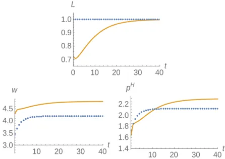
0 10 20 30 40t 0.90 0.92 0.94 0.96 0.98 1.00 L 0 10 20 30 40t 4.4 4.5 4.6 4.7 4.8 w 0 10 20 30 40t 2.05 2.10 2.15 2.20 2.25 2.30 2.35 pH
Figure 3: Transitional dynamics for an initially capital-poor economy assuming labor market integration at = 0 (solid lines) and assuming that labor markets remain closed (dotted lines). Parameter configuration: = ∗ = = ∗ = 5,
0 = 08 ˜,
0 = 08 ˜.
, compared to the pre-integration case. In the displayed numerical example, there is emigration despite the price for housing being initially lower than in the foreign economy. The property
0 ∗arises because the stock of structures is low, implying
that the marginal product of land in the production of housing services is low. Notably, despite emigration, there is accumulation of both physical capital, , and structures, , reflecting the standard neoclassical convergence force (Rappaport, 2005). Because emigration reduces the investment incentives compared to the pre-integration case, both types of capital accumulate more slowly than in the pre-integration case, as displayed in the Online Appendix. That is, the causal effect of emigration is to lower investment in both sectors. Over time, and after the initial drop of population density, the size of the workforce rises along with accumulation of physical capital and structures from = 1 onwards. This is the reverse migration phenomenon we observe in East Germany, according to Fig. 1 and 2, particularly in cities that are the economically most active regions. The price of housing services, , is lower on impact than it
would be in the closed economy because of emigration. It then rises over time because of increased demand for housing that is associated with increasing wages and (for the solid line) the reversal of the migration flows to immigration. The transition to the steady state level ˆ is slower than without labor market integration, where the labor
force is higher. 0 10 20 30 40t 0.7 0.8 0.9 1.0 L 10 20 30 40t 3.0 3.5 4.0 4.5 w 10 20 30 40t 1.4 1.6 1.8 2.0 2.2 pH
Figure 4: Transitional dynamics for an economy that initially is capital-poor and has low TFP levels assuming labor market integration at = 0 (solid lines) and as-suming that labor markets remain closed (dotted lines). Parameter configuration: 0 = 096∗ = 48, 0 = 096∗ = 48, 0 = 055 ˜, 0 = 085 ˜. and increase
according to a logistic function to 100 percent of the foreign TFP level only for the case of labor market integration (solid lines).
The experiment displayed in Fig. 4 not only assumes that initial state variables start below the pre-integration steady state values (0 = 055 ˜ and 0 = 085 ˜). It
also assumes that domestic TFP parameters start below the foreign levels (0 = 096∗
and 0 = 096∗). These border conditions capture the economic fundamentals of the
East German economy at the time of the reunification most accurately. For the long run, we assume that TFP levels converge gradually to 100 percent of the foreign level (lim→∞ = ∗ and lim→∞ = ∗). Increasing TFP levels over time are certainly
transfers and institutional improvements from advanced economies to East Germany (particularly from West German firms that opened plants in the New Laender after 1990). Physical capital and structures decumulate for a while shortly after labor market integration, whereas the stocks accumulate in the pre-integration case (as displayed in the Online Appendix) due to a standard neoclassical convergence mechanism. When TFP levels become sufficiently high, there is again a reversal of migration flows in parallel with rising wage rates, a rising price for housing services, and rising capital stocks.
Only if TFP levels remain sufficiently low also in the long run, it is possible that ˜
0 ˆ and ˜ 0 ˆ. In this case, emigration and decumulation of
capital occurs at the same time and there is no reverse migration. In the case of East Germany, however, there was technology transfer from advanced regions, foremost West Germany, along with capital accumulation. Hence, the premises underlying Fig. 4 are more plausible.
4.3
Reverse Migration: The Role of the Housing Sector
In a one-sector model, with the tradable goods sector only (i.e. = 1), the no-arbitrage condition V=V∗ that makes workers indifferent between migrating and staying in an
integrated labor market boils down to wage rate equalization, = ∗. As the wage
rate equals the marginal product of labor, it holds that ·()1− = ∗·(∗∗)1−.
Suppose again that labor markets integrate in period = 0. Also suppose that, one period in advance (in = −1), we have · (−1−1)1− ∗ · (∗∗)1−. Then,
in = 0, the capital stock remains at the previous level at all times and labor moves out with constant population thereafter. Formally, for all ≥ 0, we have = −1,
sustained by gross investment
=
−1, and = (∗)
1
1−−1∗∗ −1.
In other words, the economy − that may have been on a transition path with gradual capital accumulation before labor markets integrate − jumps into the steady state by adjusting the amount of workers through emigration at the time of labor markets integration. This is similar to the case in Burda (2006). A reversal of migration flows
over time cannot occur.
In the one-sector model of Rappaport (2005), there are exogenous limits to labor force adjustments each period such that emigration is stretched over time until wage rates have converged. A reversal of migration flows cannot occur either.
Reverse migration occurs in our model because of the presence of the housing sector. In the case where housing costs are lower in the domestic economy (as in Fig. 3 and 4), emigration early in the transition in response to labor market integration does not occur to a point where the domestic wage rate rises to the foreign level, despite the absence of exogenous migration costs.
5
Empirical Evidence: The Case of East Germany
In this section, we argue that the reverse migration scenario displayed in Fig. 3 and 4 is consistent with the evidence on net migration flows, the evolution of wages and the evolution of housing costs in the New German Laender after the fall of the Berlin Wall. Details on the data construction and robustness checks are relegated to the Online Appendix.
5.1
Net Migration Flows
Fig. 1 and 2 in the introduction are based on a new data set on net migration flows for the period 1991-2014 at the district level in East Germany. So far, the data were not publicly available for any district in the New Laender before 1995 and were also not available for most districts after 2007.19
The migration data set used for Fig. 1 and Fig. 2 is based on net migration balances, accounting for movements across the borders of administrative districts (NUTS 3 units in the EUROSTAT typology for all five New Laender in Germany). The districts in the New Laender were subject to numerous border reforms between 1991 and 2014,
19The reason for this limited data availability up to now were subsequent changes in county borders resulting from administrative reforms. We worked with the Statistical Offices of the New Laender to complete the data set. Their collaboration with us is gratefully acknowledged.
reducing their number considerably. To get consistent data over the entire period 1991 to 2014, one territorial status was chosen and reconstructed for the periods with differing district borders. The longest period not marked by significant territorial reforms lasted from 1995 to 2006. Thus, we selected the territorial boundaries during that period of time. For the periods before (1991-1994) and after the reference period (2007-2014), the municipalities (corresponding to LAU2 units) were assigned to the districts to whom they belonged during the reference period and their net migration balances were added up to reconstruct the data at the district-level.
To sum up the discussion in the introduction, we see a reversal of migration flows particularly in East German cities. Fig. 4 based on the theoretical model suggests that outflows are highest early in the transition, whereas Fig. 1 and 2 shows that migration outflows was higher in the second half than in the first of the 1990s. This may not only reflect a kind of behavioral inertia of workers, especially in more rural areas (Burda, 1993), but may also reflect massive public investment in the early 1990s in East Germany ("Aufbau Ost"), as discussed in OECD (2001). Overall, Fig. 3 and 4 are consistent with the evidence on the decline in emigration flows and an eventual reversal to net inflows.
5.2
Wages
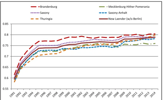
Fig. 3 and 4 also suggest that the reverse migration pattern is associated with gradual increases in both wage rates and rental rates of housing that are pronounced in the early transition phase. According to Fig. 5, the average wage income per worker in all the New Laender shows incomplete convergence to the West German level.
Wages increased particularly fast in the 1990s. Not all of that was market-driven, as trade unions pushed to harmonize wages in Germany. This was associated with comparatively high unemployment rates in East Germany. Consistent with the theo-retical considerations, however, wages in the Eastern Laender relative to the Western German wage level continued to increase (along with a decline in unemployment rates) in the 2000s as well, suggesting that TFP levels do not yet coincide.
0.55 0.6 0.65 0.7 0.75 0.8 0.85
Brandenburg Mecklenburg-Hither Pomerania Saxony Saxony-Anhalt
Thuringia New Laender (w/o Berlin)
Figure 5: Real wage income per worker relative to West Germany (without Berlin) in the New Laender, 1991-2014. Data: Federal Ministry of Finance, Germany.
5.3
Rental Rates for Housing
Finally, we relate the evolution of rental rates for housing over time in the New Laender to our model, by constructing a comprehensive data set on rental housing in East Germany that has not yet been used elsewhere (for West Germany, see Fitzenberger and Fuchs, 2016). The data on housing costs come from the German Socio-Economic Panel Study (SOEP), a representative annual household panel survey that offers detailed information on rental housing from the perspective of tenants. The final data set consists of 107,514 private households who live in rental apartments between 1984 and 2014 in West Germany and 34,248 private households who live in rental apartments between 1990 and 2014 in East Germany.
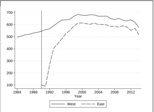
Fig. 6 visualizes the evolution of the "raw" average monthly rental payments per square metre for East Germany (since 1990) and West Germany (since 1984) over time, employing the full sample. While West German rental rates show no trend since the early 1990s (consistent with a steady state), the price for housing services increased fast in East Germany in the 1990s. In the 2000s it was six times as high as in 1990.
100 200 300 400 500 600 700 1984 1988 1992 1996 2000 2004 2008 2012 Year West East
Figure 6: Evolution of raw average rental payments per square meter per month in East Germany vs. West Germany. Note: Index with the average rent in East Germany in year 1990 as basis value (= 100). Data: German Socio-Economic Panel (SOEP), version 31.
As for wages, we observe incomplete convergence to West German levels.20
Fig. 7 shows the evolution of average rental payments per square metre for the New Laender (including East Berlin) based on a standard hedonic pricing model that accounts for variation in apartment quality. We control for the year of construction, the type of location area (new residential, old residential, mixed or other), the general apartment condition, and whether the apartment is equipped with a garden, a bal-cony/terrace, central heating and a basement. Because of the panel structure of the data, we are also able to control for fixed effects at the apartment level.21 Comparing Fig. 7 to Fig. 6 shows that the evolution of quality-adjusted housing costs is similar
20The speed of the increase in the 1990s was certainly slowed down by regulations that limited upward rent adjustments, especially but not exclusively for those already living in the same apartment before October 1990 (Neumann and Schaper, 2008). These special regulations ended in January 1998 after which the regulations coincided with those in West Germany (i.e. rental rates for housing must not exceed a certain percentage of the local average for comparable apartments).
21The Online Appendix describes the underlying estimation procedure and the data in detail. We also present further results that demonstrate robustness.
100 200 300 400 500 1984 1988 1992 1996 2000 2004 2008 2012 Year
Berlin−East Brandenburg Mecklenburg−HP Saxony Saxony−Anhalt Thuringia
Figure 7: Evolution of quality-adjusted average rental payments per square meter in the New Laender. Note: Index with the average rent in East Germany in year 1990 as basis value (= 100). Data: German Socio-Economic Panel (SOEP), version 31.
to the raw average in East Germany in Fig. 6 across all New Laender (including East Berlin).
The evolution of in Fig. 3 and 4, based on the reverse migration case of the
theoretical model, is qualitatively consistent with Fig. 6 and 7, particularly for the 1990s where we see gradual increases in rental rates for East Germany. The reason why rental rates have been rather flat during the 2000s (while the theoretical model would predict further increases) may be rooted in new rental price regulation policy, beside slow economic growth in Germany as a whole during the 2000s. In a study for the Old Laender, Fitzenberger and Fuchs (2016) show that the tenancy law reform act in 2001 reduced apartment rents significantly for new leases. The negative reform effect diminishes with the duration of a tenancy. Thus, households who live in tenancies that are affected by the reform benefit less from being sitting tenants than households in tenancies that started before September 2001. However, there are also regulations that limit rental rate increases for sitting tenants in Germany. These regulations may have
contributed to slow growth of rental rates after 2001 for reasons that are not captured in our simple theoretical model.
6
Conclusion
This paper has examined the impact of labor market integration on migration, capital formation, wages, the rental rate of land, and the price for housing services in an intertemporal model with a tradable goods sector and a housing sector. Our framework is capable to explain the phenomenon of reverse migration patterns that, for instance, occurred in (urban) East Germany in the aftermath of the sudden fall of the iron curtain (and the Berlin wall) in 1989. The reverse migration scenario is driven by low initial capital stocks and possibly also by low productivity levels that are increasing over time. The mechanism which acts as a drag on migration flows and prevents that everyone moves to high-income regions, once this is legally made feasible, works through the relative price of housing across regions. Once labor productivity is rising over time, the migration flow may reverse despite the co-evolution of rising housing costs. According to the best of our knowledge, previous studies based on neoclassical models were unable to explain that labor market integration may lead to labor outflows in early phases and immigration in later phases of the transition to the new long run equilibrium. The reverse migration scenario has suggested an evolution of wages and rental rates of housing that is consistent with the evidence for post-unification East Germany, exploiting the unique case of complete labor market integration and institutional harmonization across regions.
More generally, we have examined how initial conditions (i.e. initial levels of popu-lation density, productivity levels, and capital stocks) affect the direction of migration flows over time along with other key variables. We have demonstrated that capital inflows and emigration can occur at the same time, leading to a reversal of migration flows in the aftermath. Our analysis also suggests that, nevertheless, the causal effect of immigration on capital investments, the land price and housing costs is unambiguously
the price for housing services, and residential capital investment by helping to address potential endogeneity biases.22
Future research may exploit our setup to study the political economy side of mi-gration policy.23 Heterogeneity in the ownership of land may be important for distrib-utional consequences in response to labor market integration, caused by changes in the rental rate of land and housing costs. This may help to understand political debates on and resistance to immigration even when migration inflows have negligible effects on the domestic labor market.24
Appendix
Derivation of (16). We omit household index and solve the household’s problem in two steps. In the first step, the intertemporal consumption problem is solved. Define a Cobb-Douglas consumption index, C := 1− such that instantaneous utility is given
by log C. Consumption expenditure in a given period can be expressed as
· C = + (20)
where denotes an appropriately defined price index (see below). Life-time utility of an individual born in reads as = logC1+ logC2+1.
For later use, we also allow for second-period income. Denote income of an
indi-22Empirical studies have emphasized the role of wage differences across regions (e.g. Grogger and Hanson, 2011) and the role of migrant networks (Beine, Docquier and Ozden, 2011) for migration flows. We emphasize the need to account for differences in housing costs as well.
23See e.g. Benhabib (1906) for an important study based on heterogeneity of capital holdings of both natives and immigrants. De la Croix and Docquier (2014) propose a very interesting recent political economy perspective of a host country. In their model, higher immigration in a single country does not raise welfare from a nationalist point of view whereas a coordinated increase in immigration quotas of a group of rich countries may lead to a Pareto improvement under an appropriate tax-subsidy scheme. In our set up, the challenge would be to achieve a Pareto improvement within a region when immigration produces winners and losers.
24Switzerland would be a prime example. In a widely discussed referendum on February 9, 2014, Switzerland voted for restricting immigration by opting out of its bilateral agreement with the Euro-pean Union on the free movement of labor (with a 50.3 percent majority). This was seen as remarkable by commentators, as labor market effects were largely invisible despite massive immigration since the agreement came into full effect in 2007. However, the main discussion in Switzerland centered on rising prices for housing services.
vidual born in in the first and second period of life by 1 and 2+1, respectively.
Moreover, define
≡ 1+
2+1
1 + (21)
First-period income is equal to the wage rate, 1 = . Let denote individual
savings in working age at time , i.e. := − 1C1. We have
C1 = − 1 (22) C2+1= (1 + ) + 2+1 2+1 (23)
The intertemporal problem may be expressed as follows:
max
{log (
− )− log (1) + log [(1 + ) + 2+1]− log (2+1)} (24)
The first-order condition with respect to savings implies
1C1 = 1 1 + (25) 2+1C2+1 1 + = 1 + (26)
In the second step, we analyze the static problems. Given the amount of first-period consumption expenditure in (25), the household solves
max 11 log£(1)(1)1− ¤ s.t. 1 1 + = 1+ 1 (27) Hence, 1= 1− 1 (28)
which combined with the first-period budget constraint in (27) implies
1 = 1 + 1= 1− 1 + (29)
Similarly, given the amount of second-period consumption expenditures in (26), the household solves max 2+12+1 log£(2+1)(2+1)1− ¤ s.t. (1 + ) 1 + = 2+1+ +12+1 (30) Hence, we get 2+1 = 1− +12+1 (31)
which combined with (1 + ) = 1 and the second-period budget constraint in (30) leads to 2+1= 1 + 2+1= 1− 1 + +1 (32)
Inserting (29) and (32) into the intertemporal utility function (12) confirms (16). It remains to be shown that there exists a price index as used above. Using = 1−, the price index may be expressed as
= + C = ³ ´1− + µ ¶ (33)
Noting that = 1− one gets
=¡¢1− "µ 1− ¶1− + µ 1− ¶# (34)
This concludes the proof. ¥
Proof of Proposition 1. Denote by the shadow price of physical capital
in numeraire sector, i.e. the multiplier to capital accumulation constraint (3) in the profit maximization problem (2) of firms in the numeraire goods sector. The associated Lagrangian function is given by
L ≡ ∞ X =0 µ 1 1 + ¶¡ ·¡ ¢ ()1−− − ∙ 1 + µ ¶¸ + ·£+¡1− ¢− +1 ¤¶ (35)
The associated first-order conditions L = L = L +1 = 0 imply · · µ ¶1− = (36) = µ − 1 ( + 1) ¶1 (37) (1− )+1 + (1− ) · · µ +1 +1 ¶ + µ +1 +1 ¶+1 = (1 + ) (38)
According to (9), we have the following first-order conditions of the representative housing services firm:
µ ¶−1 = (39) = µ (1− ) ¶1 (40)
Combining (39) and (40) yields
= ( )1 µ 1− ¶1− (41)
Denote by the shadow price of structures, i.e. the multiplier to constraint (6) in
the profit maximization problem (7) of construction firms. The associated Lagrangian function is given by L ≡ ∞ X =0 µ 1 1 + ¶¡ − − + · h ¡ ¢ ()1− + ¡ 1− ¢− +1 i´ (42)
The associated first-order conditions L = L = L +1 = 0 imply · · · µ ¶−1 = (43)
= 1 · (1 − ) µ ¶ (44) +1+ (1− )+1 = (1 + ) (45)
Combining (43) with (44) and using (36) implies
· · µ ¶1− = 1− (46)
Combining (44) with (45) and using (41) implies
· (1 − ) (+1) 1 µ 1− +1 ¶1− + (1− ) µ +1 +1 ¶ = (1 + ) µ ¶ (47)
Combining and (37) with (38) leads to
(1− )+1 + (1− ) · · µ +1 +1 ¶ + 1 µ +1− 1 + 1 ¶+1 = (1 + ) (48)
Combining (3) and (37) we can write +1 = µ − 1 ( + 1) ¶1 + 1− (49)
The market clearing condition for non-tradables reads as
= Z 0 1()di + Z −1 0 2()di (50)
According to (29), (32) and (11), demand for the non-tradable good of a young and an old individual in period , with landholding () in the second period of life, is
1() = 1− 1 + + +1() 2() = 1− 1 + −1+ () (51)
respectively, where we used (14). Substituting (51) into (50) and using (8) yields µ ¶ = 1− 1 + + −1 −1 + ( +1+ ) (52) Using (40) in (52) leads to = (1− ) (1 − ) 1 + ∙ + −1 −1 + · ( +1+ ) ¸ (53)
Recall notation = , = , = , = and = . Also
let ≡ . Prior to labor market integration, for a given sequence of cohort sizes per unit of land, {}∞=−1, the sequences of quantities { +1 +1}∞=0 and prices
{ }∞=0 are given by +1= ¡ ¢()1− + (1− ). (54) + = (55) +1 = µ − 1 ( + 1) ¶1 + 1− (56) = · · µ ¶1− (57) = µ (1− ) ¶1 (58) · (1 − ) (+1)1 µ 1− +1 ¶1− + (1− ) µ +1 +1 ¶ = (1 + ) µ ¶ (59) (1− )+1 + (1− ) · · µ +1 +1 ¶ + 1 µ +1− 1 + 1 ¶+1 = (1 + ) (60) = (1− ) (1 − ) 1 + £ + −1−1+ (+1+ ) ¤ (61) · · µ ¶1− = 1− (62)
then give us the sequence {
}∞=0 according to (41) and, using (44), the sequence
{ }∞=0 according to = 1 · (1 − ) µ ¶ (63)
In long-run equilibrium, the values of quantities {
} and prices {
} are time-invariant. According to (56), we obtain the long run shadow values of physical capital as
˜ = 1 + ( + 1)¡¢ (64) Using (64) in (60) gives us ˜ ˜ = Ã (1− ) · + + ( + 1)¡¢+ ¡¢+1 !1 (65) Let us define Ω≡ Ã 1− + + ( + 1)¡¢ + ¡¢+1 !1− (66)
Substituting (65) into (57) leads to
˜
= Ω· 1 (67)
Substituting (65) into (46) we obtain ˜ ˜ = 1− Ω· 1 (68) Using (68) in (63), we find ˜ = −(1− )−(1−)Ω · (69)
popula-tion density reads as = 2. Substituting (67) into (61), we obtain the long run rental rate of land as ˜ = (1− ) (1 − ) 1 + − 2 (1 − ) (1 − )Ω· 1 · (70)
Using (68) and (70) into (59), in long run equilibrium,
˜ = Ã + (1− )1− · !µ (1− ) · 1 + − 2 (1 − ) (1 − ) ¶1− Ω1−(1−)· 1−(1−) (71) Using (70) and (71) in (41), we obtain
˜
=¡ + ¢−(1− )−(1−)Ω ·
(72)
Using (70) and (71) in (58), we obtain
˜ = (1 − )1− (1− ) 1 + − 2 (1 − ) (1 − ) Ω1− + · 1− · · (73)
Moreover, according to (54) and (68), ˜ = ˜ ³1− Ω· 1 ´1− = (1− ) 1 + − 2 (1 − ) (1 − ) + · (74)
where the latter follows after substituting (73).25 Substituting (74) into (55), we find
˜ = − ˜ = µ 1− 2 (1− ) 1 + − 2 (1 − ) (1 − ) + ¶ · 2 (75) With these expressions, it is easy to confirm comparative-static results. ¥
Proof of Proposition 2. With integrated labor markets, recalling ∆ = 0,
equi-25For an interior long run equilibrium to exist, it must hold that ˜(2) , i.e. (1 − ) 1 + − 2 (1 − ) (1 − ) + 1 2
librium condition (17) that governs migration holds, i.e., log³ ∗ ´ = (1− ) · log³ ∗ ´ + log³+1 ∗ ´ 1 + (76)
according to (16), where ∗ and ∗ are the wage rate and price for housing services in
the foreign economy. Since the foreign economy is in steady state by assumption and differs from the domestic economy in productivity parameters (∗ ∗)and population
density ∗ only. Thus, according to (67) and (71), we have
˜ ∗ = µ ∗ ¶1 (77) ˜ ∗ = µ ∗ ¶1−(1−) (78)
respectively. Let us denote the long run population density with integrated labor markets by ˆ. Using (77) and (78) in (76), we obtain
ˆ ∗ = ¡ ∗ ¢+(1−)(1−) (1−)(1−) ¡∗ ¢ 1− (79)
This confirms comparative-static results. ¥
References
[1] Abel, Andrew B. (1982). Dynamic Effects of Permanent and Temporary Tax Poli-cies in a q Model of Investment, Journal of Monetary Economics 9, 353—373. [2] Armenter, Roc and Francesc Ortega (2011). Credible Redistribution Policies and
Skilled Migration. European Economic Review 55, 228-245.
[3] Beine, Michel, Frédéric Docquier and Caglar Ozden (2011). Diasporas, Journal of Development Economics 95, 30-41.