Recovering portfolio default intensities implied by CDO quotes

HAL Id: hal-00413730

https://hal.archives-ouvertes.fr/hal-00413730

Submitted on 6 Sep 2009

HAL is a multi-disciplinary open access

archive for the deposit and dissemination of

sci-entific research documents, whether they are

pub-lished or not. The documents may come from

teaching and research institutions in France or

L’archive ouverte pluridisciplinaire HAL, est

destinée au dépôt et à la diffusion de documents

scientifiques de niveau recherche, publiés ou non,

émanant des établissements d’enseignement et de

recherche français ou étrangers, des laboratoires

Recovering portfolio default intensities implied by CDO

quotes

Rama Cont, Andreea Minca

To cite this version:

Rama Cont, Andreea Minca. Recovering portfolio default intensities implied by CDO quotes.

Math-ematical Finance, Wiley, 2013, 23 (1), pp.94-121. �10.1111/j.1467-9965.2011.00491.x�. �hal-00413730�

Recovering portfolio default intensities

implied by CDO quotes

∗

Rama CONT

Andreea MINCA

Revised version. First version appeared as: Columbia Financial

Engineering Report No. 2008-01, Jan 2008.

Abstract

We propose a stable non-parametric algorithm for the calibration of pricing models for portfolio credit derivatives: given a set of observations of market spreads for CDO tranches, we construct a risk-neutral default intensity process for the portfolio underlying the CDO which matches these observations, by looking for the risk neutral loss process ’closest’ to a prior loss process, verifying the calibration constraints. We formalize the problem in terms of minimization of relative entropy with respect to the prior under calibration constraints and use convex duality methods to solve the problem: the dual problem is shown to be an intensity control problem, characterized in terms of a Hamilton–Jacobi system of differen-tial equations, for which we present an analytical solution. Given a set of observed CDO tranche spreads, our method allows to construct a default intensity process which leads to tranche spreads consistent with the ob-servations. We illustrate our method on ITRAXX index data: our results reveal strong evidence for the dependence of loss transitions rates on the past number of defaults, thus offering quantitative evidence for contagion effects in the risk–neutral loss process.

Keywords: collateralized debt obligation, duality, portfolio credit derivatives, reduced-form models, default risk, intensity control, top-down credit risk mod-els, relative entropy, inverse problem, model calibration, stochastic control.

∗_{This work was presented at the at the Workshop on PDEs in finance (Stockholm Aug}

2007), the Stanford Financial mathematics seminar (Oct 07), Conference on Credit Risk (Chicago Univ, Oct 07), the CCCP 2007 Conference (Princeton Nov 07), the S&P Credit Risk Summit (New York Nov 07) the Conference on Credit Risk (Evry 2008) Bachelier Congress 2008 and the Chicago University Credit Risk conference (2008). We thank Marco Avellaneda, Damiano Brigo, Bruno Dupire, YuHang Kan, Johannes Ruf, Kay Giesecke and Igor Halperin for helpful remarks.

Contents

1 Introduction 3

2 Portfolio credit derivatives 4

2.1 Index default swaps . . . 5

2.2 Collateralized Debt Obligations (CDOs) . . . 5

2.3 Top-down models for CDO pricing . . . 6

3 The information content of CDO tranches 9 3.1 Mimicking marked point processes with Markovian jump processes 9 3.2 Information content of portfolio credit derivatives . . . 11

4 The calibration problem 12 4.1 Calibration as relative entropy minimization under constraints . 12 4.2 Computation of the relative entropy . . . 13

4.3 Dual problem as an intensity control problem . . . 15

4.4 Hamilton Jacobi equations . . . 16

4.5 Handling payment dates . . . 18

5 Recovering market-implied default rates 19 5.1 Calibration algorithm . . . 19

5.2 Application to ITRAXX tranches . . . 20

1

Introduction

Credit derivatives markets have witnessed an extraordinary activity in the last decade, especially with the development of a large market in portfolio credit derivatives of which collateralized debt obligations (CDOs) are the most well known example [8]. Yet, as illustrated in the recent market turmoil, commonly used modeling approaches –mostly static, copula-based pricing models such as the Gaussian copula model– appear to be insufficient for pricing and hedging these complex derivatives. One of the reasons has been the lack of transparency of such pricing methods in which non-intuitive and unobservable “default cor-relation” parameters are required as an input.

The Gaussian copula model, which has been widely used for the pricing of CDOs, has some well known shortcomings: its inability to reproduce market val-ues of CDO tranche spreads, as exemplified by the base correlation skew, the in-stability of its “default correlation” parameters –as revealed by the GM/FORD crisis in May 2005 and the subprime crisis in 2007– and, most importantly, the lack of a well-defined dynamics for the risk factors which prevents any model-based assessment of hedging strategies. Other copula-model-based models may provide better fits to market quotes but share the other drawbacks of the Gaussian cop-ula model, most notably its static character. These shortcomings have inspired a lot of research on alternative approaches to credit risk modeling [24]. On the other hand, a great advantage of static copula models is the ease with which the parameters can be calibrated to market data: this is a feature which many of the more complex, multi-name dynamic models such as Duffie & Garleanu [16], have lacked so far. The key challenge in improving on the Gaussian copula model lies therefore not so much in adding more realistic features to the model but in adding these features while maintaining analytical tractability, especially in regard to the calibration to market data.

To tackle some of these issues while allowing for a parsimonious parametriza-tion of the model, several recent works [28, 21, 19, 1, 25] have proposed a “top-down” approach to the problem, in which one models in “reduced form” the dynamics of the portfolio loss, as a jump process whose intensity 𝜆𝑡 represents

the (conditional) rate of occurrence of the next default and whose jump sizes represent the losses given default. Though top-down pricing models are typ-ically much simpler to simulate or implement than high-dimensional reduced form models, numerical methods –Laplace transforms, numerical resolution of ODEs– are still required for the pricing of CDO tranches which makes parameter calibration computationally challenging. Existing studies of top-down pricing models [28, 21, 19, 1, 25] address model calibration by applying black box op-timization procedures, whose convergence is not guaranteed, to the resulting high-dimensional nonlinear optimization problems. The lack of convexity of the optimization problems involved may lead to multiple solutions and numerical sensitivity of the results, making such results difficult to reproduce and render-ing their interpretation delicate.

In this work we propose a rigorous nonparametric approach to the calibration of “top-down” pricing models for portfolio credit derivatives to a set of observed

CDO tranche spreads. First, we show a “mimicking theorem” for point processes which states that the marginal distributions of a loss process with arbitrary stochastic intensity can be matched using a Markovian point process. This result implies that, given any risk-neutral loss process with given default intensity we can construct a Markovian loss process which leads to the same prices. This observation allows to narrow down the calibration problem to the search for a Markovian loss process verifying a set of calibration constraints. We formalize this problem in terms of the minimization of relative entropy with respect to the law of a prior loss process under calibration constraints. We use convex duality techniques to solve the problem: the dual problem is shown to be an intensity control problem, characterized in terms of a Hamilton-Jacobi system of differential equations which can be analytically solved using a change of variable. Given a set of observed CDO tranche spreads, our method allows to construct an implied intensity process 𝜆𝑡 which leads to tranche spreads consistent with

the observations. The implied intensity 𝜆𝑡= 𝑓 (𝑡, 𝐿𝑡) depends on the defaults

in the portfolio, which naturally leads to ’contagion’ effects in the occurrence of defaults. The resulting model is parameterized by the probability (per unit time) of the next default in the portfolio, which allows for an intuitive check on parameter values.

The article is structured as follows. Section 2 describes the cash flow struc-ture of a (static) CDO and present a brief review of the “top-down” modeling approach for portfolio credit derivatives. In section 3 we discuss the level of in-formation about the risk-neutral loss process which can be extracted from CDO tranches: we state a “mimicking theorem” for point processes which implies that, in a general setting, the information content of CDO tranche quotations can be represented in the form of an effective intensity function allowing for de-pendence of the default rate on the current number of defaults in the portfolio and calendar time. The model calibration problem is defined in section 4 and formulated in terms of relative entropy minimization under constraints. In sec-tion 4.3 we show that, via convex duality, the calibrasec-tion problem maps into an intensity control problem for a point process, which is then solved using dynamic programming. These results translate into a calibration algorithm which can be used to extract the risk–neutral default intensity from CDO tranche spreads: the algorithm is laid out in detail in section 5 and applied to ITRAXX index data. Section 6 discusses the implications of our results.

2

Portfolio credit derivatives

Let (Ω, (ℱ𝑡)𝑡≤𝑇) be the set of market scenarios endowed with a filtration (ℱ𝑡)0≤𝑡≤𝑇

representing the flow of information with time. Consider a reference portfolio on which the credit derivatives we consider will be indexed. The main object of interest are the number of defaults 𝑁𝑡and the (cumulative) default loss 𝐿𝑡

of this reference portfolio during a period [0, 𝑡]. Although the discussion below can be generalized to account for correlation between interest rates and default rates, for simplicity we shall assume independence between default risk and

in-terest rate risk. We denote by 𝐵(𝑡, 𝑇 ) the discount factor at date 𝑡 for the maturity 𝑇 ≥ 𝑡.

A portfolio credit derivative can be modeled as a contingent claim whose payoff is a (possibly path-dependent) function of the portfolio loss process

(𝐿𝑡)𝑡∈[0,𝑇 ]. The most important example of portfolio credit derivatives are index

default swaps and collateralized debt obligations (CDO) [8].

2.1

Index default swaps

Index default swaps are now commonly traded on various credit indices such as ITRAXX and CDX series, which are equally weighted indices of credit default swaps on European and US names [8]. In an index default swap transaction, a protection seller agrees to pay all default losses in the index (default leg) in return for a fixed periodic spread 𝑆 paid on the total notional of obligors remaining in the index (premium leg). Denoting by 𝑡𝑗, 𝑗 = 1..𝐽 the payments

dates,

∙ the default leg pays at 𝑡𝑗 the losses 𝐿(𝑡𝑗) − 𝐿(𝑡𝑗−1) due to defaults in

]𝑡𝑗−1, 𝑡𝑗]

∙ the premium leg pays at 𝑡𝑗 an interest (spread) 𝑆 on the notional of the

remaining obligors

(𝑡𝑗− 𝑡𝑗−1)𝑆(1 −

𝑁𝑡𝑗

𝑛 ). (1)

In particular the cash flows of the index default swap only depend on the port-folio characteristics via 𝑁𝑡 and 𝐿𝑡. The value at 𝑡 = 0 of the default leg is

therefore 𝐽 ∑ 𝑗=1 𝐸ℚ_{[𝐵(0, 𝑡} 𝑗)(𝐿(𝑡𝑗) − 𝐿(𝑡𝑗−1)]

while the value at 𝑡 = 0 of the premium leg is 𝑆 𝐽 ∑ 𝑗=1 𝐸ℚ_{[𝐵(0, 𝑡} 𝑗)(𝑡𝑗− 𝑡𝑗−1)(1 − 𝑁𝑡𝑗 𝑛 )].

The index default swap spread at 𝑡 = 0 is defined as the (fair) value of the spread which equalizes the two legs at inception:

𝑆index= 𝐸ℚ_[∑𝐽 𝑗=1𝐵(0, 𝑡𝑗)(𝐿(𝑡𝑗) − 𝐿(𝑡𝑗−1) )] ∑𝐽 𝑗=1𝐸ℚ[𝐵(0, 𝑡𝑗)(𝑡𝑗− 𝑡𝑗−1)(1 − 𝑁_𝑡𝑗 𝑛 )] . (2)

2.2

Collateralized Debt Obligations (CDOs)

Consider a tranche defined by an interval [𝑎, 𝑏], 0 ≤ 𝑎 < 𝑏 < 1 for the loss process normalized by the total nominal. A CDO tranche swap (or simply CDO tranche)

is a bilateral contract in which an investor sells protection on all portfolio losses within the interval [𝑎, 𝑏] over some time period [0, 𝑡𝐽] in return for a periodic

spread 𝑆(𝑎, 𝑏) paid on the nominal remaining in the tranche after losses have been accounted for.

The loss of an investor exposed to the tranche [𝑎, 𝑏] is

𝐿𝑎,𝑏(𝑡) = (𝐿𝑡− 𝑎)+− (𝐿𝑡− 𝑏)+. (3)

The premium leg is represented by the cash flow payed by the protection buyer to the protection seller. In case of a premium S, its value at time 𝑡 = 0 is

𝑃 (𝑎, 𝑏, 𝑡𝐽) = 𝐽

∑

𝑗=1

𝑆(𝑡𝑗− 𝑡𝑗−1)𝐸ℚ[𝐵(0, 𝑡𝑗)((𝑏 − 𝐿(𝑡𝑗))+− (𝑎 − 𝐿(𝑡𝑗))+ )]

The default leg is represented by the cash payed by the protection seller to the protection buyer in case of default. Its value at time 𝑡 = 0 is

𝐷(𝑎, 𝑏, 𝑡𝐽) = 𝐽

∑

𝑗=1

𝐸ℚ[𝐵(0, 𝑡𝑗)(𝐿𝑎,𝑏(𝑡𝑗) − 𝐿𝑎,𝑏(𝑡𝑗−1) )].

The “fair spread” (or simply, the tranche spread) is the premium value 𝑆0(𝑎, 𝑏, 𝑡𝐽)

that equates the values of the two legs: 𝑆0(𝑎, 𝑏, 𝑡𝐽) = 𝐸ℚ ∑𝐽 𝑗=1𝐵(0, 𝑡𝑗)[𝐿𝑎,𝑏(𝑡𝑗) − 𝐿𝑎,𝑏(𝑡𝑗−1) ] 𝐸ℚ ∑𝐽 𝑗=1𝐵(0, 𝑡𝑗)(𝑡𝑗− 𝑡𝑗−1)[(𝑏 − 𝐿(𝑡𝑗))+− (𝑎 − 𝐿(𝑡𝑗))+] . Table 1 gives an example of such a tranche structure and the corresponding spreads for a standardized portfolio, the ITRAXX index. Note that these ex-pressions for the tranche spreads depend on the portfolio loss process via the expected tranche notionals 𝐶(𝑡𝑗, 𝐾) where

𝐶(𝑡, 𝐾) = 𝐸ℚ[(𝐾 − 𝐿𝑡)+]. (4)

2.3

Top-down models for CDO pricing

It is immediately observed that the above expressions for the spread of a CDO tranche depend on the portfolio characteristics only through the (risk-neutral) law of the loss process 𝐿𝑡. The idea of “top-down” pricing models [1, 19, 21, 25,

28] is to model the risk neutral loss process, either by specifying the dynamics of the cumulative loss [1, 19, 21, 25] or by looking at the forward loss distribution [28]. We adopt here the former approach, which is simpler to implement.

The loss 𝐿𝑡is a piecewise constant process with upward jumps at each default

event: its path is therefore completely characterized by the default times (𝜏𝑗)𝑗≥1,

representing default events and the jump sizes Δ𝐿𝑗 representing the loss given

Maturity Low High Bid∖ Upfront Mid∖ Upfront Ask∖ Upfront 5Y 0% 3% 11.75% 11.88% 12.00% 3% 6% 53.75 54.50 55.25 6% 9% 14.00 14.75 15.50 9% 12% 5.75 6.25 6.75 12% 22% 2.13 2.50 2.88 22% 100% 0.80 1.05 1.30 7Y 0% 3% 26.88% 27.00% 27.13% 3% 6% 130 131.50 132 6% 9% 36.75 37.00 38.25 9% 12% 16.50 17.25 18.00 12% 22% 5.50 6.00 6.50 22% 100% 2.40 2.65 2.90 10Y 0% 3% 41.88% 42% 42.13% 3% 6% 348 350.50 353 6% 9% 93 94.00 95 9% 12% 40 41.00 42 12% 22% 13.25 13.75 14.25 22% 100% 4.35 4.60 4.85

Table 1: CDO tranche spreads, in bp, for the ITRAXX index on March 15 2007. For the equity tranche the periodic spread is 500bp and figures represent upfront payments.

index 𝑗 is not associated with the default of a given obligor but with the ordering in time of the events. The idea of aggregate loss models is to represent the rate of occurrence of defaults in the portfolio via the portfolio default intensity 𝜆𝑡:

we model the number of defaults (𝑁𝑡)𝑡∈[0,𝑇∗_] is a point process with ℱ𝑡-intensity

(𝜆𝑡)𝑡∈[0,𝑇∗_] under ℚ i.e.

𝑁𝑡−

∫ 𝑡

0

𝜆𝑡𝑑𝑡

is an ℱ𝑡-local martingale under ℚ [6]. Intuitively, 𝜆𝑡 can be seen as probability

per unit time of the next default conditional on current market information: 𝜆𝑡= lim

Δ𝑡→0

1

Δ𝑡 ℚ[𝑁𝑡+Δ𝑡= 𝑁𝑡+ 1∣ℱ𝑡]

Here ℱ𝑡represents the coarse-grained information resulting from the observation

of the aggregate loss process 𝐿𝑡 of the portfolio and risk factors affecting it. In

the simplest case it corresponds to the information (filtration) generated by the variables 𝜏𝑗, Δ𝐿𝑗but it may also contain information on other market variables.

This risk neutral intensity 𝜆𝑡can be interpreted as the short term credit spread

for protection against the first default in the portfolio [28].

𝜆𝑡 can be modeled as a stochastic process that may depend on the loss

process itself. The simplest specification is to model the loss 𝐿𝑡as a compound

Poisson process [7], but since the intensity is constant and independent of the loss process, this does not enable to model features such as spread volatility or default contagion [14]. Spread volatility can be introduced by modeling 𝜆𝑡as an

autonomous jump-diffusion process and then constructing 𝑁𝑡as a Cox process:

conditional on (𝜆𝑡)𝑡∈[0,𝑇∗], 𝑁 has the law of a Poisson process with intensity

(𝜆𝑡)𝑡∈[0,𝑇∗]. This approach, common in the credit risk literature, has been used

by Longstaff & Rajan [25] to model aggregate default rates in the CDX index. Default contagion can be incorporated in the model by introducing a dependence of the default intensity on the number of defaults. Ding et al. [15] construct the default process by starting from a linear birth process with immigration 𝜆𝑡 = 𝑐 + 𝑔𝑁𝑡 and applying a time change, while Arnsdorff & Halperin [1] use

a two factor specification: 𝜆𝑡 = 𝜆0(𝑁0− 𝑁𝑡)𝑌𝑡 where 𝑌𝑡 is a non-negative

stochastic process (see also [26]). Finally, one can argue that not only the occurrence of defaults but also their timing and magnitude can affect the default intensity: this feature has been modeled using Hawkes or self-exciting processes [19, 21].

Given the wide variety of models available for the default intensity, the choice of the model class among the above is not easy in practice. Indeed, even at the qualitative level it is not obvious which parametric specifications adequately reproduce observed features of market data. Also, once the class of models has been chosen, it is a nontrivial task to calibrate the model parameters in order to reproduce market spreads of index CDO tranches. In fact, in the models de-scribed above, numerical methods must be used to compute tranche spreads so the corresponding inverse problem of recovering parameters from market quotes is a computationally intensive one. Finally, these parameterizations mainly stem

from analytical convenience, more than from any fundamental economic consid-erations, so a nonparametric approach which makes fewer arbitrary assumptions on the form of the default intensity can provide some insight for model selection.

3

The information content of CDO tranches

One issue in the design and calibration of top-down models is how to parame-terize the portfolio loss process in a general, yet parsimonious, way which can be flexible enough to accommodate market observations of tranche spreads and remain tractable. The main issue is how to specify the dependence of the default intensity 𝜆𝑡with respect to other variables in the model: existing models range

from a deterministic intensity 𝜆(𝑡) to full path-dependence with respect to the loss process [19, 21].

While richer models might generate more realistic statistical features, an important issue in model calibration is the identifiability of such complex models. Given current prices of portfolio credit derivatives, what can be inferred from them in terms of the characteristics of the loss process? In this section we present a result which sheds light on this identifiability issue, showing that the marginal distributions of any marked point process with IID marks can be matched by a Markovian jump process. From this “mimicking theorem” we conclude that the retrievable information in the intensity process is exactly given by its conditional expectation given the loss process, which we call the effective intensity.

3.1

Mimicking marked point processes with Markovian

jump processes

We first show a “mimicking theorem” which shows that the marginal distri-butions of any marked point process with IID marks can be matched by a Markovian jump process:

Proposition 1. Consider any non-explosive jump process (𝐿𝑡)𝑡∈[0,𝑇∗] with a

intensity process (𝜆𝑡(𝜔))𝑡∈[0,𝑇∗_] and IID jumps with distribution 𝐹 . Define

( ˜𝐿𝑡)𝑡∈[0,𝑇∗_] as the Markovian jump process with jump size distribution 𝐹 and

intensity

𝜆eff(𝑡, 𝑙) = 𝐸ℚ[𝜆𝑡∣𝐿𝑡−= 𝑙, ℱ0] (5)

Then, for any 𝑡 ∈ [0, 𝑇∗_{], 𝐿}

𝑡 and ˜𝐿𝑡have the same distribution conditional on

ℱ0. In particular, the flow of marginal distributions of (𝐿𝑡)𝑡∈[0,𝑇∗] only depends

on the intensity (𝜆𝑡)𝑡∈[0,𝑇∗] through its conditional expectation 𝜆eff(., .).

We call (5) the effective intensity associated to the process 𝐿. The relation between the intensity 𝜆𝑡 and the effective intensity 𝜆eff(𝑡, 𝐿𝑡−) is analogous to

the relation between instantaneous volatility and local volatility in diffusion models [11, 17].

Proof. Consider any bounded measurable function 𝑓 (.). Using the pathwise decomposition of 𝐿𝑇 into the sum of its jumps we can write

𝑓 (𝐿𝑇) = 𝑓 (𝐿0) + ∑ 0<𝑠≤𝑇 (𝑓 (𝐿𝑠−+ Δ𝐿𝑠) − 𝑓 (𝐿𝑠−) ) (6) so 𝐸[𝑓 (𝐿𝑇)∣ℱ0] = 𝑓 (𝐿0) + 𝐸[ ∑ 0<𝑠≤𝑇 (𝑓 (𝐿𝑠−+ Δ𝐿𝑠) − 𝑓 (𝐿𝑠−) )∣ℱ0] = 𝑓 (𝐿0) + ∫ ∞ 0 𝐹 (𝑑𝑦) ∫ 𝑇 0 𝑑𝑡 𝐸[(𝑓 (𝐿𝑡−+ Δ𝐿𝑡) − 𝑓 (𝐿𝑡−) )𝜆𝑡∣ℱ0] Denote 𝒢𝑡= 𝜎(ℱ0∨ 𝐿𝑡−)

the information set obtained by adding the knowledge of 𝐿𝑡− to the current

information set ℱ0. Define the local intensity function

𝜆eff(𝑡, 𝑙) = 𝐸ℚ[𝜆𝑡∣ℱ0, 𝐿𝑡−= 𝑙]. (7)

Noting that ℱ0⊂ 𝒢𝑡we have

𝐸[ (𝑓 (𝐿𝑡−+ 𝑦) − 𝑓 (𝐿𝑡−) )𝜆𝑡∣ℱ0] = 𝐸[ 𝐸[ (𝑓 (𝐿𝑡−+ 𝑦) − 𝑓 (𝐿𝑡−) )𝜆𝑡∣𝒢𝑡]∣ℱ0] = 𝐸[ (𝑓 (𝐿𝑡−+ 𝑦) − 𝑓 (𝐿𝑡−)) 𝐸[𝜆𝑡∣𝒢𝑡]∣ℱ0] = 𝐸[𝜆eff(𝑡, 𝐿𝑡−) (𝑓 (𝐿𝑡−+ 𝑦) − 𝑓 (𝐿𝑡−) ∣ℱ0] so 𝐸[𝑓 (𝐿𝑇)∣ℱ0] = 𝑓 (𝐿0) + 𝐸[ ∫ 𝑇 0 𝑑𝑡 𝜆eff(𝑡, 𝐿𝑡−) ∫ 𝐹 (𝑑𝑦) (𝑓 (𝐿𝑡−+ 𝑦) − 𝑓 (𝐿𝑡−) ) ∣ℱ0]

The above equality shows that 𝐸[𝑓 (𝐿𝑇)∣ℱ0] has the same value as 𝐸[𝑓 ( ˜𝐿𝑇)∣ℱ0]

where ( ˜𝐿𝑡)0≤𝑡≤𝑇 is the Markovian loss process with intensity 𝛾𝑡= 𝜆eff(𝑡, ˜𝐿𝑡−)

and jump size distribution 𝐹 , which shows the result.

Remark 1. Proposition 1 can be viewed as a “mimicking theorem”: it states that the flow of marginal distributions of a (rather general) point process with (a possibly path-dependent) intensity 𝜆𝑡 can be matched by a Markovian jump

process whose intensity is given by (7). In this sense, it is a discontinuous ana-logue of a similar result of Gy¨ongy [23] in the context of continuous martingales driven by Brownian motion.

Note that this result also applies regardless of whether the filtration ℱ𝑡 is

the natural filtration of 𝐿. In other words, the intensity (𝜆𝑡) can depend not

only on the history of the (marked) point process itself but also on a richer information set as in the settings where 𝜆𝑡is constructed through a stochastic

differential equation involving an auxiliary Brownian motion 𝑊 [1, 25, 20]. Even in these cases, however, the construction of ˜𝐿𝑡 does not involve any knowledge

of the filtration of the Brownian motion: in other words, we can mimick the flow of marginal distributions of 𝐿 by a process which is constructed on a smaller filtration.

3.2

Information content of portfolio credit derivatives

above result we obtain the following Corollary 1. The value 𝐸ℚ_{[𝑓 (𝐿}

𝑇)∣ℱ0] at 𝑡 = 0 of any derivative whose payoff

depends on the aggregate loss 𝐿𝑇 of the portfolio on a fixed grid of dates, only

depends on the default intensity (𝜆𝑡)𝑡∈[0,𝑇∗] through its risk-neutral conditional

expectation with respect to the current loss level:

𝜆eff(𝑡, 𝑙) = 𝐸ℚ[𝜆𝑡∣𝐿𝑡−= 𝑙, ℱ0] (8)

In particular, CDO tranche spreads and mark-to-market value of CDO tranches only depends on the transition rate (𝜆𝑡)𝑡∈[0,𝑇∗_] through the effective default

in-tensity 𝜆eff(., .).

Remark 2 (Case of index default swap). The cash flows of an index default swap depend both on the loss 𝐿𝑡and on 𝑁𝑡, the number of defaults. In the case

where recovery rates are constant 𝐿𝑡= 𝑁𝑡𝛿 where 𝛿 = (1−𝑅)/𝑛 is the loss given

a single default so the above results also apply to the index default swap rate, whose value only depends on the effective intensity (5). In the general case of random loss given default, 𝑁𝑡is a path-dependent functional of 𝐿 but the above

proof can be easily adapted to show that the index default swap only depends on

(𝜆𝑡)𝑡∈[0,𝑇∗] through

𝜆(𝑡, 𝑙, 𝑛) = 𝐸ℚ_[𝜆

𝑡∣ℱ0, 𝐿𝑡−= 𝑙, 𝑁𝑡−= 𝑛]

In the sequel we shall consider the more commonly used setting where the loss is proportional to the number of defaults.

Being able to mimick the marginal distribution of the loss processes using a Markovian model allows for considerable simplifications in pricing algorithms. First, it is well known that for a Markovian jump process the transition proba-bilities can be computed by solving a Fokker Planck equation. Combined with Proposition 1, this shows that the transition probabilities 𝑞𝑗(𝑡, 𝑇 ) = ℚ(𝑁𝑇 =

𝑗∣ℱ𝑡) also solve the Fokker-Planck equation corresponding to the effective

in-tensity: 𝑑𝑞0 𝑑𝑇(𝑡, 𝑇 ) = −𝜆eff(𝑇, 0)𝑞0(𝑡, 𝑇 ) (9) 𝑑𝑞𝑗 𝑑𝑇 (𝑡, 𝑇 ) = −𝜆eff(𝑇, 𝑗)𝑞𝑗(𝑡, 𝑇 ) + 𝜆eff(𝑇, 𝑗 − 1)𝑞𝑗−1(𝑡, 𝑇 ) (10) 𝑑𝑞𝑛 𝑑𝑇 (𝑡, 𝑇 ) = 𝜆eff(𝑇, 𝑛 − 1)𝑞𝑛−1(𝑡, 𝑇 ) (11) Moreover, by analogy with the Dupire equation for diffusion models [17], one can show that the expected tranche notional 𝐶(𝑇, 𝐾) can be obtained by solving

a (single) Dupire-type forward equation [11]: ∂𝐶(𝑇, 𝐾) ∂𝑇 − 𝐶(𝑇, 𝐾 − 𝛿)𝜆𝑘(𝑇 ) + 𝜆𝑘−1(𝑇 )𝐶(𝑇, 𝐾) + 𝑘−2 ∑ 𝑗=1 [𝜆𝑗+1(𝑇 ) − 2𝜆𝑗(𝑇 ) + 𝜆𝑗−1(𝑇 )] 𝐶(𝑇, 𝑗𝛿) = 0 (12)

where 𝜆𝑘(𝑇 ) = 𝜆eff(𝑇, 𝑘𝛿). This is a bidiagonal system of ODEs which can be

solved efficiently in order to compute the expected tranche notionals (and thus the values of CDO tranches) given the local intensity function 𝜆eff(., .) without

Monte Carlo simulation.

4

The calibration problem

The model calibration problem for CDO pricing models can be defined as the problem of recovering the law of the portfolio default intensity (𝜆𝑡)𝑡∈[0,𝑇 ] from

market observations, which consist of spreads for (a small number of) CDO tranches.

Denote by 𝑇1 < ... < 𝑇𝑚 the maturities of the observed CDO tranches

(usually 𝑚 = 3 or 4) with 𝑇 = 𝑇𝑚 being the largest maturity and 0, 𝐾1, .., 𝐾𝐼

the attachment points. We shall use the notations of section 2: the payment dates are denoted (𝑡𝑗, 𝑗 = 1..𝐽). At 𝑡 = 0 we observe the tranche spreads

(𝑆0(𝐾𝑖, 𝐾𝑖+1, 𝑇𝑘), 𝑖 = 1..𝐼 − 1, 𝑘 = 1..𝑚). The calibration problem for a

“top-down” CDO pricing model can be formulated as follows:

Problem 1(Calibration problem). Given a set of observed CDO tranche spreads (𝑆0(𝐾𝑖, 𝐾𝑖+1, 𝑇𝑘), 𝑖 = 1..𝐼 − 1, 𝑘 = 1..𝑚) for a reference portfolio, construct a

(risk–neutral) default rate/ loss intensity 𝜆 = (𝜆𝑡)𝑡∈[0,𝑇 ] such that the spreads

computed under the model ℚ𝜆 _{match the market observations:}

𝑆0(𝐾𝑖, 𝐾𝑖+1, 𝑇𝑘) = ∑ 𝑡𝑗≤𝑇𝑘𝐵(0, 𝑡𝑗)𝐸 ℚ𝜆 [𝐿𝐾𝑖,𝐾𝑖+1(𝑡𝑗) − 𝐿𝐾𝑖,𝐾𝑖+1(𝑡𝑗−1) ] ∑ 𝑡𝑗≤𝑇𝑘𝐵(0, 𝑡𝑗)(𝑡𝑗− 𝑡𝑗−1)𝐸 ℚ𝜆 [(𝐾𝑖+1− 𝐿(𝑡𝑗))+− (𝐾𝑖− 𝐿(𝑡𝑗))+] (13) Proposition 1 tells us that if the data can be calibrated using a default intensity process 𝜆 they can also be calibrated using its Markovian projection 𝜆eff defined by (5). Using this fact we can restrict ℚ𝜆to the set Λ of Markovian

loss processes.

Stated in this form, the calibration problem is an ill-posed problem: it re-quires to reconstitute the law of an unknown stochastic process (the portfolio loss) given a finite (and typically, small) number of observations.

4.1

Calibration as relative entropy minimization under

constraints

Problem 1 is an ill-posed inverse problem, similar to the one which arises in the calibration of pricing models for equity and index derivatives, where one

attempts to recover a risk-neutral probability measure from a finite set of option prices: there is little hope to obtain a unique solution, let alone to compute it in a stable manner. One solution strategy is to restore uniqueness and stability by adding some information into the problem in the form of a prior model ℚ0

and looking for the risk-neutral loss process verifying the calibration constraints (13) which is the “closest” to ℚ0 in some sense. The relative entropy of ℚ with

respect to ℚ0, defined as 𝐸ℚ0_[𝑑ℚ 𝜆 𝑑ℚ0 ln𝑑ℚ 𝜆 𝑑ℚ0 ]

may be used to quantify the closeness of a given loss process with law ℚ to the prior model; it also allows for an information-theoretic interpretation [13]. This approach has been successfully applied to calibration of option pricing models in various static [3, 30] and dynamic [2, 4, 9] settings. Finally, this approach to model calibration is linked via duality to exponential utility maximization problems [22].

For a Markovian loss proces ℚ𝜆_{∈ Λ denote by (𝜆}

𝑡)𝑡∈[0,𝑇∗] its ℱ𝑡-predictable

default intensity. Given market tranche spreads 𝑆(𝐾𝑖, 𝐾𝑖+1, 𝑇𝑘) and a prior

guess 𝛾𝑡for the loss intensity, the calibration problem for the default intensity

can be formalized as:

Problem 2 (Calibration via relative entropy minimization). Given a prior loss process with law ℚ0, find a loss process with law ℚ𝜆 and default intensity

(𝜆𝑡)𝑡∈[0,𝑇∗] which minimizes inf ℚ𝜆_∈Λ𝐸 ℚ0_[𝑑ℚ 𝜆 𝑑ℚ0 ln 𝑑ℚ𝜆 𝑑ℚ0] under 𝐸 ℚ𝜆 [𝐻𝑖,𝑘] = 0 (14) where 𝐻𝑖𝑘 = 𝑆0(𝐾𝑖, 𝐾𝑖+1, 𝑇𝑘) ∑ 𝑡𝑗≤𝑇𝑘 𝐵(0, 𝑡𝑗)(𝑡𝑗− 𝑡𝑗−1)[(𝐾𝑖+1− 𝐿(𝑡𝑗))+− (𝐾𝑖− 𝐿(𝑡𝑗))+] + ∑ 𝑡𝑗≤𝑇𝑘 𝐵(0, 𝑡𝑗)[(𝐾𝑖+1− 𝐿(𝑡𝑗))+− (𝐾𝑖− 𝐿(𝑡𝑗))+− (𝐾𝑖+1− 𝐿(𝑡𝑗−1))++ (𝐾𝑖− 𝐿(𝑡𝑗−1))+)) ] (15)

and ℚ𝜆 _{denotes the law of the point process with intensity (𝜆}

𝑡)𝑡∈[0,𝑇∗] and ℚ0

is the law of the point process with intensity (𝛾𝑡)𝑡∈[0,𝑇∗].

The rest of the paper is devoted to the solution of this problem. We will see that the choice of relative entropy as calibration criterion makes the problem both well-posed and tractable: we will exhibit an efficient numerical method for solving the problem and apply this method to data sets of index CDOs to extract implied default intensities from index CDO tranche spreads.

4.2

Computation of the relative entropy

Other than its information–theoretic interpretation and its convexity, another advantage of using the relative entropy as a calibration criterion is that it can

be computed efficiently in the case of point processes. This is due to the fact that the law of a point process with a given intensity can be obtained from, say, the law of a Poisson process by an exponential change of measure [5, 6], while the computation of entropy involves computing the logarithm of the correspond-ing density. This feature makes the relative entropy explicitly computable for many useful classes of loss processes. We shall use the following result [5, 6] on equivalent changes of measure for point processes:

Proposition 2. Let 𝑁𝑡be a point process with intensity 𝛾𝑡on (Ω, ℱ𝑡, ℚ0). Let

𝜆 = (𝜆𝑡)𝑡∈[0,𝑇 ] be a nonnegative, ℱ𝑡-predictable process such that

∫ 𝑡

0

𝜆𝑠𝑑𝑠 < ∞ ℚ0− 𝑎.𝑠. (16)

and {𝑡 ≥ 0, 𝜆𝑡> 0} = {𝑡 ≥ 0, 𝛾𝑡> 0} a.s. Define the process

𝑍𝑡= ⎛ ⎝ ∏ 𝜏𝑗≤𝑡 𝜆𝜏𝑗 𝛾𝜏𝑗 ⎞ ⎠exp {∫ 𝑡 0 (𝛾𝑠− 𝜆𝑠) 𝑑𝑠 } (17)

where 𝜏1 ≤ 𝜏2 ≤ 𝜏3 ≤ .. are the jump times of 𝑁 . Suppose moreover that

𝐸ℚ0_[𝑍

𝑇] = 1 and define the probability measure ℚ𝜆 on ℱ𝑡 by

𝑑ℚ𝜆

𝑑ℚ0

= 𝑍𝑇 (18)

Then 𝑁𝑡is a point process with ℱ𝑡intensity (𝜆𝑡)𝑡∈[0,𝑇 ] under ℚ𝜆.

Taking 𝛾0 = 1 (Poisson process) this result can be used to construct (via

change of measure) the law of a process with a given intensity (𝜆𝑡)𝑡∈[0,𝑇 ]. The

above result allows to compute the entropy of ℚ𝜆 _{relative to ℚ}

0, the law of the

point process with intensity (𝛾𝑡)𝑡∈[0,𝑇 ]:

Proposition 3 (Computation of relative entropy). Denote by

∙ ℚ0 the law on [0, 𝑇 ] of a point process with intensity (𝛾𝑡)𝑡∈[0,𝑇 ] and

∙ ℚ𝜆_{the law on [0, 𝑇 ] of the point process with intensity (𝜆}

𝑡)𝑡∈[0,𝑇 ] verifying

the assumptions of proposition 2. The relative entropy of ℚ𝜆 _{with respect to ℚ}

0 is given by: 𝐸ℚ0_[𝑑ℚ 𝜆 𝑑ℚ0 ln𝑑ℚ 𝜆 𝑑ℚ0 ] = 𝐸ℚ𝜆_[ ∫ 𝑇 0 (𝜆𝑡ln 𝜆𝑡 𝛾𝑡 𝑑𝑡 − 𝜆𝑡+ 𝛾𝑡)𝑑𝑡] (19)

Proof. It is a straightforward application of Proposition 2. 𝐸ℚ0_[𝑑ℚ 𝜆 𝑑ℚ0 ln𝑑ℚ 𝜆 𝑑ℚ0 ] = 𝐸ℚ𝜆_[∑ 𝜏𝑖≤𝑇 ln𝜆𝜏𝑖 𝛾𝜏𝑖 + ∫ 𝑇 0 (𝛾𝑡− 𝜆𝑡)𝑑𝑡].

The intensity (𝜆𝑡)𝑡∈[0,𝑇 ]of the loss 𝐿 under ℚ𝜆is characterized [6] by the

prop-erty that for any ℱ𝑡−predictable process 𝐶(𝑡),

𝐸ℚ𝜆_[ ∑ 0<𝜏𝑖≤𝑇 𝐶(𝜏𝑖)] = 𝐸ℚ 𝜆 [ ∫ 𝑇 0 𝜆𝑡𝐶(𝑡)𝑑𝑡] It follows that 𝐸ℚ𝜆 ( ∑ 0<𝜏𝑖≤𝑇 ln𝜆𝜏𝑖 𝛾𝜏𝑖 ) = 𝐸ℚ𝜆 ( ∫ 𝑇 0 ln𝜆𝑠 𝛾𝑠 𝑑𝑁𝑠) = 𝐸ℚ 𝜆 ( ∫ 𝑇 0 𝜆𝑠ln 𝜆𝑠 𝛾𝑠 𝑑𝑠) (20)

4.3

Dual problem as an intensity control problem

To solve the constrained optimization problem (14) by introducing Lagrange multipliers and using convex duality methods [18]. Define the Lagrangian

ℒ(𝜆, 𝜇) = 𝐸ℚ𝜆[ ∫ 𝑇 0 (𝜆𝑠ln 𝜆𝑠 𝛾𝑠 + 𝛾𝑠− 𝜆𝑠)𝑑𝑠 − 𝐼 ∑ 𝑖=1 𝑚 ∑ 𝑘=1 𝜇𝑖,𝑘𝐻𝑖𝑘] (21)

where 𝜇𝑖𝑘 is the Lagrange multiplier for the inequality constraints in (15). The

(primal) problem (14) is equivalent to inf 𝜆∈Λ_𝜇∈ℝsup𝑚.𝐼 𝐸ℚ𝜆 [ ∫ 𝑇 0 (𝜆𝑠ln 𝜆𝑠 𝛾𝑠 + 𝛾𝑠− 𝜆𝑠)𝑑𝑠 − 𝐼 ∑ 𝑖=1 𝑚 ∑ 𝑘=1 𝜇𝑖,𝑘𝐻𝑖𝑘] (22)

We assume that the calibration problem (14) has at least one solution i.e. the primal problem (22) is finite-valued. Then the strict convexity of the objec-tive function implies that the above problem has the same value function (and solution) as the associated dual problem [18] given by

sup 𝜇∈ℝ𝑚.𝐼 inf 𝜆∈Λ𝐸 ℚ𝜆 [ ∫ 𝑇 0 (𝜆𝑠ln 𝜆𝑠 𝛾𝑠 + 𝛾𝑠− 𝜆𝑠)𝑑𝑠 − 𝐼 ∑ 𝑖=1 𝑚 ∑ 𝑘=1 𝜇𝑖,𝑘𝐻𝑖𝑘] (23)

The inner optimization problem

𝐽(𝜇) = ℒ(𝜆∗_{(𝜇), 𝜇) = inf}

ℚ𝜆_∈Λℒ(𝜆, 𝜇)

is an example of an intensity control problem [5, 6]: the optimal choice of the intensity of a jump process in order to minimize a criterion of the type

𝐸ℚ𝜆 [ ∫ 𝑇 0 𝜑(𝑡, 𝜆𝑡)𝑑𝑡 + 𝐽 ∑ 𝑗=1 Φ𝑗(𝑡𝑗, 𝐿𝑡𝑗)], (24)

where 𝜑(𝑡, 𝜆𝑡) is a running cost and Φ𝑗(𝑡𝑗, 𝐿𝑡𝑗) represents a “terminal” cost. In our case 𝜑(𝑡, 𝑥) = 𝑥 ln 𝑥 𝛾𝑡 + 𝛾𝑡− 𝑥 and Φ𝑗(𝑡𝑗, 𝐿𝑡𝑗) = 𝐼 ∑ 𝑖=1 𝑀𝑖𝑗(𝐾𝑖− 𝐿𝑡𝑗) + ₍₂₅₎ where 𝑀𝑖𝑗 = 𝐵(0, 𝑡𝑗+1) ∑ 𝑇𝑘≥𝑡𝑗+1 (𝜇𝑖𝑘− 𝜇𝑖−1,𝑘) + 𝐵(0, 𝑡𝑗) ∑ 𝑇𝑘≥𝑡𝑗 [𝜇𝑖𝑘(1 − Δ𝑆(𝐾𝑖, 𝐾𝑖+1, 𝑇𝑘)) − 𝜇𝑖−1,𝑘(1 − Δ𝑆(𝐾𝑖−1, 𝐾𝑖, 𝑇𝑘)] (26)

where Δ = 𝑡𝑗− 𝑡𝑗−1 is the interval between payment dates.

The solution of an intensity control problem can be obtained using a dynamic programming principle and is characterized in terms of a system of Hamilton-Jacobi equations [6, Ch. VII]. We will now use these properties to solve (24).

Once the inner optimization/ intensity control problem has been solved we have to solve the outer problem by optimizing 𝐽(𝜇) over the Lagrange multipliers 𝜇 ∈ ℝ𝑚𝐼_{: the corresponding optimal control 𝜆}∗_{then yields precisely the default}

intensity which calibrates the observations. The problem setting is similar to the one formulated by Avellaneda et al. [2] in the context of diffusion models. We will observe however that, unlike the setting of [2], we are able to solve the stochastic control problem in (24) analytically thereby greatly simplifying the algorithm.

Standard formulations of intensity control problems involve a single horizon (𝐽 = 1); we will first examine this case in the next section and then discuss how to extend the analysis to the case of several maturities in section 4.5.

4.4

Hamilton Jacobi equations

Let us consider first the case where 𝐽 = 1 i.e a single time horizon is involved. The dual problem is then to minimize

𝐸ℚ𝜆_[

∫ 𝑇

0

𝜑(𝑡, 𝜆𝑡)𝑑𝑡 + Φ(𝑇, 𝐿𝑇)] (27)

where Φ(.) is of the form (25) (and thus depends on the Lagrange multipliers 𝜇). The solution of the stochastic control problem (23) can be obtained us-ing dynamic programmus-ing methods [5, 6]. The idea is to define a family of optimization problems indexed by the initial condition (𝑡, 𝑛),

𝑉 (𝑡, 𝑁𝑡) = inf ℚ𝜆_{∈Λ([𝑡,𝑇 ])}𝐸 ℚ𝜆 [ ∫ 𝑇 𝑡 (𝜆𝑠ln 𝜆𝑠 𝛾𝑠 + 𝛾𝑠− 𝜆𝑠)𝑑𝑠 + Φ(𝑇, 𝛿𝑁𝑇))∣ℱ𝑡] (28)

where 𝛿 = (1 − 𝑅)/𝑛 is the loss given default and Λ([𝑡, 𝑇 ]) is the set of laws of point processes on [𝑡, 𝑇 ] parameterized by their intensity 𝜆 as in (17). The

value function 𝑉 (𝑡, 𝑘) then solves the dynamic programming equation [6]: ∂𝑉 ∂𝑡(𝑡, 𝑘) +𝜆∈]0,∞[inf {𝜆(𝑡, 𝑘)[𝑉 (𝑡, 𝑘 + 1) − 𝑉 (𝑡, 𝑘)] + 𝜆(𝑡, 𝑘) ln 𝜆(𝑡, 𝑘) 𝛾(𝑡, 𝑘)− 𝜆(𝑡, 𝑘) + 𝛾(𝑡, 𝑘)} = 0 (29) for 𝑡 ∈ [0, 𝑇 ] and 𝑉 (𝑇, 𝑘) = Φ(𝑇, 𝑘𝛿)) (30) The value function of (27) is then given by 𝑉 (0, 0) and the optimal intensity

control is obtained by maximizing over 𝜆 in the nonlinear term [6]:

Proposition 4 (Verification theorem). If 𝑉 : [0, 𝑇 ] × ℕ is a bounded solution of (29)–(30), differentiable in 𝑡 then ℒ(𝜆∗

𝜇, 𝜇) = 𝑉 (0, 0) and the optimal control

𝜆∗

𝜇 is given by the minimizer of

𝜆∗ 𝜇(𝑡, 𝑘) = arg min 𝜆>0 𝜆[𝑉 (𝑡, 𝑘 + 1) − 𝑉 (𝑡, 𝑘)] + (𝜆 ln 𝜆 𝛾𝑡 + 𝛾𝑡− 𝜆),

for each 𝑡 and 0 ≤ 𝑘 ≤ 𝑛.

In this case the maximum in the nonlinear term can be explicitly computed: 𝜆∗

𝜇(𝑡, 𝑘) = 𝛾(𝑡, 𝑘)𝑒−[𝑉 (𝑡,𝑘+1)−𝑉 (𝑡,𝑘)] (31)

∂𝑉

∂𝑡(𝑡, 𝑘) + 𝛾(𝑡, 𝑘)(1 − 𝑒

−[𝑉 (𝑡,𝑘+1)−𝑉 (𝑡,𝑘)]_{) = 0 (32)}

To solve the dual problem we need to solve the Hamilton–Jacobi equations (29)–(30). This is a system of 𝑛 nonlinear ODEs which may seem daunting at first glance. Remarkably, in this case a logarithmic change of variable yields an explicit solution:

Proposition 5 (Value function). Consider a function Φ such that Φ(𝑥) = 0 for 𝑥 ≥ 𝑛𝛿. The solution of (29)-30 has the probabilistic representation

𝑉 (𝑡, 𝑘) = − ln[1 +

𝑛−𝑘

∑

𝑗=0

ℚ0(𝑁𝑇 = 𝑘 + 𝑗∣𝑁𝑡= 𝑘)(𝑒−Φ(𝑇,(𝑘+𝑗)𝛿)− 1)] (33)

Corollary 2 (Case of Poisson prior). If the prior process is a Poisson process with intensity 𝛾0 stopped at 𝑛, then the value function 𝑉 is given by

𝑉 (𝑡, 𝑘) = Φ(𝑇, 𝑛𝛿) − ln[1 + 𝑛−𝑘−1 ∑ 𝑗=0 𝛾0𝑗(𝑇 − 𝑡)𝑗𝑒−𝛾0(𝑇 −𝑡) 𝑗! (𝑒 Φ(𝑇,𝑛𝛿)−Φ(𝑇,(𝑘+𝑗)𝛿)_{− 1)] (34)}

Proof. If we consider 𝑢(𝑡, 𝑘) = 𝑒−𝑉(𝑡,𝑘) _{then 𝑢 solves a linear equation}

∂𝑢(𝑡, 𝑘)

∂𝑡 + 𝛾(𝑡, 𝑘)(𝑢(𝑡, 𝑘 + 1) − 𝑢(𝑡, 𝑘)) = 0 with 𝑢(𝑇, 𝑘) = exp(−Φ(𝑇, 𝑘𝛿)) which is recognized as the backward Kolmogorov equation associated with the Markovian point process with intensity function 𝛾(𝑡, 𝑘) (i.e. the prior process, with law ℚ0). The solution is thus given by the Feynman-Kac formula

𝑢(𝑡, 𝑘) = 𝐸ℚ0_[𝑒−Φ(𝑇,𝛿𝑁𝑇)_∣𝑁

The expectation is easily computed using the transition probabilities of the prior process, where the sum over jumps can be truncated using the fact that Φ(𝑥) = 0 for 𝑥 ≥ 𝑛𝛿: 𝑢(𝑡, 𝑘) = 𝑛−𝑘 ∑ 𝑗=0 ℚ0(𝑁𝑇 = 𝑘 + 𝑗∣𝑁𝑡= 𝑘)𝑒−Φ(𝑇,(𝑘+𝑗)𝛿)+ ∑ 𝑗>𝑛−𝑘 ℚ0(𝑁𝑇 = 𝑘 + 𝑗∣𝑁𝑡= 𝑘) = 𝑛−𝑘 ∑ 𝑗=0 ℚ0(𝑁𝑇 = 𝑘 + 𝑗∣𝑁𝑡= 𝑘)𝑒−Φ(𝑇,(𝑘+𝑗)𝛿)+ 1 − 𝑛−𝑘 ∑ 𝑗=0 ℚ0(𝑁𝑇 = 𝑘 + 𝑗∣𝑁𝑡= 𝑘) = 1 + 𝑛−𝑘 ∑ 𝑗=0 ℚ0(𝑁𝑇 = 𝑘 + 𝑗∣𝑁𝑡= 𝑘)[𝑒−Φ(𝑇,(𝑘+𝑗)𝛿)− 1]

which leads to (33). These transitions probabilities can be explicitly computed for a (stopped) Poisson process which then leads to (34).

The fact that a logarithmic change of variable linearizes the Hamilton Jacobi equation is not a coincidence: this is a common feature of stochastic control problems related to exponential utility maximization [31]. This result can also be derived using the dual representation of the entropic risk measure as in [27].

4.5

Handling payment dates

In the (realistic) case where several payment dates 0 ≤ 𝑡1 ≤ 𝑡2⋅ ⋅ ⋅ ≤ 𝑡𝐽 are

involved, the criterion to be optimized in the dual problem is of the form 𝐸ℚ𝜆_[

∫ 𝑡𝐽

0

𝜑(𝑡, 𝜆𝑡)𝑑𝑡 + Φ1(𝑡1, 𝐿𝑡1) + Φ2(𝑡2, 𝐿𝑡2) + . . . Φ𝐽(𝑡𝐽, 𝐿𝑡𝐽)].

We will now show that this problem can be treated as a sequence of single-horizon intensity control problems in a recursive manner using a dynamic pro-gramming principle. Denote by Λ([𝑡𝑗, 𝑡𝑗+1]) the restriction of loss processes in

Λ to 𝑡 ∈ [𝑡𝑗, 𝑡𝑗+1]. Consider the value function:

𝑉 (𝑡, 𝑘; 𝜇) = inf Λ([𝑡,𝑡𝐽]) 𝐸ℚ𝜆_[ ∫ 𝑡𝐽 𝑡 𝜑(𝑡, 𝜆𝑡)𝑑𝑡 + ∑ 𝑡𝑗>𝑡 Φ𝑗(𝑡𝑗, 𝐿𝑡𝑗)∣𝑁𝑡= 𝑘]

We will compute 𝑉 going backwards from 𝑡𝐽. First, we note that 𝑉 (𝑡𝐽−1, 𝑘; 𝜇)

is of the form (27) and can be computed using the formula (33) with Φ = Φ𝐽.

Assume now we have computed 𝑉 (𝑡, 𝑘; 𝜇) for 𝑡 ≥ 𝑡𝑗+1. Then

𝑉 (𝑡𝑗, 𝑘; 𝜇) = inf Λ([𝑡𝑗,𝑡𝐽]) 𝐸ℚ𝜆_[ ∫ 𝑡𝑗+1 𝑡𝑗 𝜑(𝑡, 𝜆𝑡)𝑑𝑡 + Φ𝑗+1(𝑡𝑗+1, 𝐿𝑡𝑗+1) + ∫ 𝑡𝐽 𝑡𝑗+1 𝜑(𝑡, 𝜆𝑡)𝑑𝑡 + 𝐽 ∑ 𝑖=𝑗+2 Φ𝑗(𝑡𝑗, 𝐿𝑡𝑗)∣𝑁𝑡𝑗 = 𝑘] (35)

The dynamic programming principle can be stated by saying that the cost func-tional is a martingale when computed at the optimal policy 𝜆∗_{, hence:}

𝑉 (𝑡𝑗, 𝑘; 𝜇) = 𝐸ℚ∗[ ∫ 𝑡𝑗+1 𝑡𝑗 𝜑(𝑡, 𝜆∗ 𝑡)𝑑𝑡 + Φ𝑗+1(𝑡𝑗+1, 𝐿𝑡𝑗+1) + ∫ 𝑡𝐽 𝑡𝑗+1 𝜑(𝑡, 𝜆∗ 𝑡)𝑑𝑡 + 𝐽 ∑ 𝑖=𝑗+2 Φ𝑗(𝑡𝑗, 𝐿𝑡𝑗)∣𝑁𝑡𝑗 = 𝑘] = inf Λ([𝑡𝑗,𝑡𝐽]) 𝐸ℚ𝜆 [ ∫ 𝑡𝑗+1 𝑡𝑗 𝜑(𝑡, 𝜆𝑡)𝑑𝑡 + Φ𝑗+1(𝑡𝑗+1, 𝐿𝑡𝑗+1) + 𝑉 (𝑡𝑗+1, 𝑘; 𝜇)∣𝑁𝑡𝑗 = 𝑘]

Therefore on [𝑡𝑗, 𝑡𝑗+1[ we also have a problem of the form (27) with Φ = 𝐹𝑗+1 =

Φ𝑗+1+ 𝑉 (𝑡𝑗+1, .): 𝑉 (𝑡𝑗, 𝑘; 𝜇) can therefore be computed using the formula (33)

with Φ = 𝐹𝑗+1. This results in the following method for computing recursively

the value function 𝑉 (𝑡, 𝑘; 𝜇):

1. Start from the last payment date 𝑗 = 𝐽 and set 𝐹𝐽(𝑘) = Φ𝐽(𝑡𝐽, 𝛿𝑘).

2. Solve the Hamilton–Jacobi equations (29) on ]𝑡𝑗−1, 𝑡𝑗] backwards starting

from the terminal condition

𝑉 (𝑡𝑗, 𝑘, 𝜇) = 𝐹𝑗(𝑘) (36)

𝑉 (𝑡𝑗, 𝑘, 𝜇) can be explicitly computed for 𝑡 ∈]𝑡𝑗−1, 𝑡𝑗] using (33) with

Φ = 𝐹𝐽.

3. Set 𝐹𝑗−1(𝑘) = 𝑉 (𝑡𝑗−1, 𝑘) + Φ𝑗−1(𝑡𝑗−1, 𝑘𝛿)

4. Go to step 2 and repeat until 𝑗 = 0 is reached.

The value function of the dual problem is then given by 𝑉 (0, 0, 𝜇). This pro-cedures yields an explicit (although lengthy) formula for 𝑉 (0, 0, 𝜇), which is obtained by nesting 𝐽 times the expression (33). In particular this formula can be used to compute ∇𝑉 (0, 0, 𝜇) and to use gradient-based methods to minimize 𝑉 (0, 0, 𝜇) with respect to 𝜇 in the last step of the algorithm.

5

Recovering market-implied default rates

5.1

Calibration algorithm

The above results lead to a non-parametric algorithm for recovering a market-implied portfolio default intensity from CDO spreads. The algorithms consists of the following steps:

1. Solve the dynamic programming equations (29)–(30) for 𝜇 ∈ ℝ𝑚.𝐼 _to

compute 𝑉 (0, 0, 𝜇).

2. Optimize 𝑉 (0, 0, 𝜇) over 𝜇 ∈ ℝ𝑚.𝐼 _{using a gradient–based method:}

sup

𝜇∈ℝ𝑚.𝐼

3. Compute the calibrated default intensity (optimal control) as follows: 𝜆∗_{(𝑡, 𝑘) = 𝛾(𝑡, 𝑘)𝑒}𝑉∗_{(𝑡,𝑘)−𝑉}∗_{(𝑡,𝑘+1)}

(37) 4. Compute the term structure of loss probabilities by solving the

Fokker-Planck equations (10).

5. The calibrated default intensity 𝜆∗_{(., .) can then be used to compute CDO}

spreads for different tranches, forward tranches,...: first we compute the expected tranche notionals 𝐶(𝑇, 𝐾) by solving the forward equation (12) and then use the expected trance notionals to evaluate CDO tranche spreads, mark to market value, etc. In particular the calibrated default intensity can be used to “fill the gaps” in the base correlation surface in an arbitrage-free manner, by first computing the expected tranche loss for all strikes and then computing the base correlation for that strike.

5.2

Application to ITRAXX tranches

We have applied the above methodology to several data sets of CDO quotes; we present here only the results for three data sets, consisting of ITRAXX Europe IG tranche quotes on Sept 26, 2005, March 15, 2007 and March 25, 2008.

Maturity Low High Bid∖ Upfront September 26, 2005 March 25, 2008

5Y 0% 3% 29.50% 29.875% 38.67 % 3% 6% 96 98 454.08 6% 9% 33 34.5 280.22 9% 12% 13 14 189.40 12% 22% 7.50 8.125 110.74 22% 100% 2.25 3.125 46.87 7Y 0% 3% 47.1% 47.55 % 43.97% 3% 6% 193 196.5 514.76 6% 9% 52 54.5 312.50 9% 12% 29 31.5 206.53 12% 22% 12 13.5 115.47 22% 100% 5.25 6.25 48.55 10Y 0% 3% 58.25% 58.75% 48.43% 3% 6% 505 512.5 633.16 6% 9% 100 103 362.40 9% 12% 48 51.5 238.54 12% 22% 22 23.5 25 22% 100% 8.25 9.5 10.75

Table 2: ITRAXX IG Europe tranche spreads (mid), September 26, 2005 vs March 25, 2008.

Index 0−3 3−6 6−9 9−12 12−2222−100 0 50 100 150 200 250 300 350 400 450 500 Index/Tranche bps (% for 0−3)

Calibrated (circle) and market (line) spreads 5Y 7Y 10Y Index 0−3 3−6 6−9 9−12 12−2222−100 0 100 200 300 400 500 600 Index/Tranche bps (% for 0−3)

Calibrated (circle) and market (line) spreads 5Y 7Y 10Y

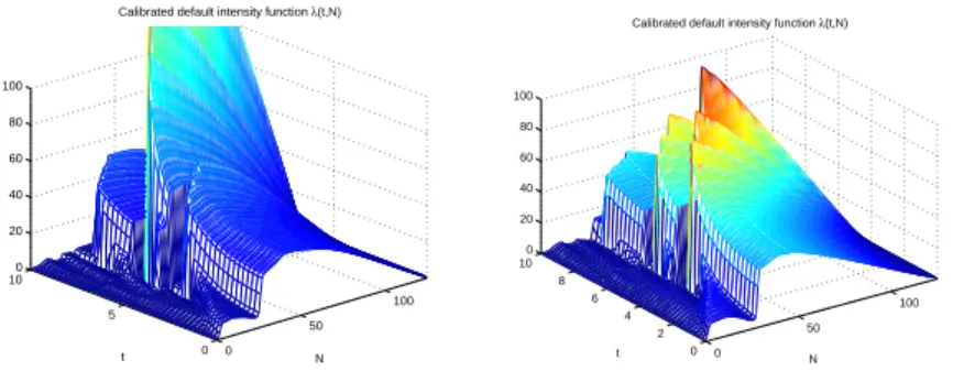
Figure 1: Model vs market spreads: ITRAXX September 26, 2005 (left) Sept 2008 (right). 0 50 100 0 5 10 0 20 40 60 80 100 N Calibrated default intensity function λ(t,N)

t 0 50 100 0 2 4 6 8 10 0 20 40 60 80 100 N Calibrated default intensity function λ(t,N)

t

Figure 2: Implied ITRAXX default intensity functions: September 2005 (left) vs Sept 2008 (right).

Figure 2 displays the local intensity function 𝜆(𝑡, 𝑙) as a function of time 𝑡 and the number of defaults 𝑙.

Several features deserve to be commented. First, we note the strong depen-dence of the default intensity on the portfolio loss level: as noted in section 3, this dependence is the signature of ’contagion effects’ in CDO tranches. Figure 2 shows the dependence of the default intensity with respect to the number of defaults at two different dates (in 2005 and 2008). We observe a similar pattern in both cases: while the initial default rate is quite low (less than 0.5, which means on average less one default every two years), this default intensity quickly increases as defaults occur in the portfolio, which is a clear signature of default contagion. Such contagion effects, which leads to the clustering of defaults, have been observed in historical time series [14]: our results indicated that their effect is also detectable in the implied default intensity, i.e. that contagion risk is effec-tively priced into market quotes of CDO tranches. In pricing terms, this steep initial slope means that in this period (2005-2007) equity tranches are priced

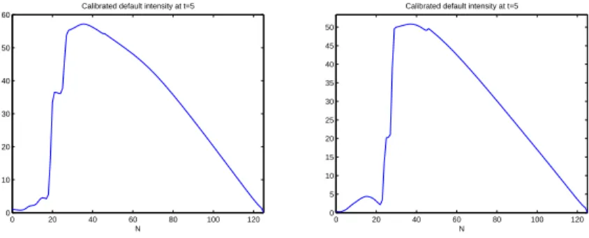
0 20 40 60 80 100 120 0 10 20 30 40 50 60 N Calibrated default intensity at t=5

0 20 40 60 80 100 120 0 5 10 15 20 25 30 35 40 45 50 N Calibrated default intensity at t=5

Figure 3: Implied default intensity as a function of number of defaults at a 2 year horizon: Sept 2005 (left) and Sept 2008 (right).

0 2 4 6 8 0 5 10 0 0.2 0.4 0.6 0.8 1 Number of defaults Years 0 2 4 6 8 10 12 0 0.1 0.2 0.3 0.4 0.5 0.6 0.7 0.8 Loss level Implied loss distributions

Figure 4: Left: term structure of loss distributions implied by ITRAXX Europe Series 6, March 15 2007. Right: loss distributions at various maturities.

relatively cheaply with respect to mezzanine or senior tranches. The values of 𝜆(𝑡, 𝑘) for small 𝑘 also give interesting insights for the pricing of first-to-default and 𝑘−th to default swaps.

Once the equity tranche of the portfolio is wiped out by defaults, we observe in figure 2 a plateau where the default intensity remains relatively insensitive to the number of defaults: in this regime,in fact, a constant, Poisson-type ap-proximation seems to work well. This regime corresponds to the bulk of the portfolio, composed of obligors whose default risk is well represented by the av-erage spread of the portfolio. From a pricing perspective, this flat region implied that, in these examples, apart from the equity tranche, the other tranches were priced assuming a constant (and high) value of the default intensity once the equity tranche has been wiped out. The steep decline of the 𝜆(𝑡, 𝑘) for large 𝑘 can be understood as corresponding to the group of obligors in the index with the lowest spreads/ default risk and which are the least exposed to systemic risk: they are the last to default, with a very low probability.

Finally we note that, as illustrated in Figures 1, 2 and 3, both the preci-sion of the calibration the qualitative features of the default intensity function remain the same throughout the period 2005-2008, a particularly turbulent pe-riod during which base correlations computed using Gaussian copula models have been notoriously unstable and sometimes impossible to calibrate to market spreads. This shows that the instability of such “default correlations” parame-ters is linked more to model mis-specification than to genuine non-stationarity: using a richer model structure along with a stable calibration algorithm restores a greater degree of parameter stability. This aspect is of course essential if the model is to be used for hedging [10].

We also note that there is a discontinuity in the dependence on 𝑡 at each observed maturity: this discontinuity is a structural feature related to properties of the dynamic programming equation and does not have any informational content . Such discontinuities are not present in quantities such as default probabilities (Figure 4).

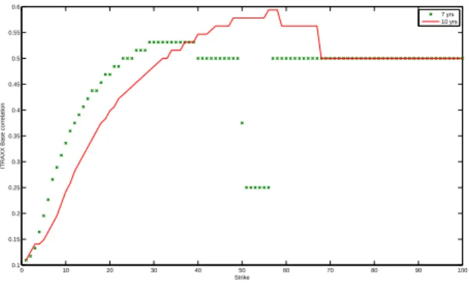
The above approach can be used to construct an arbitrage-free interpola-tion/extrapolation of ’base correlations’, by first calibrating the local intensity function to the observed tranche spreads then computing expected tranche losses for a fine grid of detachment points/maturities and converting them into a base correlation figure. Note that, unlike the usual linear interpolation of base lations, this method also provides an arbitrage-free extrapolation of base corre-lations beyond the largest detachment point and below the smallest attachment point. Figure 5 shows the result of such an interpolation for the ITRAXX data, compared with the linear interpolation method used by many market partici-pants. The difference between the two methods is striking, especially for senior tranches.

0 10 20 30 40 50 60 70 80 90 100 0.1 0.15 0.2 0.25 0.3 0.35 0.4 0.45 0.5 0.55 0.6 Strike

ITRAXX Base correlation

7 yrs 10 yrs

Figure 5: Base correlation surface generated by the calibrated model: ITRAXX Europe Series 6, March 15 2007.

6

Conclusion

We have proposed a rigorous methodology for calibrating a CDO pricing model to market data, by formulating the calibration problem as a relative entropy minimization problem under constraints and mapping it into an intensity control problem for a point process, which can be solved analytically.

By contrast with other calibration methods proposed for top-down CDO pricing models in the literature, our method proposed is nonparametric: it does not assume any arbitrary functional form for the default intensity. Another fea-ture of algorithm proposed is that it does not require preliminary interpolation or smoothing of CDO data in maturity or strike (which may violate arbitrage constraints), nor does it require a preliminary (model-dependent) “stripping” of CDO spreads into expected tranche notionals. In particular, our algorithm yields meaningful and stable results even for sparse data sets such as the ones available in CDS index markets.

Our method allows to compute portfolio default rates implied by index CDO quotes. Results obtained on ITRAXX tranche spreads point to default contagion effects in the riskneutral loss process and also illustrate that the implied default intensity corresponding to the first few defaults are very different from those of the bulk of the portfolio.

The model obtained from our calibration is a Markovian loss process where the default intensity depends on the current loss level and time. When compared with other possible specifications of top-down pricing models, the Markovian loss process considered here is of course quite simple in structure. Though it does account for clustering of defaults, it does not include, for instance, spread risk and the influence of other factors such as interest rates. Although more complex specifications are possible, as shown in Proposition 1, the information content

of CDO spreads does not allow to identify such models uniquely. Recently, Lopatin & Misirpashayev [26] have suggested to use a Markovian loss model as an intermediate step in the calibration of a two-factor model with richer dynamics using a relation such as (5) to link the parameters of the. In this context our algorithm can be used as the first phase of a calibration algorithm for a more complex model.

References

[1] Arnsdorff, M. and Halperin, I. (2008) BSLP: Markovian Bivariate Spread-Loss Model for Portfolio Credit Derivatives, Journal of Computational Fi-nance, 12, No. 2.

[2] Avellaneda, M. Friedman, C. Holmes, R and Samperi D. (1997) Calibrating the volatility surfaces via relative entropy minimization, Applied Mathemat-ical Finance Vol. 4, 37–64.

[3] Avellaneda, M. (1998) The minimum-entropy algorithm and related meth-ods for calibrating asset-pricing models, in: Proceedings of the International Congress of Mathematicians, (Berlin, 1998), Vol. III, Documenta Mathe-matica, 1998, pp. 545–563.

[4] Avellaneda, M., Buff, R., Friedman, C., Grandchamp, N., Kruk, L., and Newman, J. (2001) Weighted Monte Carlo: a new technique for calibrating asset-pricing models, Int. J. Theor. Appl. Finance, 4, pp. 91–119.

[5] Bismut, J.M. (1975) Contrˆole de processus de sauts, C.R. Acad´emie des Sciences Paris A281, 767–770.

[6] Br´emaud, P. (1981) Point Processes and Queues, New York: Springer. [7] Brigo D., Pallavicini A., Torresetti, R (2007) Calibration of CDO tranches

with the dynamic generalized Poisson loss model, working paper.

[8] R. Bruy`ere, R. Cont, R. Copinot, L. Fery, C. Jaeck, T. Spitz (2005) Credit derivatives and structured credit, Chichester: Wiley.

[9] Cont, R. and Tankov, P. (2004) Non-parametric calibration of jump-diffusion option pricing models, Journal of Computational Finance, 7, pp. 1–49.

[10] Cont, R. and Kan, Y. (2008) Dynamic hegding of portfolio credit deriva-tives, Financial Engineering Report No. 2008-08, Columbia University. [11] Cont, R. & Savescu, I. (2008) Forward equations for portfolio credit

deriva-tives, Chapter 11, in: Cont, R. (ed.): Frontiers in quantitative finance: credit risk and volatility modeling, Wiley.

[12] Cousin, A. & Laurent, J.P. (2008) An overview of factor models for pricing CDO tranches, in: Cont, R. (ed.): Frontiers in quantitative finance: credit risk and volatility modeling, Wiley.

[13] I. Csiszar (1967) Information-type measures of difference of probability distributions and indirect observation, Studia Sci. Math. Hungar, 2, 299318. [14] Das S., Duffie, D. and Kapadia, N. (2007) Common failings: how corporate defaults are correlated, Journal of Finance, Vol. 62, No. 1, (February 2007), pp 93-117.

[15] Ding X., K. Giesecke, and P. Tomecek (2006) Time-changed birth processes and multi-name credit, working paper.

[16] Duffie, D. and Garleanu, N. (2001) Risk and valuation of collateralized debt obligations, Financial Analysts Journal, Vol. 57, No. 1, (January/February 2001), pp. 41-59.

[17] B. Dupire (1994) Pricing with a smile, RISK, 7, pp. 18–20.

[18] Ekeland, I. and Temam, R. (1987) Convex analysis and variational prob-lems, SIAM.

[19] Errais, E., Giesecke, K., Goldberg, L. (2006) Pricing credit from the top down with affine point processes, Working Paper.

[20] Giesecke, K. and Kim, B. (2007) Estimating tranche spreads by loss process simulation, in: Hendersen et al. (eds.): Proceedings of the 2007 Winter Simulation Conference.

[21] Giesecke, K. (2008) Portfolio credit risk: top-down vs bottom-up, in: Cont, R. (ed.): Frontiers in Quantitative Finance: credit risk and volatility mod-eling, Wiley.

[22] Goll, T. and R¨uschendorf, L. (2002) Minimal distance martingale mea-sures and optimal portfolios consistent with observed market prices, in: Stochastic processes and related topics, 141–154, Stochastics Monographs, 12, Taylor & Francis, 2002.

[23] Gy¨ongy, I. (1986) Mimicking the one dimensional distributions of processes having an Ito differential, Probability theory and related fields, Vol. 71, No. 4, pp. 501-516.

[24] Lipton, A. and Rennie, A. (eds.): Credit correlation: life after copulas, World Scientific.

[25] Longstaff, F. and Rajan, A. (2008) An empirical analysis of the pricing of collateralized debt obligations, Journal of Finance, 63, 509-563.

[26] Misirpashayev, T. and Lopatin, A. (2007) Two-dimensional Markovian model for dynamics of aggregate credit loss, www.defaultrisk.com.

[27] R. Rouge and N. El Karoui (2000) Pricing via utility maximization and entropy, Mathematical Finance, 10, no. 2, 259-276.

[28] Sch¨onbucher, P. (2005) Portfolio losses and the term structure of loss transi-tion rates: a new methodology for the pricing of portfolio credit derivatives, Working paper.

[29] Sidenius J., Piterbarg V. and Andersen, L. (2008) A new framework for dynamic credit portfolio loss modeling, International Journal of Theoretical and Applied Finance, 11 (2), 163 – 197.

[30] Stutzer, M (1996) A simple nonparametric approach to derivative security valuation, Journal of Finance, 51, pp. 1633–1652.

[31] Zariphopoulou, Th. (2001) A solution approach to valuation with unhedge-able risks, Finance and Stochastics, 5, No. 1, 61–82.