EdVidParse: Detecting People and Content in
Educational Videos
by
Michele Pratusevich
S.B., Massachusetts Institute of Technology (2013)
Submitted to the Department of Electrical Engineering and Computer
Science
in partial fulfillment of the requirements for the degree of
Masters of Engineering in Computer Science and Engineering
at the
MASSACHUSETTS INSTITUTE OF TECHNOLOGY
June 2015
c
○ Michele Pratusevich, MMXV. All rights reserved.
The author hereby grants to MIT permission to reproduce and to
distribute publicly paper and electronic copies of this thesis document
in whole or in part in any medium now known or hereafter created.
Author . . . .
Department of Electrical Engineering and Computer Science
May 22, 2015
Certified by . . . .
Robert C. Miller
Professor, Department of Electrical Engineering and Computer Science
Thesis Supervisor
Certified by . . . .
Antonio Torralba
Associate Professor, Department of Electrical Engineering and
Computer Science
Thesis Supervisor
Accepted by . . . .
Albert Meyer
Chairman, Department Committee on Graduate Theses
EdVidParse: Detecting People and Content in Educational
Videos
by
Michele Pratusevich
Submitted to the Department of Electrical Engineering and Computer Science on May 22, 2015, in partial fulfillment of the
requirements for the degree of
Masters of Engineering in Computer Science and Engineering
Abstract
There are thousands of hours of educational content on the Internet, with services like edX, Coursera, Berkeley WebCasts, and others offering hundreds of courses to hundreds of thousands of learners. Consequently, researchers are interested in the ef-fectiveness of video learning. While educational videos vary, they share two common attributes: people and textual content. People are presenting content to learners in the form of text, graphs, charts, tables, and diagrams. With an annotation of people and textual content in an educational video, researchers can study the relationship between video learning and retention. This thesis presents EdVidParse, an automatic tool that takes an educational video and annotates it with bounding boxes around the people and textual content. EdVidParse uses internal features from deep convo-lutional neural networks to estimate the bounding boxes, achieving a 0.43 AP score on a test set. Three applications of EdVidParse, including identifying the video type, identifying people and textual content for interface design, and removing a person from a picture-in-picture video are presented. EdVidParse provides an easy interface for identifying people and textual content inside educational videos for use in video annotation, interface design, and video reconfiguration.
Thesis Supervisor: Robert C. Miller
Title: Professor, Department of Electrical Engineering and Computer Science Thesis Supervisor: Antonio Torralba
Title: Associate Professor, Department of Electrical Engineering and Computer Sci-ence
Acknowledgments
To those at MIT supporting my work: this work would not have been possible by the generosity of Rob Miller and the entire User Interface Design group at CSAIL -Carrie Cai, Juho Kim, Elena Glassman, and Max Goldman. They took me in when I was looking for a project and have been supportive ever since. Antonio Torralba and the Vision group also took me in and let me participate in some of the most innovative computer vision research happening at MIT. Thanks to Rebecca Krosnick for putting up with bad early prototypes. And thanks to Bryt Bradley for always smiling whenever I walk in the door.
To those who made MIT possible: thanks to my parents, Tatyana and Gennady, who encouraged me in the pursuits of my dreams, and have to put up with my taste for adventure. And of course, thanks to my ever-supporting boyfriend Robin, who is always a loving, snarky sounding board.
Contents
1 Introduction 6
2 Related work 8
2.1 Educational videos . . . 8
2.2 Object detection and scene recognition . . . 11
2.3 Convolutional neural networks (CNNs) . . . 14
2.3.1 AlexNet . . . 15 2.3.2 Improvements on AlexNet . . . 18 2.4 Evaluation metrics . . . 19 3 EdVidParse 23 3.1 System overview . . . 23 3.1.1 Design goals . . . 24 3.1.2 CNN feature extractor . . . 24 3.1.3 Feature processor . . . 26
3.1.4 Training and evaluating the bounding box estimator . . . 31
3.1.5 Potential improvements . . . 33
3.2 Advantage over R-CNN . . . 34
3.2.1 Using object proposals for bounding box estimation . . . 36
4 Applications 38 4.1 Classifying video production style . . . 38
4.1.2 An educational video dataset . . . 39
4.1.3 Results . . . 42
4.1.4 Discussion . . . 43
4.2 Extracting people and content for VideoDoc . . . 45
4.2.1 Problem . . . 45
4.2.2 Object annotation dataset . . . 46
4.2.3 Results . . . 47
4.2.4 Discussion . . . 47
4.3 Reconfiguring picture-in-picture videos . . . 51
4.3.1 Problem . . . 51
4.3.2 Results . . . 51
5 Discussion and Conclusion 54 5.1 Comparison of EdVidParse and R-CNN . . . 54
5.2 Conclusion . . . 55
Chapter 1
Introduction
Educational video content on the Internet is increasing at an exponential rate. In November 2014, 182 courses were offered on edX (edx.org), with over 1000 hours of video content. By June 2015, 516 courses were offered with over 6000 hours of video. Other massively open online course (MOOC) providers like Coursera (coursera.org) and Udacity (udacity.com) offer more than 1000 courses each at any given time. YouTube is the most common video hosting and distribution platform, with the recent YouTube EDU initiative hosting over 700,000 educational videos.
With this influx of content, researchers are interested in analyzing the effectiveness of video learning. This includes exploring the relationship between video composition and student engagement, and exploring alternate ways of presenting videos to learners at different stages of the learning process. For example, systems that effectively summarize videos or automatically extract slides can be beneficial for skimming or reviewing, while reconfiguring videos for fast playback can be good for initial viewing. While educational videos vary, most share two common attributes: people and textual content. People are presenting material, performing an experiment, and pro-viding a face to a new content. Textual content makes up the bulk of educational video material - graphs, tables, charts, images, formulas, and text present informa-tion. The composition of people and content in videos can give information about the type of video being watched. For example, if there is less textual content, the video is more likely about a topic from the humanities. Or if the size of the person
rela-tive to the rest of the frame is small, the video is more likely a classroom recording. Videos where a lecturer’s head features prominently are more engaging for learners [18]. Being able to effectively identify people and textual content in videos can be a useful tool in analyzing educational videos.
Computer vision techniques for analyzing images and videos have drastically im-proved in the last few years with the increasing use of neural networks, improving performance in vision tasks such as object detection and scene classification. The structure of an educational video is relatively consistent (when was the last time you saw a tropical beach scene in a traditional classroom recording?), so computer vision techniques specifically tuned for educational video applications can be effective.
This work develops a computer vision pipeline called EdVidParse for identifying people and regions of salient textual content inside a video. EdVidParse1 finds people
and textual content such as graphs, text, and drawings inside video frames. It also classifies the frame into a scene or composition type - for example whether it is a classroom-recorded lecture, a studio recording, or a synthetically-created image. These annotations allow researchers to answer questions related to the prevalence of people and textual content in educational videos. EdVidParse turns a video into a JSON annotation in near-real-time, taking about one second of processing per second of video. Alternative approaches to object detection in videos can be more accurate, but EdVidParse trades off some accuracy in exchange for speed.
This work also presents a dataset of object and composition annotations specif-ically in educational videos for training and testing models that achieved a mean average precision (AP) of 0.437 for object detection and 86 percent classification ac-curacy for scene classification. EdVidParse uses a new approach for training bounding box estimators using internal neural network features.
Three applications of EdVidParse are presented as case studies: automatically annotating videos by production style, detecting people and content bounding boxes for a textbook-like video interface, and reconfiguring a picture-in-picture video into a video of just slides.
1
Chapter 2
Related work
2.1
Educational videos
Because more students are learning online and through video, researchers are inter-ested in maximizing the effectiveness of these videos by exploring video composition, summarization, and content extraction techniques. Questions about which types of videos are more engaging, or how to make videos useful to learners after they have already been initially watched, are critical to increasing the effectiveness of online learning.
Guo et. al. [18] explores the relationship between video production style and student engagement. Videos from 4 courses were classified into 6 types of production styles, or composition: slides, code (a demo being worked through), Khan-style (for-mulas being incrementally derived without seeing a person), classroom (a recorded lecture video), studio, and office desk. The study classified each video into a particu-lar category, not taking into account videos that changed styles, say from a close-up of an instructor’s face to a Khan-style derivation. The researchers found that videos with high production value, namely shooting videos in a special video production stu-dio, did not result in greater student engagement and therefore might not be worth the money. The production styles proposed by Guo are a way of labeling a video in terms of composition, used as a foundation for the video style classification dis-cussed in Section 4.1. Having a system that can automatically classify each frame
of a video into a production style can allow faster data collection and more granular video analysis for engagement studies.
Eye-tracking studies with learners correlate learning with video frame content, with the goal of giving advice to content creators about effective video strategies. These studies show that it is easier for students to look at uncluttered text on a slide [35] and that students prefer watching videos with an instructor’s face, even if it does not increase recall of the material [25]. To perform these studies, each pixel of the frame needs to be labeled as belonging to a few groups, like person, background, or text material, and is usually done by drawing outlines of objects in the frame by the researcher. Having a technique that can automatically annotate objects to be manually fixed can save time for researchers performing further studies.
If classroom lectures are recorded and posted to the web, a problem is that lectur-ers often stand in front of relevant notes on a blackboard. While giving a classroom lecture, this is less of a problem, since students can ask for clarification when needed. However, this is not ideal in an online environment, where there is not the guarantee of a community that can answer questions. Instead of the lecturer changing their presentation style, alternate means of recording classroom lectures such as EduCase [20] present systems that work with the normal flow of classroom instruction. The EduCase system records an instructor in a classroom with multiple cameras and a depth sensor, automatically removing the lecturer from in front of the blackboard notes and reconfiguring the video to present both the lecturer and the notes in one video stream that is ready to post online. Being able to remove a lecturer from a video can make a recorded video more suitable for an online environment.
Because MOOCs are offered online to a massive audience, the data from student clicks, watches, rewinds, etc. provides an estimate of learner engagement with a particular video. Kim et. al. [23] aggregate student interaction data and correlate it with specific points in videos to understand why interaction peaks happen. For example, students tend to re-watch sections of video where the lecturer speaks too fast, or they tend to skip over longer boring sections. Being able to annotate more videos with video composition data can give more clues about the reasons behind
some interaction peaks.
Meanwhile, a goal of the Berkeley Video Digests system [32] is to provide an interface for effectively skimming a video or finding a point of interest. Much like chapter headings in books, Video Digests uses a combination of automatic, manual, and crowdsourced techniques to split an educational video into sections that can then be combined with a transcript in a skimmable format. Improving the automatic sectioning techniques can offer improvements for students reviewing material, since the current system does not take video composition into account.
Other crowd-sourced methods attempt to give section headings to video segments specifically in how-to videos [43]. These videos have a natural progression of steps, making it easier to verify with a crowd and offering natural breakpoints throughout the video. It is possible that clues within the video itself can offer a starting point for these section-level annotations.
In addition to summarization, the video watching interface can be combined with sectioning and transcripts to give the student a more granular view of a video, such as in the VideoDoc interface [28]. A lecturer can then design the video interface without the constraints of a single, linear experience by combining two potential video streams and lecture notes or transcripts in the same page. Sections are naturally broken up by video type, so a segment with a lecturer’s head might be followed by a segment with just a slide. Being able to automatically annotate textual content and lecturer’s head in the videos can save the lecturer work in splitting up the video view.
Another problem for learners with online videos is searching within a video for a relevant section. Text-based OCR solutions are common, using text displayed in the video as a description of what is happening inside the video itself. Yang et. al. [45] extract as much text as possible from the videos and apply OCR, so textual keywords can be used to search within a video. Yu et. al. [47] take this approach further to index an entire video with a set of keywords extracted from OCR on the intra-video text. While this approach works well for videos with high textual content, videos that rely on a lecturer speaking or doing a demonstration may benefit from visual cues within the videos. There is no way for a learner to search within a video based
on purely visual cues.
To solve the problem of video discovery, the Talkminer project [1] tries to aggregate educational videos into one search engine. Specifically, the focus is on extracting full-frame lecture slides from talks that are OCR’ed and indexed into a custom search engine. Users can then search for specific keywords that will return full videos around the desired slide to provide contextual information. The limitations are that videos with heavy blackboard work or slides that appear smaller in the frame are not indexed well.
Building further on the slide extraction idea, Wang et. al. [42] and Kayal et. al. [22] both take advantage of the similar structure in traditional lecture slides to further semantically extract information or build pages of notes from lectures. As lecturers become more innovative in their slide presentations, or even use them less frequently in their lecture videos, these approaches will be important for indexing previously-posted videos, and the techniques used by Wang and Kayal can be applied to videos with similar structure. However, a more general framework is needed for extracting content from general online educational videos.
Because researchers are interested in answering questions that relate to video structure, they can all benefit from being able to automatically annotate videos with areas of textual content and areas where people occur. These video annotations can help in answering questions about student engagement and help in designing interfaces for students interacting with videos.
2.2
Object detection and scene recognition
Parsing the visual structure of an educational video relies on a number of computer vi-sion techniques that were developed in literature in the more general case. Techniques have been developed to solve a variety of tasks with high speed and accuracy:
∙ object recognition - Classify an image of a single object into an object class, like dog, desk, book, etc. Features are first extracted from the image, then classified. Standard benchmarks include the ImageNet database [6].
∙ object detection - For an image, find bounding boxes around all instances of a given object class in that image. Standard benchmarks include the PASCAL database [11].
∙ scene recognition - Classify an image into a scene category, such as classroom, beach, office, etc. Standard benchmarks include the SUN database [44].
EdVidParse does both object detection and scene recognition - it detects peo-ple and textual content in videos, in addition to classifying video frames into video production style.
Hand-crafted features that rely on interest points in an image such as corners per-formed well at computer vision tasks until neural networks became popular. Features such as histograms of oriented gradients (HOG) [5] and SIFT [30] for static images and spatio-temporal features for video [26] perform well in ideal conditions, but are not robust to lighting changes, object occlusion, and viewpoint change. Part-based models attempt to account for these shortcomings by relying on a mix of parts for an object - so for example a person can be detected even if only his legs are seen. Scene recognition suffered the same shortcomings with the use of GIST features [31] - the features were not very robust to changes in viewpoint, lighting, or occlusion. Because educational videos are different enough in lighting and viewpoint, especially when trying to find people in the videos, more general features extracted from neural networks were used instead of hand-crafted features.
For object detection, an additional challenge is estimating the bounding box where an object occurs. Early approaches simply generated all possible image subregions and performed image classification on each region separately. A key improvement over exhaustive sliding-window search approaches was the idea of using non-maximal suppression to filter out high-scoring detections that significantly overlap previously-detected regions [13]. While this technique was originally used as part of a person classifier using part-based models, it is now generally used in all object detection tasks. EdVidParse relies heavily on object detection methods to find people and content effectively in video frames.
Instead of exhaustive enumeration of all possible object boxes, the idea of gener-ating a set of object proposals, or regions where there is a high probability of finding an object, were developed. An object proposal algorithm should have high recall -the correct detection should be in -the set of boxes it produces - but it can generate as many extra boxes as necessary, since classification will be performed on each object proposal anyway. Methods such as selective search [41] and edge boxes [50] are used to generate object proposals. These methods take advantage of the observation that a box with an object in it has a high density of edges inside the box. EdVidParse uses edge boxes and the associated code [7, 8, 50] for generating object proposals, notably in the R-CNN comparison described in Section 5.1.
For the classification step in all computer vision tasks, there are a number of available methods, with support vector machines (SVMs) being the most commonly used. SVM classification and training is done using the Liblinear (for linear kernels) and LibSVM (for other kernels) libraries [4, 12]. Typically grid search is used for finding a set of acceptable SVM parameters. This project uses the Spearmint1 package for hyperparameter selection, such as misclassification tolerance and bias [15, 36, 37, 38, 40]. Spearmint takes advantage of Bayesian optimization techniques to estimate optimal hyperparameters for a task, removing the need for arbitrary grid search for optimal parameters and decreasing training time. The best-performing algorithms on the PASCAL and SUN datasets use SVMs for classification, so EdVidParse uses this approach as well.
Another advantage of SVMs are that hard negative mining can be used to increase accuracy [13, 39]. In hard negative mining, an SVM classifier is initially trained with a dataset, then incrementally improved with negative examples. For example, say an SVM classifier is trained to identify whether the image is a dog or not. It is initially trained with 100 positive examples of dogs and 100 negative examples of dogs. To improve the accuracy of the classifier, thousands of random image crops from 1000 images known to not have any dogs in them are generated, and features are extracted from all those image crops. These negative examples are classified with the original
classifier, and those that are incorrectly classified are added as negative examples to the training set. This way, an initial classifier is incrementally improved only with negative examples it misclassifies.
Because EdVidParse is an object detection pipeline, techniques such as object proposals and classification with SVMs are key components to its effectiveness.
2.3
Convolutional neural networks (CNNs)
All the records set using hand-crafted features for computer vision tasks were over-taken by the use of convolutional neural nets (CNNs). The ImageNet Large-Scale Visual Recognition Challenge (ILSVRC) is an annual object recognition challenge where participants had to assign one of 1000 classes to a particular image of an ob-ject, and is often used as a performance benchmark for any new methods developed. In 2012, a team submitted an entry that beat all previous performance benchmarks in ILSVRC by nearly 20 percentage points, using convolutional neural networks as the basis for an object classifier [27]. Trained on more than a million images, this network learns more complex representations of images than was previously possible. The network architecture proposed in this 2012 ILSVRC entry became the standard in computer vision for any computer vision tasks and has been dubbed AlexNet. Since then, all winning entries in the ILSVRC have been CNN-based [34]. The basic principle of a convolutional neural network is that an image is fed through a series of learned convolutional filters layered on top of each other.
Network training end-to-end is achieved quickly using backpropagation [33] over millions of example images as training data. Additionally, the discovery and widespread use of rectified linear units (ReLUs) instead of sigmoid activation functions for neuron activations has led to better results at train and test time, according to Krizhevsky, et. al. [27]. Sigmoid activation functions, used in the neocognitron [14] (the precur-sor to neural networks) and in logistic regression classifiers, follow a sigmoid function, whereas ReLU activation functions look like a hockey stick, as shown in Figure 2-1. This means that when ReLUs are used, each individual activation is greater than
or equal to zero, with each positive value scaling linearly for that activation. This leads to more stability during training time, and the property that each neuron only lets through positive predictive values, rather than values that indicate absence. The use of ReLUs allows for the bounding box estimation procedure described in Section 3.1.3.
ReLU
Sigmoid
Figure 2-1: A comparison of the rectified linear unit (ReLU) and sigmoid activation functions
During training, because the errors from the training set are propagated through the network through back-propagation, this is called a backwards pass through the network. During the testing or feature extraction phase, an image is simply forward-passed through the network, performing the convolution and addition operations according to the learned parameters, but without propagating errors back through the network. EdVidParse takes advantage of fast forward passes through the network to extract features.
2.3.1
AlexNet
LeCun et. al. proposed using backpropagation and stochastic gradient descent in CNNs for hand-written digit recognition in the 1980s [29], and AlexNet built on these early ideas. But the success of CNNs until 2012 was mostly hindered by processing power and efficiency of training, so once this barrier was crossed, the effectiveness of using CNNs for vision tasks greatly increased.
AlexNet was so successful and revolutionary at the ILSVRC that the starting-point reference network architecture used by many research computer vision systems
exactly copies that of AlexNet. The network architecture is shown in Figure 2-2, and the sizes of the internal network outputs are shown in Table 2.1. Layers always take as input the output of the layers beneath them rather than the original image, so the resultant convolution can be complicated to understand. However, taking the result of a single 𝑛 × 𝑛 output in a given layer, called a unit, can provide insight about the contents of an image, as proposed by Zhou, et. al. [48], and discussed in Section 3.1.3. Each unit is composed of individual activations - responses of a particular activation to an image patch.
Figure 2-2: AlexNet neural network architecture used in feature extraction. Taken from Krizhevsky et. al. [27].
The three most common layer types in these neural networks are convolutional (conv) layers, pooling (pool) layers, and fully connected (fc) layers. A convolutional layer takes an image patch and performs a convolution on it according to some learned parameters. The resulting outputs taken together are the units for that network layer. For example, the conv1 layer outputs96 different units, all of size 55×55, computed by taking a series of convolution on image patches. Later convolutional layers perform the convolutions on activations of the units below them, not directly on an image patch. A pooling layer takes as input a number of activations and performs an operation on the activations to reduce the dimensionality. AlexNet uses max-pooling layers, which take as input the activations from the layer below it and outputs the maximum activation from the layer below. In this way, only the strongest activations are propagated forward through the network, reducing the number of parameters that need to be learned and the amount of data to be propagated through the system. Other types of pooling include average-pooling and min-pooling, but AlexNet uses
Layer Total output size No. of units Activations conv1 55 × 55 × 96 96 290400 pool1 27 × 27 × 96 96 69984 conv2 27 × 27 × 256 256 186624 2D units pool2 13 × 13 × 256 256 43264 conv3 13 × 13 × 384 384 64896 conv4 13 × 13 × 384 384 64896 conv5 13 × 13 × 256 256 43264 pool5 6 × 6 × 256 256 9216 1D units fc6 1 × 1 × 4096 4096 fc7 1 × 1 × 4096 4096 fc8 1 × 1 × 1000 1000 Total 1984 781736
Table 2.1: Output sizes of intermediate layers in the AlexNet reference network
max-pooling and this technique has become standard in deep network learning. Fully-connected layers simply compute a linear function as a result of their inputs, like in the neocognitron or linear logistic regression. The standard AlexNet architecture has 5 convolutional layers, 3 pooling layers, and 3 fully-connected layers. Typically, the output of the top layer in any network (fc8 in the case of AlexNet) is a vector of probabilities that perform the task the network was trained to do. In the case of AlexNet, the task was classification of an image into 1000 classes, so the fc8 layer has 1000 outputs representing the probability of belonging to each of these 1000 classes. The algorithm discussed for bounding box estimation in Section 3.1.3 takes advantage of the properties of each type of network layer.
The Caffe software [21] makes training, testing, and using neural networks efficient and easy. The standard AlexNet reference model, along with a number of other network models, are freely distributed online in the Caffe format, making development and testing straightforward. Because Caffe is open source, it is easy to distribute the final EdVidParse system online.
2.3.2
Improvements on AlexNet
After the success of AlexNet in the ILSVRC, CNNs were shown to be useful as general feature extractors [2, 9, 10, 46]. In general this is accomplished by passing an image through the network, and instead of looking at the output fc8 layer, the fc7 layer (which has 4096 output values) would effectively transform an image into a vector of 4096 values that can then be fed into any kind of classification, regression, or other system for tasks such as classification, bounding box estimation, image segmentation, and others.
As an extension to CNNs, the Region-CNN (R-CNN) algorithm was developed to be competitive at the object detection task. The basic idea is to use detected regions from an object proposal algorithm as inputs to the neural network, accomplishing both object detection and object recognition simultaneously [16]. The goal of the object proposal algorithm is to identify regions in an image that are likely to contain an object, reducing the task of exhaustive search using a set of heuristics.
It has also been shown that using a baseline network like AlexNet and fine-tuning it for a specific task such as scene recognition is effective and cuts down on train-ing time [17, 49]. The increase in performance from fine-tuntrain-ing AlexNet for scene recognition outperformed the previous record set the use of hand-crafted features, as shown by Zhou et. al. [49]. Zhou publicly distributes two networks - PlacesCNN and HybridplacesCNN, that have been fine-tuned from AlexNet for scene recognition and combined scene-object recognition respectively. Fine-tuning a neural network for a set of images or classes that it was not originally trained to do is called domain adaptation. In this work, fine-tuning was performed on a small set of scene-labeled images with the PlacesCNN network as a base [49], described in Section 4.1.4.
The biggest obstacles with using deep learning for computer vision tasks are the large amount of data needed for effective network training, long training times (often requiring multiple GPUs and complex CUDA code), and finding the optimal set of hyperparameters that govern learning. This work takes advantage of pre-trained networks that, when combined with a limited amount of training data for a specific
domain, can be used to achieve good results. Whenever possible, hyperparameters for learning rates and model selection were chosen based on parameters used by other researchers.
Recently, internal network units were shown to correlate with specific object de-tectors [48]. The main idea is that in networks trained for scene recognition, specific units act as object detectors, with the upper layers of the network synthesizing this information together to produce a final scene label. For example, in the PlacesCNN network, unit 3 in the conv5 layer activates in image regions containing faces. Because the main function of EdVidParse is detection of people and textual content (both are objects), this idea is used to find person and text units in deep networks. These units, most-studied in conv5 and pool5 layers, can be transformed into a mask on the image to serve as an estimator for object recognition. We heavily take advantage of this observation and develop a framework for constructing bounding box detection estimates using these internal features, detailed in Section 3.1.3.
2.4
Evaluation metrics
A number of metrics such as cross-validation accuracy, classification accuracy, pre-cision, recall, F1 score, and AP score, can be used to evaluate object detection and scene recognition metrics, each with costs and benefits. For evaluation in this work we choose to use classification accuracy for scene recognition and AP score for object detection.
Cross-validation accuracy is used primarily for classification or recognition tasks. In 𝑛-fold cross-validation, a training set is divided into 𝑛 groups, with each subset of 𝑛 −1 subgroups used for training and the last group used for testing. The cross-validation accuracy is the average of the correct classification percentage from all the test sets. With multiple classes, the mean cross-validation accuracy is the mean of all the cross-validation accuracies among all classes. This metric has the advantage that it gives a good estimate of test accuracy, since the hold-one-out approach simulates real data. Additionally, cross-validation can be a way of simulating more data, since
𝑛 −1 classifiers can be trained and averaged instead of 1. However, this metric does not take into account unbalanced training sets. For example, if a training set of 100 images only has 3 examples of class 𝐴 and 97 examples of class 𝐵, it is trivial to achieve 97 percent accuracy by always guessing class 𝐵 as the predicted label, no matter the train-test split. Even if the class labels were divided equally among training and testing splits, the high accuracy can be misleading.
Classification accuracy is simply a measure of the percentage of correct classifica-tions in a set of test labels. To combat class label imbalances, the test set should be equal in all class labels. This way a 75 percent classification accuracy for one class is comparable across all class labels.
Precision and recall can be used in evaluating object detection. For a given item in the test set, it is either a positive or negative example of a particular class 𝐶. A true positive is therefore an item in the test set that is both a member of 𝐶 and is identified as a member of 𝐶. A false positive is an item identified as class 𝐶 but is in fact not in class 𝐶. Precision is the ratio of true positives to true and false positives, measuring how good the false positive rate is:
precision= true positives
true positives+ false positives (2.1) If a detection system achieves 100 percent precision (or a precision of 1), it means that all the objects identified as class 𝐶 are in fact of class 𝐶, but it is not guaranteed that all objects of class 𝐶 were found.
By contrast, recall is the ratio of true positives to true positives and false negatives, measuring the retrieval rate of the algorithm:
recall= true positives
true positives+ false negatives (2.2) An algorithm with 100 percent recall (or a recall of 1) finds all instances of class 𝐶, but is not guaranteed to find only those items. To trivially achieve 100 percent recall, all possible items are identified as members of class 𝐶.
recall, the harmonic mean of precision and recall, or the F1 score can be used:
F1 = 2 · precision · recall
precision+ recall (2.3)
However, the drawback of this metric is that F1 only takes into account a specific value of precision and recall - rather than the relationship of precision and recall at different values. At 100 percent recall, there might only be 20 percent precision. But at 50 percent precision there can be 100 percent recall. Because there is a specific relationship between precision and recall, it makes sense to use a metric that takes into account all pairs of precision and recall values.
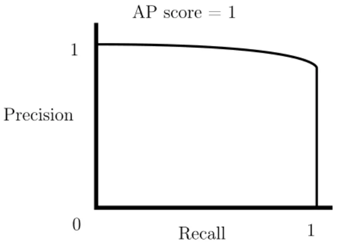
0 1 AP score = 1 Recall Precision 1
Figure 2-3: An ideal precision-recall curve with AP = 1
The AP score (or average precision) of a detector takes into account the relation-ship between precision and recall. Average precision is defined as the area under the precision-recall curve. An ideal detector has an AP score of 1, with a precision-recall curve like shown in Figure 2-3. This curve is calculated by ordering the predicted results by highest confidence and their corresponding correct labels, thresholding at various values, and plotting the precision and recall at those thresholds. The more that a precision-recall curve looks like this ideal, the better the detector. Instead of looking at the precision-recall graph to determine effectiveness, the AP score is used. The AP score metric has the advantage of taking into account all points on the precision-recall curve.
meaning as for one-class classification problems. To extend the AP score metric to multiclass problems, the AP score for each class separately is averaged to compute a mean AP score for the detector.
For scene recognition, test set accuracy is used, as is standard for multiclass clas-sification problems. For object detection, AP score is used for both model selection and final evaluation [24]. This is consistent with the metrics used in computer vision literature for both classification and object detection.
Chapter 3
EdVidParse
3.1
System overview
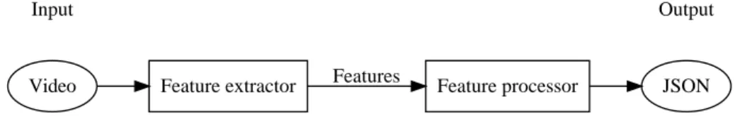
EdVidParse is composed of two main pieces - the feature extractor and the feature processor. The feature extractor turns a video into a set of numerical features, and the feature processor either performs classification or bounding box estimation and outputs computer-readable JSON.
Feature extractor Features Feature processor JSON
Input Output
Video
Figure 3-1: High-level system diagram for the video parsing tool
EdVidParse is written in Python, making it easy to quickly make changes to any part of the pipeline. The feature extractor that uses neural networks uses the open-source Caffe library [21] for efficient feature extraction and for ease of development. The feature processor uses the Liblinear and LibSVM libraries for classification [4, 12], and a custom-written interface for bounding box estimation.
There are two main tasks EdVidParse can accomplish - classification of a video frame into a style, such as pure slide, picture-in-picture, classroom lecture, etc., and detection of people and textual content in a video frame.
3.1.1
Design goals
EdVidParse has three main design goals:
∙ Accuracy - EdVidParse must be accurate enough to require minimal manual adjustment. Without working fast, there is no reason for a researcher to use a tool that accomplishes the same task that can be done more accurately by hand.
∙ Speed - Small accuracy tradeoffs in exchange for speed are acceptable. For a tool to be used, it must work reliably enough to need only minor manual adjustments.
∙ Trainability - A tool that can be re-trained with new video data will be more robust to changes in the future.
3.1.2
CNN feature extractor
The purpose of the feature extractor is to decompose the input video into frames, then extract image features from each of those frames (see Figure 3-2). While all video frames can be extracted from a video, in practice approximately one in every five frames are used for feature extraction. This is because adjacent frames in high-frame-rate videos do not change appreciably, but can instead cause noisy results later in the pipeline.
Feature extractor
Frames
Image transform Fill? Crop? Warp?
Mean subtract BGR format
Network forward pass AlexNet? HybridplacesCNN?
PlacesCNN?
Features Video
Figure 3-2: System diagram for feature extractor
Before the image is sent through the network, it goes through a pre-processing step where the image is converted from RGB-space to BGR-space and resized to227 × 227
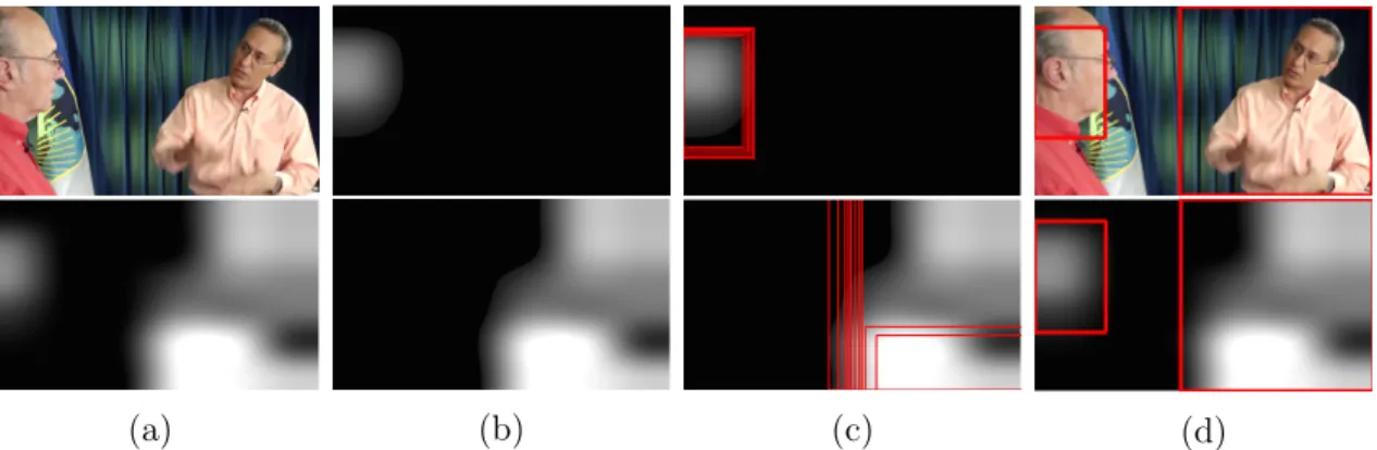
pixels, since this is the input type AlexNet requires. Additionally, the training image mean (a standard image distributed with AlexNet) is subtracted. When images are not square, there is a choice of cropping, filling, or warping the images to transform them to 227 × 227. Cropping finds the largest centered square piece of the image and scales it to the appropriate size. Filling scales the image as-is so that the largest dimension fits, then fills in the rest of the space with black pixels. Warping just resizes the image without any cropping or filling. Filling and cropping preserves in-image ratios, but objects appear smaller and can be harder to detect. Warping utilizes the entirety of both the original image and the final227 × 227 area. Figure 3-3 shows the difference between the three pre-processing methods. Generally, the method chosen is warping, as standard with the original AlexNet, except in specific situations, as discussed in Section 3.2. With every rescaling operation there is a choice with the kind of pixel interpolation to use - nearest neighbor, bilinear, bicubic, etc. A good compromise between speed and accuracy that is used in the literature is generally bilinear interpolation [16], except in the specific case described in Section 3.1.4.
(a) Original image, 1280 × 720 pixels
(b) Fill, 227 × 227 pixels (c) Crop, 227 × 227 pixels (d) Warp, 227 × 227 pixels Figure 3-3: Difference between cropping, filling, and warping in the image pre-processing step. Filling and cropping preserves in-image ratios, but objects appear smaller.
Network activations are calculated using one of four networks, depending on the task. These are the standard AlexNet distributed with Caffe [21], PlacesCNN [49], HybridPlacesCNN [49], and a custom network fine-tuned from Places (described in Section 4.1.4). The feature extractor does a forward-pass of each frame, saving the activations from all layers of the network. All these features are passed to the feature processor. A choice in model selection is which network features to use. PlacesCNN is tuned with scenes rather than objects, so we expect PlacesCNN to perform better than AlexNet or HybridplacesCNN when looking for bounding box estimations, according to recent work in object detection from scene prediction [48]. So in the model selection stage, multiple networks are tried and the best one is used in practice.
3.1.3
Feature processor
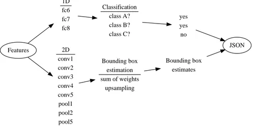
Features 1D fc6 fc7 fc8 2D conv1 conv2 conv3 conv4 conv5 pool1 pool2 pool5 Classification class A? class B? class C? Bounding box estimation sum of weights upsampling yes yes no JSON Bounding box estimatesFigure 3-4: System diagram for feature processor
The extracted features from a network forward-pass are either one-dimensional or two-dimensional. From the architecture of AlexNet described in Figure 2.1 and Table 2.1, passing an image through the network in a forward pass results in over 10000 unit activations (and over 750000 individual activations) in 11 different layers of the network. Two kinds of features emerge: (1) one-dimensional feature vectors, such as fc6, fc7, and fc8, which are numerical image descriptors of the entire image, and (2) 2-dimensional units, such as a single set of activations for a specific convolutional or
pooling layer output. The one-dimensional feature vectors are used for classification, and the two-dimensional units are used for bounding box estimation. See Figure 3-4 for a summary of the feature processor.
Classification, or feature processing from 1D feature vectors
The one-dimensional feature vectors are input into a trained SVM classifier that can classify an entire image into a particular scene category. SVMs are used for ease of use and training. In model selection, 10-fold cross-validation accuracy was used to determine the best features and SVM parameters to use. The accuracy of the video production style classifier is discussed in Section 4.1.3.
Mask generation from 2D units
The 2D units are used to generate a rectangular bounding box estimate from an image. Each unit can be a mask over the entire image, based on the values in the unit activations. Figure 3-5 shows an example of an image and the masks that are generated through various operations on a specific unit. To generate a mask 𝑃 from one unit, the unit is preprocessed in the opposite way that the image was preprocessed before going into the network. In the simplest case, if the image was warped before being passed through the network, the unit is upsampled and rescaled to the size of the original image. If the image was initially filled then scaled, then the activation must be scaled then un-filled (in other words, cropped). Because the goal is to estimate a rectangular bounding box, nearest-neighbor estimation is used. In addition to inverse preprocessing, the unit is thresholded, either before or after the upsampling. The thresholding operation can be intuitively thought of as a filtering operation -while the unit activations may contain all the true positive activations, they will have small false positive activations that are amplified during the upsampling process, and thresholding filters out potential false positives. The EdVidParse pipeline thresholds after upsampling to avoid nonlinear optimization during training. A 2D unit is used to generate an image mask that can then be used for bounding box estimation.
(a) Original image
(b) Nearest neighbor interpo-lation, no thresholding
(c) Thresholding, then near-est neighbor interpolation
(d) Nearest neighbor interpo-lation, then thresholding
(e) Bilinear interpolation, no thresholding
(f) Thresholding, then bilin-ear interpolation
(g) Bilinear interpolation, then thresholding
Figure 3-5: A single unit serves as a mask on the original image. If the unit is trained to recognize specific objects, the mask can give hints about where the object is located. An image and the interpolated activations from unit number 138 in the pool5 layer of the Places network is shown.
of a particular unit in conv5 known to have high activations for faces. The activations are shown with a few options for interpolation and thresholding. Nearest neighbor interpolation and thresholding are commutative operations, whereas bilinear interpo-lation and thresholding are not.
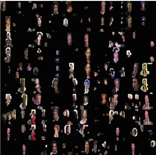
Generating masks from the same unit activations over many images, it is com-pelling that specific units activate to specific objects [48]. For example, as shown in Figure 3-6, looking at the activations from unit 3 in the pool5 layer, it is clear that this particular unit responds well to faces. More unit visualizations are shown in Appendix A.
The examples shown in Figures 3-5 and 3-6 are masks generated from a single unit, but multiple units can be used for more accurate estimation. Single-unit
acti-Figure 3-6: Activations from unit number 3 from the conv5 layer using the Places network over 100 images in the educational video dataset.
vations, most often from pool5, have been studied as features to use out-of-the-box for classification or regression tasks, as discussed in Section 2.3.2. However, we claim that using a linear combination of unit activations will achieve better domain adap-tation for object classes not in the original network training set, as in the case of educational videos. In other words, a prediction mask 𝑃 is calculated from a subset of unit activations by
𝑃 = 𝑊 𝐹 = ∑︁
𝑓 ∈ units
(𝑤𝑓𝑓), sparse 𝑊 (3.1)
where 𝑓 is a single 2D unit activation and 𝑤𝑓 is a scaling weight for all activations
in that unit. The weights are learned for each specific object class, as described in Section 4.2. Sparse weights are desired because it reduces overfitting of the units
in addition to reducing computation. The mask 𝑃 is fed into the bounding box estimator.
EdVidParse uses a single threshold on 𝑃 rather than thresholding each individual unit 𝑓 . An extension of this project using non-linear optimization techniques to learn individual unit thresholds can potentially produce better results.
Bounding box estimation from an activation mask
An activation mask is turned into a bounding box estimate for an object with a series of thresholding and estimation operations.
(a) (b) (c) (d)
Figure 3-7: Turning an activation mask 𝑃 into a bounding box. (a) The original image is turned into a thresholded activation mask. (b) The mask is split into connected compo-nents. (c) Multiple boxes are generated from each connected component. (d) Non-maximal suppression is applied to find only the best boxes.
After calculating an activation mask 𝑃 for a particular object class, 𝑃 is thresh-olded and split into connected components. For each connected component, a number of bounding boxes are generated and a score is calculated for each box around the activations of that connected component. Then, on the boxes generated for the en-tire image, non-maximal suppression is performed to give an optimal set of bounding boxes for the object in question. An example of taking an activation mask and turn-ing it into a boundturn-ing box is shown in Figure 3-7. The threshold parameters are learned based on the detection task, such as the person and content detection task described in Section 4.2. To find the optimal noise-removal threshold, the mask 𝑃 is subject to multiple thresholds, and connected components are calculated for each threshold.
The score 𝑆 for each box is the ratio between the average activation in the box and the average activation in the image, shown in Equation 3.2. Non-maximal suppression is then performed on all boxes at all thresholds with scores 𝑆.
𝑆 = ∑︁ 𝑎∈box 𝑎 ∑︁ 𝑎∈image 𝑎 ·area of image area of box (3.2)
The highest-scoring bounding boxes above a score threshold are the bounding box estimates for that object class.
3.1.4
Training and evaluating the bounding box estimator
The bounding box estimator does simultaneous detection and classification of a given object class. The idea is to train the estimator with a small number of bounding-box-annotated images of a particular class and rely on the internal network representation of the image to generate the bounding box.
A training set annotated with ground-truth bounding boxes for people and content is converted into binary masks of size 55 × 55 (because this is the size of the largest unit from conv1). An image without a positive example of the class is all black. These binary ideal activation masks flattened into a matrix are the ground truth activations 𝐺. In an ideal world, they are the activations we would like to generate through a linear combination of unit activations, which would map exactly to the bounding boxes we want to generate. Because of the ReLU units used in each neural network layer, the unit activations will have only positive values, meaning that an image without a positive example will be returned all black from the network, mirroring our training data.
All the training images are then passed through the network, and all the internal unit activations are resized to 55 × 55 using nearest-neighbor interpolation to create the unit matrix 𝐹 .
We then learn a set of weights 𝑊 to minimize the pixel-level L2 error 𝐸 over all images in the training set, shown in Equation 3.3. We want to L1-regularize the 𝑊
matrix to rely on a sparse set of units 𝐹 . 𝐸 = ∑︁ images ∑︁ pixels (𝐺 − 𝑊 𝐹 )2 (3.3)
However, there is a practical limitation to computing this matrix 𝑊 in its entirety. With a training set of merely 50 images, all the activations in the 2D units scaled to equal size of 55 × 55 to construct the 𝐹 matrix will take approximately 2.5 GB to store in memory, assuming a float takes8 bytes of memory.1 This poses a problem for
finding an exact sparse solution of unit weights 𝑊 , because the least-squares solution requires computing 𝐹𝑇𝐹 , or having two copies of 𝐹 in memory simultaneously.
Instead, we propose a greedy algorithm that takes advantage of the simultaneous optimizations we would like to do. First, iterate through all the units, solving the least squares problem in Equation 3.3 with each unit one by one to find the unit that yields minimum error. Then, for as many units as desired, iterate through the units to solve the least squares solution for the growing list of best-fit units. The advantage of this algorithm for finding optimal units is that it iteratively builds the units that best complement one another. If a particular unit is chosen because it provides the smallest error when it stands alone, the next maps are chosen specifically based on the performance of the first. No assumptions are made about the weights - they do not have to be positive. Negative weights imply that the activations of a particular unit provide a negative estimate about the presence of the particular object class. In practice, all the weights that are computed by this method are positive, implying that the algorithm learns to construct positive activations rather than deconstruct negative activations.
Once the weights 𝑊 are learned, the bounding box is estimated as described in Section 3.1.3. Model selection is performed on how many units to use, which features to use to extract the unit activations, and the final thresholding operation. A bounding box can be extracted with weights and a threshold learned from this method in under one second on a CPU, since only a single forward-pass through the
network is required.
One potential limitation to this greedy approach is that it is possible to find a set of units that work better together than separately. For example, the first unit found by the algorithm minimizes the pixel-level error, but it is possible that the two units that would minimize the pixel-level error do not contain the first found unit. To combat this and provide regularization with our training data, once the final units are found, we train the weights using L1 regularization to ensure sparsity. It is not guaranteed that a single unit will work for bounding box estimation, and in practice the best performance occurs with 2 or 3 units.
3.1.5
Potential improvements
One limitation of the algorithm in its current state is that the algorithm does not take into account the “random noise” responses of its activations. A given unit responds with high activation to the image region that contains the object of interest, but it also responds to other parts of the image with some small activations that can effectively be considered noise. To account for this, we choose to learn a single threshold at the end of the linear combination to filter out this activation noise. However, in practice this is not as effective as thresholding a single set of unit activations before the weights are learned. If a set of thresholds and weights is learned simultaneously for the units, the problem becomes a non-linear optimization problem that is hard or impossible to solve by analytical means. Early experiments with learning unit weights yielded thresholds that were close to zero, so this work lays does not attempt to learn a set of thresholds for each unit. More experiments are needed to determine whether this non-linear optimization will prove more effective than the results given here.
An additional step that might offer improvement is learning a bounding box re-gression algorithm that takes as input the bounding box from the estimator and regressing to a bounding box that is potentially more correct, like the approach taken by Girshick et. al. [16].
3.2
Advantage over R-CNN
There are a number of downsides to using R-CNN, the existing method for object detection using deep features [16], and EdVidParse improves on these disadvantages. The effectiveness of R-CNN strongly depends on the image preprocessing step, there are many parameters to tune, the method is very slow at train and test times, and there no information about the internal image representation is used in prediction. However, an advantage is that R-CNN can be very accurate. EdVidParse is invariant to preprocessing, has few parameters, is fast to train and test, and uses internal network representations for prediction.
The R-CNN pipeline involves generating object proposals for a given image (typi-cally1000 or more), preprocessing that image region, extracting fc7 features from the network, and classifying the image region with an SVM for each object class. During training, thousands of object proposals are generated, sent through a network, and used to train the SVM with hard negative mining. In contract, EdVidParse takes unit activations from a single forward-pass in the network and constructs a bounding box from the unit activations.
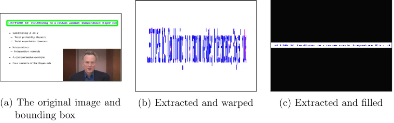
In R-CNN, the choice of image preprocessing greatly affects the outcome of the classification. If a proposed image crop is highly non-square, simply warping the crop will produce an image that is also hard for humans to identify. In the example of detecting people and content in educational videos, this is especially a problem, as shown in Figure 3-8. The fc7 features extracted from these image patches will be different enough that a classifier trained on these images will not be invariant to all kinds of preprocessing. EdVidParse on the other hand, because it depends on internal network representations, is invariant to image pre-processing.
Additionally, in R-CNN training there are many parameters to tune - each set of SVM parameters in addition to the object proposal algorithm parameters (of which there can be 10s of parameters), the hard negative mining parameters, and oth-ers. Training R-CNN end-to-end with Bayesian optimization is not an option, since training the entire system takes too long and Bayesian optimization shows limited
(a) The original image and bounding box
(b) Extracted and warped (c) Extracted and filled
Figure 3-8: An example of an image region that, when sent through the R-CNN with simple warping, will not yield good results. In this case, cropping and filling will yield similar results because the bounding box is highly rectangular.
improvement over grid search for large sets of parameters. In our comparison ex-periments between our proposed algorithm and R-CNNs we train each piece of the R-CNN pipeline separately, like the original authors. By contrast, EdVidParse has a small number of parameters that can be trained end-to-end.
Finding object detections in a single video frame for R-CNN is very slow. With 1000 or more object proposals to generate for each frame, each one has to be resized and interpolated for network processing, passed through the network, then ranked and sorted to perform non-maximal suppression. This results in around 1000 forward-passes through the network, one for each object proposal. In EdVidParse, only a single forward-pass is needed, decreasing the processing time by a factor of 100 or more.
R-CNNs do not take advantage of any of the internal network representations of the images in the network. It only relies on fc7 features, which do not have any physi-cal meaning for the image, discarding any unit activations from lower in the network. In contrast, EdVidParse takes advantage of the internal network representations and does not discard information.
However, a distinct advantage of R-CNNs is the ability to train the final SVM with hard negative mining, with as many examples as needed to get the desired performance. With the almost exhaustive list of object proposals, the AP score achieved with R-CNNs can be as high as 0.90 depending on the training set. When high accuracy is desired and speed is not an issue, R-CNNs prove a valuable tool for
object detection. Because one of the design goals of EdVidParse was speed, using internal feature representations was much faster than using R-CNN.
3.2.1
Using object proposals for bounding box estimation
EdVidParse generates bounding boxes around objects, but does not benefit from using an object proposal algorithm before bounding box estimation. The edge boxes object proposal algorithm used in R-CNNs is extremely fast and highly tunable [50]. For a given set of training images annotated with object bounding boxes, the parameters are tunable to achieve high recall for that object class.
The object proposal algorithm used in comparisons of R-CNN and EdVidParse is the edge boxes algorithm described by Zitnick, et. al. [7, 8, 50]. The basic idea of the edge box algorithm is that objects in an image have certain edge properties. For example, an object generally has a large cluster of complete edges inside a square region. According to some tunable parameters, such as how far apart to sample boxes across the image, the edge boxes algorithm can be tuned for images of particular sizes or images that have particular objects. An example of using object proposals with EdVidParse is described in Section 4.3 about reconfiguring picture-in-picture images. To combine object proposals and bounding box estimation, generate a set of object proposals and assign each box a score according to the formula given in Equation 3.1. This can solve the problem of how to generate bounding boxes from the unit activations as described in Section 3.1.3. However, the downside to this approach is that the bounding boxes that get generated in the final image are then limited to the bounding boxes proposed by the edge boxes method. Zitnick et. al. claim that on the PASCAL dataset, 96 percent recall is achieved with an acceptable overlap tolerance of 0.5, and 75 percent with the stricter overlap tolerance of 0.7 [50]. This means that the success of the overall bounding box estimator is dependent on the object proposal estimator, since the recall is not 100 percent.
In our experiments, we achieved worse recall rates for classes that did not originally appear in the PASCAL training set, namely for text content. Using object proposals and assigning scores to them using the bounding box estimator method yielded worse
results across all classes compared to not using them, and this is probably because the success of the final estimation is limited by the object proposals and therefore by that algorithm. However, Section 4.3 gives an example of a use case where, because of strong priors on the kinds of boxes we want to generate, using edge boxes can guarantee increased performance.
Chapter 4
Applications
This section will describe three case studies for using EdVidParse to do three tasks related to educational videos: (1) classifying videos by production style, (2) generating bounding box predictions for people and content, and (3) reconfiguring a picture-in-picture video.
4.1
Classifying video production style
4.1.1
Problem
Videos in online courses come in many different styles, and EdVidParse can answer questions related to video style. For example, some videos are filmed in a production studio with an instructor lecturing at a podium, and others are classroom lecture recordings cut into pieces and posted online. Sometimes an instructor’s face features prominently, other times the video is a presentation with a voiceover. Some videos even vary style mid-video, for example from classroom recording to a close-up of a slide. Researchers are interested in questions like whether high production value videos or the presence of a lecturer in a frame increased student engagement.
In the study by Guo et. al. [18], the question is the correlation between video production style and student engagement. For this study, researchers used a number of videos from four computer science courses on edX, and gave each video a single
production label. The conclusions from the study were that high production cost videos do not increase student engagement. However, EdVidParse can offer greater insight into this question, since it can classify videos into categories on a more granular level, giving a label to each frame.
EdVidParse classifies each frame in an educational video into one or none of 9 labels described in Table 4.1 using an SVM classifier on top of fc7 features with a test set accuracy of 86 percent. To accomplish this task, a hand-labeled dataset was used for training and testing.
4.1.2
An educational video dataset
Data collection
A set of educational videos was collected and annotated for training and testing. Educational videos are available free of charge from edX for registered course users. To take advantage of this, an automated script using Selenium [3] auto-registered for all of the courses offered on edX in September 2014 and scraped the pages for all links to videos hosted on YouTube. A total of 6914 video URLs were collected from 181 courses from varied disciplines.
0 10 20 30 40 50 60 Length (mins) 0 200 400 600 800 1000 1200 1400 F requency
Histogram of video lengths
Figure 4-1: Histogram of video lengths from the scraped edX videos
Because all the edX videos are hosted on YouTube, basic information about the videos, such as length and frame rate, can be accessed via the YouTube API. Figure
4-1 shows the distribution of video lengths of the videos scraped from edX, where the average video length was9.11 minutes, consistent with the findings from Guo’s study. Nearly all videos had a frame rate of 30 frames per second (fps), so they were very high quality.
To create a dataset, 1600 frames were randomly selected. First, 800 URLs were randomly selected from the scraped list. Then, from each video, two random times were selected. Each frame was labeled with both a scene label and with object annotations. Any frame that was all black or that was a fading transition between two types of frames was rejected from the dataset. In total, 1401 images were split into a training set and testing set. The test set has 20 images from each class label, and the rest of the images make up the training set.
Scene annotations
Scene annotations are assigned labels from a semantic understanding of the world. Humans are able to identify a dining room, despite there not being a standard dining room template. While there are visual similarities between scene types, there are even more differences. This idea can be applied to frames from educational videos, giving each extracted frame a single label describing the type of scene in the frame.
The scene labels used for this dataset were a modified list taken from Guo’s study. A full list of scene labels together with a description is shown in Table 4.1. The office label assigned by Guo was renamed head to make it more general. To accommodate various styles of videos and single them out specifically, more categories were added, such as picture-in-picture (abbreviated to pip), synthetic, and discussion, that were not specifically mentioned by Guo because those types of videos were not common in computer science courses that were the focus of the study. Examples of each kind of scene label are shown in 4-2, and a frequency histogram for each label is shown in Figure 4-3. Because of the imbalance in class frequencies, the test set contains 20 examples of each class label, so test set accuracy and the confusion matrix are reported for accuracy. When some categories had limited data, videos were found manually for more examples to ensure at least 50 examples per class.
Scene labels Description
code A software demo or full-screen code-writing in an IDE discussion Multiple people in a frame talking
Khan-style Free drawing on a tablet or paper, in the style of videos popularized by Khan Academy
talking head Mostly contains the instructor lecture From a live classroom recording
picture-in-picture Slide with a square overlay of an instructor in a corner slide PowerPoint-like slide presentation, just with educational
content, sometimes containing just images
studio Staged recording of an instructor in a studio with no audience synthetic An instructor and an overlay of slide content, but not in
rigid format like picture-in-picture
Table 4.1: Scene label categorization description
(a) code (b) discussion (c) Khan-style
(d) talking head (e) lecture (f) picture-in-picture
(g) slide (h) studio (i) synthetic
Figure 4-2: Example frames for scene labels
Labels were chosen in an attempt to minimize ambiguity using their original se-mantic definitions. For example, a frame that contained a full-frame picture of a famous person was classified as slide rather than head since it represented slide con-tent presented to a leader, and slides that a person drew on to progressively explain
code
discussion head khan-style lecture pip slide studio synthetic Scene label 0 100 200 300 400 F requency 62 145 430 55 125 62 401 52 104
Histogram of scene labels
Figure 4-3: Frequency histograms for scene labels in the educational video dataset
concepts was labeled as Khan-style.
4.1.3
Results
The overall test set accuracy is 86 percent classification accuracy. Each class SVM is trained separately, then used together for test classification. Table 4.2 gives the confusion matrix for the classifier, showing that the classifier more likely doesn’t classify an object into a category rather than confusing two categories.
Each class is trained with a separate linear kernel SVM. The best model for each class was chosen based on which combination of fc7 features (AlexNet, Hybrid-placesCNN, PlacesCNN) and SVM parameters (L1 / L2 regularization, C value, bias) had the highest 10-fold cross-validation accuracy on the combined training and valida-tion sets. All images were warped for classificavalida-tion, because this is how the networks were trained. Gaussian kernel SVMs are not used in training to avoid overfitting. A Gaussian kernel exploits nonlinear relationships between the data points and can find separating planes between the data when there are none, so to avoid overfitting on the limited training data, Gaussian kernels were not used.
Predicted label
code discussion head khan-style lectur e
pip slide studio synthetic other
code 0.75 0.25 discussion 0.95 0.05 head 0.95 0.05 khan-style 0.75 0.25 True lecture 0.85 0.15 label pip 0.75 0.25 slide 0.95 0.05 studio 0.85 0.15 synthetic 0.95 0.05
Table 4.2: Confusion matrix for video production style classification
one class label based on which decision value is greatest. For example, an image can get an SVM score of 0.95 from label 1 and 1.35 from label 2, so even though the image was given a positive score by two models, it will be assigned label 2 because the decision value is greater. An image with no positive classifications is not given a label, so it is classified as other.
4.1.4
Discussion
The overall test set accuracy is 86 percent on the held-out test set, and the confu-sion matrix is given in Table 4.2. EdVidParse is more likely to not classify a label at all than confuse that label with another class. The classes that are hardest for EdVidParse to classify are the code, Khan-style, and picture-in-picture classes, which do not get classified correctly 25 percent of the time. Overall the classifier performs well when presented with many different kinds of images, especially on the discussion and head labels, since they are very distinct visual categories.
Despite the visual similarity between code and slide frames, the classifier can dis-tinguish between the two types well, more likely not assigning a label at all rather than incorrectly classifying the frame. There are no classes that are commonly con-fused by the classifier, and the most common failure more in general is that a given frame is not classified into any category rather than being incorrectly classified.