Diving Deep into the Determinants of Driver Dwell
byMichelle Catherine Roy
Bachelor of Business Administration in Supply Chain Management, Texas A&M University, 2016 and
Leora Reyhan Sauter
Bachelor of Science in International Relations, United States Military Academy, 2015 SUBMITTED TO THE PROGRAM IN SUPPLY CHAIN MANAGEMENT
IN PARTIAL FULFILLMENT OF THE REQUIREMENTS FOR THE DEGREE OF MASTER OF APPLIED SCIENCE IN SUPPLY CHAIN MANAGEMENT
AT THE
MASSACHUSETTS INSTITUTE OF TECHNOLOGY June 2021
© 2021 Michelle Catherine Roy and Leora Reyhan Sauter. All rights reserved.
The authors hereby grant to MIT permission to reproduce and to distribute publicly paper and electronic copies of this capstone document in whole or in part in any medium now known or hereafter created. Signature of Author: ____________________________________________________________________
Department of Supply Chain Management May 14, 2021 Signature of Author: ____________________________________________________________________ Department of Supply Chain Management
May 14, 2021 Certified by: __________________________________________________________________________ David Correll, PhD Research Scientist, MIT CTL Capstone Advisor Certified by: __________________________________________________________________________ Chris Caplice, PhD Executive Director, MIT CTL Capstone Co-Advisor Accepted by: __________________________________________________________________________
Prof. Yossi Sheffi Director, Center for Transportation and Logistics Elisha Gray II Professor of Engineering Systems Professor, Civil and Environmental Engineering
2
Diving Deep into the Determinants of Driver Dwell by
Michelle Catherine Roy and
Leora Reyhan Sauter
Submitted to the Program in Supply Chain Management on May 14, 2021 in Partial Fulfillment of the
Requirements for the Degree of Master of Applied Science in Supply Chain Management
ABSTRACT
Since 2005, the American Trucking Associations has consistently asserted that trucking firms face a shortage of truck drivers. This has become a narrative with which even those with no ties to the trucking industry may be familiar. U.S. Xpress has identified that its truckers average 6.5 hours driving time per day; a daily shift is considered 11 driving hours within a legally mandated 14-hour total workday. The core of our research addresses the following question: what opportunities exist to increase U.S. Xpress truckers’ average driving time in a daily shift? Addressing this question required us to identify the factors that cause driver dwell, and understand each factor’s contribution to drivers’ non-productive time. We tested four hypotheses, related to shipper/receiver node location, type of
load/unload conducted, driver familiarity with nodes, and driver demographics. We used data provided by U.S. Xpress from electronic logging devices and transportation management systems, spanning from June through November 2020; this data was processed using Python and tested with regression. Our results determine that the biggest factors impacting driver dwell are driver familiarity with a shipper or receiver location, and time of day the driver arrived at the location. Interestingly, driver demographics did not demonstrate significant impact on driver dwell. This suggests that the power to increase driver utilization lies mainly with dispatchers and shipper/receiver node staff - not with drivers themselves. Since U.S. Xpress has the ability to drive change among their dispatchers, efforts should be focused there. Our results show that changing dispatcher behavior - and, if possible, changing behavior among node staff - will improve truck driver utilization.
Capstone Advisor: David Correll, PhD Title: Research Scientist, MIT CTL Capstone Co-Advisor: Chris Caplice, PhD Title: Executive Director, MIT CTL
3
ACKNOWLEDGMENTS
Thank you to our advisors, Dr. Caplice and Dr. Correll. It has been an honor to be guided through this process by both of you and learn from your expertise. Thank you to Leora for being an incredible partner
and even better friend. I cannot imagine doing this project with anyone else.
To my grandparents, Gene & Jean and John & Laura- thank you for building the foundation that allowed me to take advantage of this opportunity.
To my parents, Wayne & Susan- thank you for being the first ones to tell me I could do anything I put my mind to. Your encouragement and love mean the world to me.
To my siblings- thank you for keeping me humble and making me laugh.
To the love of my life, Rivers - thank you for your tremendous support and sense of humor. - Michelle
Thank you to our advisors, Dr. Caplice and Dr. Correll. I learned so much through the course of this project, largely thanks to your guidance and direction. Thank you to Michelle for being the greatest
capstone partner - and more importantly, the greatest friend.
To my husband, Daniel - your support and companionship means the world to me. I love you so very much.
To my mom, Patricia - I look up to you in every way. Thank you for being my dearest friend, my cheerleader, and my role model always.
To Mr. and Mrs. Sauter, Michael, Matthew, and Jack - you’ve enriched my life in so many ways and I am so grateful we are family.
- Leora
4 TABLE OF CONTENTS LIST OF FIGURES _______________________________________________________________ 5 LIST OF TABLES_________________________________________________________________6 1. INTRODUCTION ________________________________________________________________7 2. LITERATURE REVIEW ___________________________________________________________ 12 3. DATA AND METHODOLOGY _____________________________________________________ 21 4. RESULTS AND ANALYSIS ________________________________________________________ 31 5. DISCUSSION AND CONCLUSION___________________________________________________46 REFERENCES __________________________________________________________________51 APPENDIX A __________________________________________________________________53 APPENDIX B __________________________________________________________________ 56
5 LIST OF FIGURES
Figure 1: Load Initiation and Assignment__________________________________________________ 22 Figure 2: Normal Sequence of Statuses___________________________________________________ 27 Figure 3: Lateness to Node by Distance to Closest Bottleneck, When Late________________________32 Figure 4: Average Dwell at Node by Distance to Closest Bottleneck, When Dwell Exists_____________ 34 Figure 5: Average Time at Node by Hour of Day_____________________________________________36 Figure 6: Time at Node Histogram_______________________________________________________ 36 Figure 7: Nodal Dwell by Hour of Day_____________________________________________________38 Figure 8: Age-Gender Histogram of Drivers________________________________________________ 40 Figure 9: Time in On Duty Status per Week vs. Driver Age_____________________________________41 Figure 10: Average Time in On Duty Status per Week vs. Driver Experience_______________________42 Figure 11: Average Time in On Duty Status per Week vs. Gender_______________________________43 Figure 12: Average Dwell per Node Visit by Count of Visits of Driver to Node_____________________ 44 Figure 12: Average Time at Node by Count of Visits of Driver to Node, Live_______________________45 Figure 13: Average Time at Node by Count of Visits of Driver to Node, Drop and Hook______________45
6 LIST OF TABLES
Table 1: ATRI Bottlenecks with U.S. Xpress Business Zones____________________________________10 Table 2: Depiction of Status_End and Time_In_Status Column_________________________________ 29 Table 3: Depiction of TMS Dataset Manipulation____________________________________________30 Table 4: Lateness Results_______________________________________________________________32 Table 5: Dwell and Lateness Results______________________________________________________ 33 Table 6: Hypothesis I Regression Results for Dwell __________________________________________ 34 Table 7: Hypothesis I Regression Results for Time at Node____________________________________ 35 Table 8: Dwell by Load/Unload Type______________________________________________________37 Table 9: Hypothesis II Regression Results for Dwell__________________________________________ 39 Table 10: Hypothesis II Regression Results for Time at Node___________________________________39 Table 11: Average Time at Node, Summarized______________________________________________39 Table 11: Hypothesis III Regression Results for Dwell________________________________________ 43 Table 12: Hypothesis IV Regression Results for Total Time at Node_____________________________ 46
7 1. INTRODUCTION
1.1 Overview
Technological advances and frequent changes in regulations keep the American trucking industry in a constant state of transformation. At the center of this dynamic environment is the truck driver. Truck drivers are the lifeblood of the industry, and their success is tantamount to the success of the companies they serve. This reality is, however, belied by the conditions under which truck drivers operate; these conditions are marked by a lack of autonomy coupled with pressure to meet timelines that may be unrealistic. This unpleasant environment has likely contributed to a perceived shortage of truck drivers. Companies industry-wide have employed tactics to combat this problem, often
aggressively focusing on performance-based bonuses and other financial means to attract and retain drivers. A deeper look at the industry suggests, however, that drivers are not only in shortage - they are also underutilized.
This capstone explores one of the main causes of the underutilization of truck drivers, known as driver dwell or driver detention. An understanding of the deeper complexities contributing to this issue will allow U.S. Xpress and other carriers to better support their truck drivers in working optimal hours as allowed by regulation. The benefits of improving this understanding will be widespread for drivers, trucking companies, and their customers. As drivers are paid for miles driven while carrying a load, better utilization will allow the truck driver to earn more. Higher earning potential will in turn drive higher retention rates. Higher retention rates allow companies to function more efficiently and better serve their customers. The benefits of understanding driver dwell will also reap rewards for truck drivers as it should help them eliminate sources of frustration and find more personal satisfaction in their jobs. 1.2 Problem Description
The core of our research addresses the following question: what opportunities exist to increase U.S. Xpress truckers’ average driving time in a daily shift? U.S. Xpress truckers average just 6.5 hours
8
driving time per day while a daily shift is considered 11 driving hours within a legally mandated 14 hour total workday. Answering this question required us to identify the factors that cause dwell, and
understand each factor’s contribution to drivers’ non-productive time. With these findings as our basis, we have formulated suggested best practices to help U.S. Xpress to minimize their dwell and enable their drivers to achieve consistently higher utilization.
Discussions with U.S. Xpress and a basic understanding of the trucking industry’s dynamics lead us to believe that driver dwell is caused by a combination of small, compounding inefficiencies. As trucking is a complex industry with many stakeholders, the factors determining dwell time are multivariate and complicated as well. To begin our research, we spoke to our sponsors at U.S. Xpress and mentors from other carriers. Major delays seem to occur when origin and receiving locations are not ready for a shipment at the planned time. While these delays may seem minor individually, they can create a domino effect as days of loads that were planned together can be delayed by a missed deadline for just one shipper.
We also examined the technologies that currently support the trucking industry. In recent years, many trucking companies have implemented several new, technologically-focused systems in their fleets. While these types of digital initiatives, in general, lead to greater efficiency in logistics processes, our research suggests that new and changing technology is often a source of frustration among drivers. While these technologies have been implemented with safety and productivity in mind, it seems as though drivers feel hindered, constrained, and - perhaps above all - micromanaged. This capstone examines the relationship between these technologies and the drivers who interact with them as this information is essential to understanding dwell in trucker routes.
1.3 Introduction of Hypotheses
Through the course of this capstone, we tested four main hypotheses to determine the causes of driver dwell. These hypotheses collectively incorporate geographical location, shipper and receiver
9
nodes, and driver demographics. In this capstone, the term “node” refers to shipper or receiver warehouses where drivers go to pick up or drop off loads. Before crafting these hypotheses, it was important to establish our particular definitions of dwell, so that we would know where and how to find it in the data. Through the course of this capstone we define dwell in two different ways, which will be revisited and expanded upon in sections III, IV, and V. The first way in which we define dwell comes from the transportation management system (TMS) data, and has to do with shipper and receiver nodes: dwell is the time spent over expected duration at a node. That is, any time a driver is at a node beyond the expected time for a pick up or delivery is considered dwell. In this capstone, we call this “nodal dwell”. The second way of considering dwell is derived from the electronic logging device (ELD) data and drivers themselves: dwell is the time a driver spends in On Duty status (as time in this status counts against their total allotted working time, but is not spent driving). We refer to this as “status dwell”, as it is dwell derived from a driver being in a particular status. While both of these phrases ultimately reference the same outcome - dwell - we differentiate to remind readers of the difference in the way they are calculated and from which dataset.
Hypothesis I: Nodal dwell is consistently highest in nodes closest to American Transportation Research Institute (ATRI) bottlenecks. Proximity to bottlenecks increases lateness to
appointments which in turn increases nodal dwell. We expect that this is true over all months observed.
Hypothesis II: The type of load or unload and time of day a driver arrives impact nodal dwell. II a. Nodal dwell is significantly higher at nodes that utilize live loads and unloads than those that use drop-and-hook.
10
Hypothesis III: Driver demographics have an impact on driver status dwell (time spent in On Duty Status).
III a. Drivers under the mean company driver age of 43 experience more dwell than their older counterparts.
III b. Drivers with more months of experience experience less dwell. III c. Female drivers experience less dwell than their male counterparts.
Hypothesis IV: Drivers who repeatedly visit the same nodes experience less nodal dwell (time spent over expected duration at node) as their number of visits increases.
Fully understanding these hypotheses requires contextual knowledge of the ATRI bottlenecks and the peak node activity times. Since 2002, ATRI has published a list of the top 100 most severely congested traffic locations in the United States. These are informed by GPS data from over 1 million trucks (“Top 100 Truck Bottlenecks – 2020,” 2020). Knowledge of these bottlenecks may inform and influence myriad sectors and industries; for this capstone, we hypothesized that shipper and receiver nodes nearest to these bottlenecks demonstrate the most dwell. The top ten ATRI bottlenecks are reflected in Figure 1; seven of these are in U.S. Xpress business areas, and are a part of the capstone scope. Those seven are highlighted in yellow.
Table 1: ATRI Bottlenecks with U.S. Xpress Business Zones
Bottleneck Location Latitude Longitude U.S. Xpress Zone
1 Fort Lee, NJ: I-95 at SR 4 40.863795 -73.974426 NJ-1 2 Atlanta: I-285 at I-85 (North) 33.891924 -84.259537 GA-2
3 Nashville, TN: I-24/I-40 at I-440 (East)
36.138077 -862703.70 TN-2
4 Houston: I-45 at I-69/US 59 29.744639 -95.362603 TX-6
5 Atlanta, GA: I-75 at I-285 (North) 33.890543 84.462164 GA-2 6 Chicago: I-290 at I-90/I-94 42.057846 -88.029692 IL-2
11
7 Atlanta: I-20 at I-285 (West) 33.764808 -84.493036 GA-2 8 Cincinnati: I-71 at I-75 39.099185 -84.521396 OH-3
9 Los Angeles, CA: 60 at SR 57 34.022862 -117.813407 CA-5 10 Los Angeles: I-710 at I-105 33.912810 -118.180328 CA-5
Significant research has been conducted on time spent at shipper and receiver nodes based on arrival time at the node. This research tells us that facility hours of operation significantly impact dwell time for drivers. Interestingly, results suggest that the hours during which the most loads are delivered exhibit the lowest dwell time. One study concluded that between 6am and 3pm, node activity is high (that is, the most loads are being delivered during these hours) and dwell is comparatively low
(Bengatanont and Tauntico, 2020). We incorporate and build upon this research in Hypotheses II and IV. We deployed a number of methods to explore the complex problem that is driver dwell. The datasets provided by U.S. Xpress were central to our approach. We processed them using Microsoft Excel and Python in Jupyter notebooks, and used Tableau as a visualization tool. Analysis of the datasets pinpointed when drivers start and stop driving along an assigned route, and any gaps in productive time. We identified patterns in this data to determine what conditions contribute most frequently to stops and delays along a given route. We used these data-driven insights to conduct interviews with drivers, managers, and other participants in the load planning process, with the intention of being provided an anecdotal view of why driver dwell occurs. This information is supplemented by literature which describes the legal mandates and recent technological advances that shape this landscape.
The American truck driver and the trucking industry in general have been the subject of many studies and academic papers, as demonstrated by LeMay et al. in the International Journal of Commerce and Management (2013). Generally, the focuses of these studies have been truck drivers as a labor force and developments of technology in the industry. Data tends to come primarily from surveys with drivers and managers (LeMay et al., 2013). At the conclusion of this capstone, we provide data-driven
12
conclusions and recommend solutions around driver dwell that benefit U.S. Xpress, and ideally the larger trucking industry. It is our hope that this capstone will help both drivers and their managers understand conditions and changes that enable a better-utilized workday. This outcome will relieve the trucking industry of the pressure to aggressively recruit and retain, and instead allow it to focus on improvement within a workforce that is growing sustainably. While motivating change in individuals’ behaviors and habits is challenging no matter the circumstances, we hope to compel industry professionals through recommendations that they view as both logical, feasible, and worthy of implementation. Finding ways to better utilize truck drivers as opposed to simply increasing the truck driver base is advantageous to companies and drivers alike.
2. LITERATURE REVIEW 2.1 Introduction
This capstone explores one of the main causes of the underutilization of truck drivers, known as driver dwell or driver detention. An understanding of the deeper complexities contributing to this issue will allow U.S. Xpress and other carriers to better support their truck drivers in working optimal hours as allowed by regulation. There has been extensive research done in the trucking industry, which provides a solid foundation from which to dive deeper into the determinants of driver dwell.
2.2 Trucking Regulations and Technology
Massive expanses of open highway and narrow city streets are frequented by professional truck drivers and the general public alike. Their daily interactions create a high level of risk for all involved, as truck drivers travelling many miles with heavy loads must be hyper-vigilant in order to avoid collisions and safely deliver their shipments. Failure to do so can result in loss of cargo, damage to property, and sometimes even injury or fatalities. As such, government entities like the Department of Transportation (DOT) carefully regulate the environment in which truck drivers operate.
13
The primary regulating mechanism employed by the DOT for truck drivers is Hours of Service, and the Federal Motor Carrier Safety Administration (FMCSA) is the agency that sets and implements Hours of Service laws. In his 2020 article for the Congressional Research Service, Transportation Policy Analyst David Peterman explains these rules and their impacts. Basic rules of Hours of Service require drivers to limit working hours to 14 per day, 11 of which can be active driving. After the 14 hours are complete, drivers have 10 hours off-duty before they can begin a new working day. Additionally, a 30-minute break is required within the first 8 hours of driving in order to continue (Peterman, 2020).
Since their inception, these rules have been difficult to enforce. While drivers were required to keep paper log books of their daily activity, it was apparent to regulators and carriers that not all drivers were adhering to the requirements of Hours of Service. Spurred by a desire to earn more money by driving more miles, truck drivers sometimes drove beyond what regulation allowed and edited their paper books to feign compliance (Peterman, 2020).
In 2018, the FMCSA and DOT mandated that electronic logging devices (ELDs) replace drivers’ manual log books; ELDs are digital systems that track the truck drivers’ every move. In “Respecting Your ELDers: The Extra Benefits”, a group of fleet owners make commentary on the mixed response to this mandate from shippers, carriers, and drivers. They assert that industry gains from ELDs include, but are not limited to, access to more data, a greater ability to determine problem areas on routes, and
increased supply chain visibility. The benefits of ELD implementation for drivers have also been
championed by those involved in this tremendous shift and are listed in the same article as giving drivers more sleep, increased truck driver satisfaction and retention, and a better opportunity for fair treatment (“Respecting Your ELDers”, 2019). Some drivers would beg to differ, however, as they feel the ELD systems are excessively invasive and actually hinder their ability to deliver on time. ELD malfunctions can also add significant workload to drivers who must also create paper logs immediately and be able to produce logs for the last 7 days or risk a significant fine and delay to their route (“ELD Mandate,” 2018).
14
Some research also suggests that while ELDs do achieve the goal of reducing the amount of times that drivers are not compliant with Hours of Service, they also mean that drivers are more likely to take unsafe driving measures - speeding, for example (Scott et. al, 2020). This research demonstrates the complex implications of ELD implementation, and the trade-offs therein.
Regardless of varying opinion, ELDs remain a critical tool for safety regulation enforcement and seem to be here to stay. It was through their use that data was gathered by U.S. Xpress as the basis of analysis for this capstone. Without the valuable data technological advances provide, it would be impossible to dive deeply into the determinants of driver dwell and provide data-driven insights to bring improvement.
2.3 How is Utilization Measured in the Trucking Industry?
Like many industries of its size and age, the trucking industry is filled with buzzwords and catch-phrases, often used in such a variety of contexts that their meaning can be hard to distinguish. One such phrase lies at the heart of our research question: truck driver utilization. To make recommendations to improve this metric, it is critical to understand the ways in which it is measured and determine which definition best fits our purposes.
One way in which utilization can be considered is by examining total hours of service. As previously addressed, ELDs were implemented largely with safety in mind - but had the added benefit of creating a large, minute-by-minute dataset which helps carriers understand how time is spent over the course of a given route (Peterman, 2020). Carriers can use this data to look at the total hours spent in “driving” status, and compare that to the current 11-hour driving limit imposed by the FMCSA and DOT. We can think of utilization as a ratio of actual use, over maximum capacity - for drivers, this is total hours driving, over 11 hours.
Many trucking companies also measure driver or truck productivity or efficiency, which is the ratio of an output to an input. Typical metrics here are dollars per week or miles per week. In this capstone,
15
we focused on utilization as described in the preceding paragraph. This metric, and its current state, is of utmost importance for our sponsor company - and based on the research that has been done in this space, we are confident that its improvement will provide meaningful change for U.S. Xpress and its drivers.
2.4 The Driver-Dispatcher Relationship
From our earliest conversations with U.S. Xpress and others in the trucking space, it was clear that the relationship between truck drivers and dispatchers is a hugely important one. In many trucking companies, the dispatcher is not - hierarchically speaking - responsible for the driver. However, from an operational lens, the dispatcher does serve as a de facto supervisor; dispatchers assign pick-ups and deliveries to drivers and may respond to issues along a driver’s route. At the same time, dispatchers are responsible for optimizing costs within their own firms, and ensuring satisfaction from customers (Fournier, 2012). This combination of internal and external considerations creates a dynamic environment which requires frequent and constant communication with drivers. The relationship between the dispatcher and the driver is one which requires a great deal of mutual trust; tension in this space may be a factor that leads drivers to leave their companies or the industry in general.
Stephen Lemay and Scott Keller address more directly the impact of dispatchers on drivers’ work satisfaction. They reference dispatchers as a critical solution to lowering driver turnover, and suggest that trucking managers might use dispatcher performance evaluations to address turnover -
presumably, removing “bad” dispatchers in order to retain drivers. They also include dispatchers in a short list of main factors influencing driver attitude, job satisfaction, and intent to quit (LeMay & Keller, 2019).
Other literature discussing this relationship points to the differing work pressures between drivers and dispatchers as cause for friction. The two face different stressors, and thus may sometimes have difficulty finding common ground. Dispatchers tend to take the brunt of frustration and blame from the
16
many involved parties - shippers, carriers, and higher managers (Fournier, 2012). They tend to be pulled in many different directions, and thus cannot always provide the type of individualized, quick, case-specific assistance that drivers seek when they face an issue along a route. Drivers, on the other hand, experience different work-induced stressors. Drivers spend a significant amount of time alone, in unfamiliar locations. As previously addressed, they also tend to feel micromanaged and restricted by regulations and mandates. These drivers might feel like assignments and demands from dispatchers are unreasonable, compassionless, and brusque (Fournier, 2012). Interviews outlined in existing literature supports these notions - some drivers stated they felt like “work tools” as opposed to people in the eyes of dispatchers, and one human relations representative estimated that 80% of drivers switch jobs “due to relationships” (Fournier, 2012).
U.S. Xpress has examined the dynamic between these two parties within their own organization, and shared some of their observations with us. One company representative described the dispatcher as the fulcrum on which the entire driver experience rests. In conversations with their own company drivers, schedule predictability was clearly highly valued; drivers tended to agree that good fleet managers pre-plan and give more advanced notice, especially when weekend shifts may be required. Through initial discussions around hypotheses, we learned from U.S. Xpress that time spent at the terminal before even beginning a route may be wasted - and many of these inefficiencies might come from confusion in communication between the driver and the dispatcher. Understanding the intricacies of this relationship is important, and builds a framework from which we conducted interviews as part of our capstone methodology.
2.5 Driver Behaviors and Desires: What Do Drivers Value?
To better understand the behavior of a truck driver, which may contribute to driver dwell, we must understand the mind of a truck driver. As a source at U.S. Xpress told us, the regular rules of the blue-collar worker do not apply here. Truck drivers represent a unique paradox in the world of blue-blue-collar
17
workers, as their pay does not correspond to the most difficult parts of their job - logistics management, coordination with dispatchers, and navigating new shippers to name a few. Rather, drivers are paid solely for what many consider to be the easiest part of their job - the driving.
Not surprisingly, current literature points to pay as one of the most pertinent concerns among truck drivers (Chen et al., 2021). A 2020 study conducted by the National Institute for Occupational Safety and Health sought to identify long haul truck drivers’ opinions on their safety needs. The data associated with this study came from focus group discussions with stakeholders and truck drivers, and from interview-administered surveys with drivers. Paying drivers by the hour for loading and unloading time was among the top five most desired safety needs (Chen et al., 2021). Truck drivers are generally paid per miles driven, rather than by total hours worked - this means that drivers may make the decision to keep driving despite extreme fatigue in order to earn more money. If follows that higher pay rates might lead to safer decisions on the road. Changing this pay framework would require a major industry-wide initiative, or federal legislation: a bill was introduced in the U.S. Senate in 2015 which included a provision to “separately compensate [the driver] for any on-duty (not driving) time period at an hourly rate”, but has not become law to date (Truck Safety Act, 2015).
In its 2019 Truck Driver Shortage Analysis, the American Trucking Associations (ATA) points to lifestyle, other employment alternatives, and regulations as reasons for drivers leaving the industry. Eventually, drivers with tenure can request local or regional driving routes - but new drivers are
normally assigned long routes that keep them away from home for a week or more at a time (Costello & Karickhoff, 2019). This undesirable start to their careers may quickly dissuade drivers from any longevity in the industry. This is a major reason why carriers push for the allowance of younger truck drivers: 18 to 20-year-olds are less likely to have families and thus may be less bothered by these extended routes (Costello & Karickhoff, 2019). Other jobs with similar education requirements - such as construction or
18
production - that may attract a similar demographic can often offer more location stability, with little to no travel requirements.
Finally, the ATA points to regulations as a cause of driver shortage. More regulations generally reduce productivity, which amplifies the driver shortage as it means more drivers are required to move the same amount of freight (Costello & Karickhoff, 2019). Through conversations with U.S. Xpress and others, it is clear that drivers see regulations as a pain point and an inhibitor - it is interesting that the ATA itself seems to share in these frustrations. Through the course of this capstone, we seek to find areas where utilization can be improved while still adhering to regulations, as unpopular as they may be. 2.6 Trucking Labor Market: Shortage or Under-utilization?
Since 2005, the ATA has consistently asserted that trucking firms face a shortage of truck drivers. This has become a narrative with which even those with no ties to the trucking industry may be familiar. The ATA identifies average driver age as one of the leading factors of this perceived shortage; the average age in the for-hire, over-the-road trucking industry is 46 years old. In its 2019 Truck Driver Shortage Analysis, the ATA estimates that the trucking industry will need to hire approximately 1.1 million drivers over the next decade, and that replacing retiring truck drivers will account for 54% of these new hires (Costello & Karickhoff, 2019). The current age requirement to be an interstate truck driver is 21, and the ATA suggests that this creates a missed opportunity for carriers; many 18 to 20-year-olds not pursuing higher education, who may have been good candidates for drivers, might take other positions (in construction or the military, for example) because they can start at a younger age. In September 2020, the FMCSA announced that it is proposing a pilot program for 18 to 20-year-olds to operate commercial motor vehicles, citing potential economic benefits as one of the main metrics of interest (“FMCSA”, 2020).
Turnover rates also suggest a high demand for truck drivers - in 2018, there was an 89% turnover rate for large, for-hire truck drivers. This turnover comes largely from churn in the industry - drivers are
19
not leaving the trucking space, but instead moving from one trucking firm to another. Drivers seek better opportunities, and firms attract those drivers with things like bonuses, newer trucks, and better routes (Costello & Karickhoff, 2019). While the ATA does not include industry churn in its shortage calculation, it is an interesting reality that impacts carriers.
Scott Keller also examines the issue of driver turnover, and reinforces some of the points made by Costello and Karickhoff. Keller states that drivers who are paid more than their peers in the industry may be motivated to work harder as a means of job security (2002). Additionally, he addresses the fact that high turnover rates are not only bad for trucking firms, but can also negatively impact customers. He suggests that carriers must work in tandem with shippers and receivers in order to improve the work environment for drivers (Keller, 2020).
Despite these findings, studies conducted suggest that truck drivers who are currently employed may not be utilized to the full extent. This raises the question: how can we have a resource that is “at a shortage” but simultaneously under-utilized? In an article published by MIT’s Center for Transportation and Logistics, researchers estimate that over-the-road truck drivers spend about 6.5 hours driving, out of 11 allowed (Correll, 2019). U.S. Xpress has calculated a similar average in their own operations - and in considering drivers as underutilized (rather than solely in shortage), they see an opportunity to drive further and haul more freight without adding a single truck or driver.
Hypothesis III was motivated by all of this. The ATA clearly views younger drivers as a solution to the perceived shortage problem: but we believe, in general, that aggressively recruiting and hiring more young drivers will not reap benefits for trucking firms, and that efforts should go instead toward better utilizing drivers currently on the payroll. We expect to see better utilization out of the older, more experienced drivers as compared to their younger peers.
20 2.7 Relationships with Shippers and Receivers
Initial hypotheses suggest that many of the delays along a driver’s route are partially attributed to picking up and dropping off at shippers’ and receivers’ locations; surprisingly, there seems to be minimal literature on what actually causes delays during these activities. In a 2018 publication from the U.S. Department of Transportation Inspector General, 12 industry stakeholders were interviewed; 11 stated that there is an informal consensus among the industry that two hours is a reasonable estimate of time required for loading and unloading at a shipper or receiver location. Our sponsor company, U.S. Xpress, uses the same standard for live loads and unloads (to be further discussed later in this capstone).
Contracts between shippers, receivers, and carriers may include fees for additional time at facilities - but as a result of this, trucking companies generally only track the time that exceeds contractual thresholds (DeWeese, 2018). There may be inefficiencies and stagnant/waiting time within this two-hour period that are simply written off as loading or unloading time. According to the stakeholders referenced previously, carriers generally use GPS data to track time at shipper and receiver facilities (so as to impose fees based on contractual agreements, if necessary), but this data does not differentiate between active loading or unloading time, and nonproductive time.
When comparing pick-up and drop-off, pick-up generally takes considerably more time. Research by MIT’s Center for Transportation and Logistics suggests that this may be attributed to two causes: first is simply a function of how the ELDs work. When loads are assigned to trucks, these devices may be attributing time to loading even before the truck arrives at a shipping facility. The second is that pick-ups require more staging and preparation than drop-offs. Truck drivers may have to spend time waiting if a load is not configured and ready for departure when they arrive (Correll, 2019).
The ATA points to better relationships with shippers and receivers as a potential course of action to address issues related to the perceived driver shortage. Drivers complain of mistreatment at shipping and receiving facilities, and report often having to wait extended periods of time when picking up or
21
dropping off a load (Costello & Karickhoff, 2019). This cuts into their overall on-duty time, and takes away from hours they could be out on the road.
While discussions within U.S. Xpress suggest that, in their particular business operations, these wait times have not been of concern, it is important to understand the processes that take place at shipping and receiving facilities and to identify any opportunities for increased efficiency therein. Through interviews with U.S. Xpress drivers, we have gained first-hand accounts of experiences at these facilities that have helped us more accurately understand details that are not apparent through analysis of the ELD data.
3. DATA AND METHODOLOGY 3.1 Scope
3.1.1 Introduction
To identify situations where detention or delay may occur, it is essential to understand the core relationships and processes that define the trucking environment. The lifecycle of a load begins with the shipper (customer with goods to be shipped). They contact the carrier, with which they have
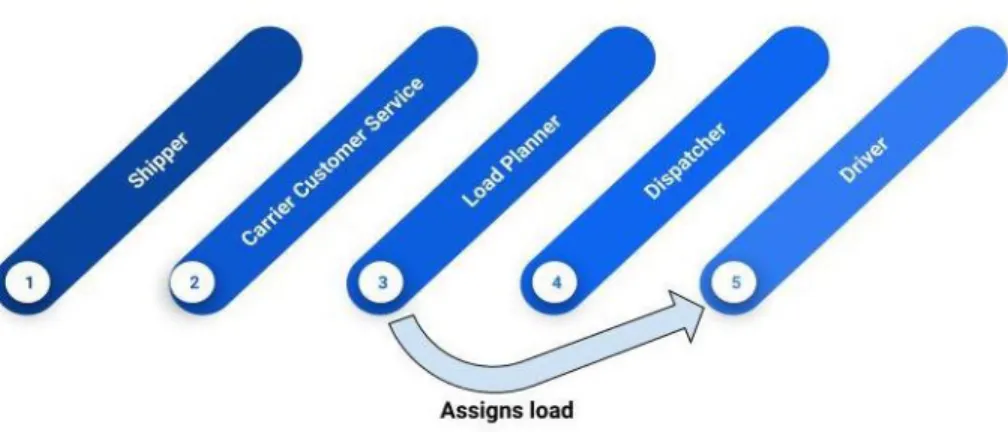
pre-established contract rates and lanes assigned. Carrier customer service representatives send requests to load planners, who assign loads to individual drivers or to a pair of drivers, known as a “team”. Between the load planner and the driver is the dispatcher, who sits physically at the carrier terminal location and is the driver’s point of contact for any questions or issues from assignment of a load to delivery at the receiver. At U.S. Xpress, one dispatcher is generally responsible for 60 drivers during the normal work week and up to 100 drivers during weekends and overnights. This is typical for other carriers of the same size. Load planners and dispatchers tend to operate with, at most, a three-day planning window. Figure 1 depicts this workflow.
22
Figure 1: Load Initiation and Assignment
Also important to this capstone is understanding the ways loads are picked up and dropped off. There are two methods: live load/unload and drop-and-hook. In a live load, a driver drives an empty truck to the shipper, and waits on-site while the trailer is loaded. Loading may be conducted by
employees of the shipper, or by a third party hired by the shipper - but in either case the driver does not usually assist. A live unload is the same but involves taking merchandise or equipment off the truck at the receiver’s location. Live loads/unloads should take no more than two hours. Per conversations with our sponsor company, we know this is the industry-recognized standard and often included in the contract between carriers and shippers. Drop-and-hook, by contrast, involves picking up or dropping off a completely loaded trailer at a shipper or receiver, respectively. This method is expected to take around 45 minutes - another industry standard - but can take much longer if trailers are blocked by other trailers during pick-up, or yards need to be reconfigured to make space for a drop-off. Regardless of the driver’s involvement, the time each load and unload takes counts toward the driver’s hours of service, so it is essential that they are conducted as efficiently as possible in order to maximize drivers’
23 3.1.2 Identification of Scope
To achieve results most useful to the sponsor company, we made decisions regarding capstone scope. First, we eliminated from consideration any corner cases: that is, any unique or rare situations occurring outside of normal operations. Second, we focused only on trips with contracted rates on established lanes, and we removed from the data any trips procured through the spot market. This decision eliminated some of the variability in scheduling and pricing that comes with the spot market; focusing on trends with key, contracted partners creates more relevant results and allows for more widely-applicable recommendations.
We also included only data from U.S. Xpress-employed drivers. While U.S. Xpress does utilize subcontractors on occasion, these represent a small subset of drivers. Subcontractors also have certain flexibilities that employees do not, such as the ability to turn down routes/loads; these factors would skew the dataset in a way that might render results less useful for U.S. Xpress.
For the purposes of this capstone, we are only considering loads driven by solo drivers. This focus allowed us to maintain 82% of the ELD dataset. Attempting to consider teams would have added a significant level of complexity, especially when considering utilization in terms of hours of service; team drivers have different rules and regulations around allotted working hours. By narrowing scope to solo drivers only, we were best able to test four hypotheses spanning several focus areas.
Finally, we do not include profit or revenue when considering driver utilization. While some companies in the industry look at total dollars earned per mile or week as a metric of productivity, we deemed this metric out of scope for this capstone and turn instead to hours of service. Through extensive conversation on the matter with the sponsor company, we believe hours of service to be the most useful way to look at utilization - and the one through which we can provide the most impactful recommendations.
24 3.1.3 Determination of Methodology
Kristen Eisenhardt describes a methodology approach that combines qualitative and quantitative data collection in order to best capture the dynamics in subjects of study (1989). Our approach is consistent with this framework. Through testing of our hypotheses, the datasets described below paint a picture of areas of opportunity by revealing consistent points of delay among drivers and along routes. To turn these findings into feasible recommendations, we sought a broader understanding of such situations through anecdotal information from drivers. Trends in the data show where problems occur, but insights from conversations are what ultimately will drive solutions.
The quantitative portion of our research included analyzing data from TMS and ELDs in U.S. Xpress trucks. The TMS data includes dates and times of stops along routes with associated location IDs (tied to shippers and receivers). This dataset also includes the corresponding driver ID number and the nature of the load/unload (either live or drop-and-hook). The latter is particularly important as it can vary greatly in duration. As previously mentioned, live loads/unloads are expected to take no more than two hours, and drop-and-hook loads/unloads are expected to take around 45 minutes. In practice, inefficiencies at shipping at receiving facilities or issues with driver appointments can often mean more time spent at their facilities no matter the method utilized.
The ELD data focuses primarily on the driver’s status, and includes location and hours of service available. We also utilized a driver dataset, which includes each U.S. Xpress driver’s unique ID, age, gender, and the number of months experience as a truck driver at the time they were hired by U.S. Xpress. The driver ID in this dataset was married with the ELD data to determine whether tenure, age, or gender have any effect on driving behaviors or trends.
The qualitative portion of our research came from telephone interviews. In preparation for these interviews, we completed the obligatory Institutional Review Board’s “Social & Behavioral Research Investigators” training. We spoke to drivers, operations managers, sales managers, and information
25
managers; it was important to us to create a roster of interviewees which included representatives from several areas of the trucking business. Through conversations with the sponsor company and our own research, we learned that employee relationships (particularly those between drivers and fleet
managers) are hugely impactful and for many reasons can impact a driver’s daily driving time; a diverse interviewee roster paints the clearest picture of these employee dynamics.
Our approach to interviews was guided by principles of respect and ethics learned in the training. As Fujii (2017) stipulates, it is important to speak the language of one’s interviewees in order to glean valuable information and reduce the risk of offending; thus, we prepared for interviews by learning the vocabulary of the trucking industry. We formulated a set of standardized questions to ask interviewees, found in Appendix B, but allowed for organic conversation insofar as it provided more helpful
information. While interviewing is not sufficient to provide a complete understanding of trucking dynamics, it complements quantitative findings and provides the basis for our recommendations. 3.1.4 Focus Areas: Nodes and Drivers
With the data outlined above, our focus and analysis took two directions: nodes and drivers. We began by examining individual nodes that make up driver’s routes. We explored whether the geographic location of a shipper or receiver node had an impact on whether a driver arrived late to a pick-up or drop-off appointment; further, we explored whether being late to an appointment meant more time spent at the node itself. Some of our early research revealed that load pick-up at shippers takes considerably longer than drop-off at receivers, due to the way ELDs operate in practice as well as the fact that pick-ups generally take more staging and preparation (Correll, 2019). In the case of drop-offs at receivers, there is the same issue of preparation - but of facility rather than load. While drop-and-hook is considered to be the faster drop-off method, we collected anecdotal information that drivers often have to wait for space to be cleared in a facility yard for a simple trailer drop.
26
We then examined utilization per individual driver. As previously addressed, we used the driver dataset in conjunction with the ELD and TMS sets to see how different driver attributes might impact hours driven. We expected to see older drivers and drivers with more months of experience achieving better utilization. Through various conversations, we learned that major players in the industry are advocating for the allowance of younger drivers, as they believe that a younger demographic may adapt better to the somewhat nomadic and isolated lifestyle of a trucker. However, we expected our results to show that older and more experienced drivers are, in fact, the “power players” in the trucking space. U.S. Xpress also thought it would be interesting to explore utilization by gender, and based on conversations with company leadership we expected our results would show that women experience less dwell than their male counterparts.
3.2 Data
3.2.1 Introduction
In this section, we will outline the steps taken to clean and process the datasets in order to better understand what driver utilization looks like. We examined six months of data, from June through November 2020; at U.S. Xpress, ELD data goes back a maximum of six months.
3.2.2 Dataset Descriptions 3.2.2.1 ELD Data
In the ELD datasets, entries, or “pings”, are recorded automatically by U.S Xpress’s ELD technology, Drivertech, every 15 minutes while the vehicle is in motion. Pings are also generated by certain events, to include change of driver status or when an order event occurs (for example, when a driver arrives at a shipper or receiver location). In the datasets, there are two different categories of statuses. The first category is trailer duty status, and there are four different statuses of note for this capstone: Allocated (AL), Available (AV), Dispatched Empty (DE), Dispatched (DP). AL means that a load is allocated to a trailer. Generally, this status comes from time at a shipper or consignee while the load is
27
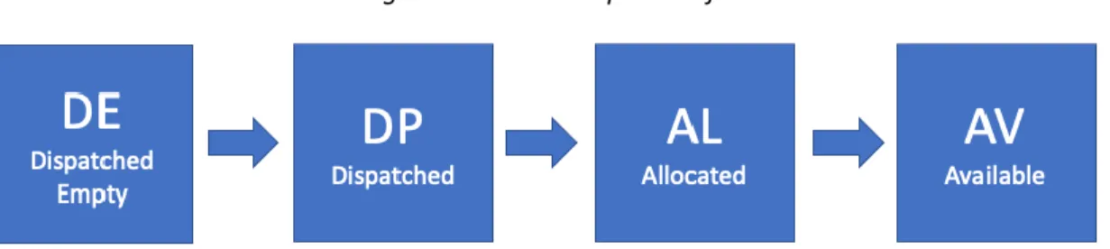
being loaded or unloaded. AV means that a trailer is ready for another load. DE suggests that a truck is driving but not carrying anything - these are known colloquially as “deadhead miles,” or miles for which the driver is not paid. DP means that the load is fully dispatched and the truck is on the way to its location - this represents loaded driving miles. The general sequence of these codes is depicted in Figure 2.
Figure 2: Normal Sequence of Statuses
The second category of statuses is driver hours of service status. There are four statuses of note in this category: On Duty, Off Duty, Sleeper Berth, and Driving. The former three statuses are considered non-driving time, and “On Duty” will be of particular importance when considering dwell, as it is the key indicator of status dwell.
In addition to these two status categories, the ELD dataset includes unique driver ID, tractor number, latitude and longitude at the time of the ping, the amount of time drivers have before their next required reset or restart.
3.2.2.2 Driver Data
This dataset includes basic information about each one of U.S. Xpress’s drivers. It includes Driver ID, age (as of June 1, 2020), gender, hire data, termination date (if applicable), and months of experience as a truck driver at the time of hire. It also includes each driver’s company, which is either 1 (employed by U.S. Xpress) or 63 (contractor/agent not considered a U.S. Xpress employee).
3.2.2.3 TMS Data
The TMS dataset includes data regarding orders, stops at terminals, shipper nodes, and receiver nodes, and whether or not loads at these nodes were live or drop-and-hook. In the dataset, there are
28
two methods by which arrival and departure time at nodes were captured: driver-recorded or
automatically captured by entry/exit gates at the nodes. We selected the driver-recorded as our method for analysis, because these columns had fewer null rows than the gate-recorded columns.
3.2.3 Data Cleaning
3.2.3.1 Driver Data
As we started cleaning the data, the first and simplest step was to create a more focused list of drivers. Using the driver dataset, we first filtered out any drivers with 63 in the company column; according to our U.S. Xpress sponsors, these drivers are not under normal dispatch and should not be considered in our analysis. Next, we removed any drivers who had been terminated. Finally, we removed any drivers hired after June 1, 2020. This resulted in a set of drivers who had been employed during the entire duration of our analysis period, and reduced the total number of drivers from 4,947 to 1,673.
3.2.3.2 ELD Data
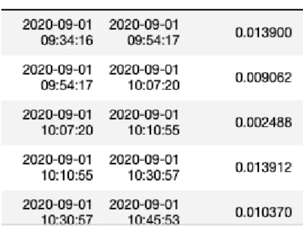
Our next step was to clean the ELD datasets. First, we merged the ELD dataset with the cleaned driver dataset on Driver ID, so that only the appropriately filtered drivers were reflected. Next, we wanted to understand how much time a given driver spent in each status (among both status categories, trailer and driver HOS) per week. To do this, we had to capture the time between each ping (in the datasets, ping logs are reflected in a column titled PositionDttm). After sorting the data by driver ID and by ping date time, we created two columns, Status_End and Time_In_Status. Status_End simply took the data from the PositionDttm column and shifted it up one, so that the start of one ping became the end of the previous ping. Time_In_Status took the difference between the two. Table 2 is an excerpt from the September ELD dataset, and provides an example of these column additions and associated calculations. Because some of these pings span across multiple days, the unit of measure for
29
Table 2: Depiction of Status_End and Time_In_Status Columns
With this clean dataset, even before any testing, we could create pivot tables and graphs depicting the time each driver spent per week in each status type. This helped us to get an initial sense of trends.
3.2.3.3 TMS Data
Our sponsor company asked us to remove terminals from this dataset, as they were more interested in exploring dwell at shipper and receiver nodes. We dropped from the dataset any rows with a stop type of ‘TT’, as this denotes a terminal stop. As previously mentioned, we chose to utilize driver-reported arrival and departure times at nodes. We removed from the dataset any rows in which these fields were null, which dropped less than 2% of the total dataset. The next step was to figure out exactly how to capture dwell in this dataset. We decided to look at the time spent at each node, considering the type of load (live or drop-and-hook), and compare that time spent to the industry norms for load type (2 hours for live, 45 minutes for drop-and-hook). If the time spent at a node exceeded these target times, the delta between the two would reflect nodal dwell. To do this, we first created a column called Time_At_Node, and populated this column with driver-reported departure time minus driver-reported arrival time. As was the case with the ELD datasets, some of these node visits spanned over a day, so the unit of measure for Time_At_Node is days.
30
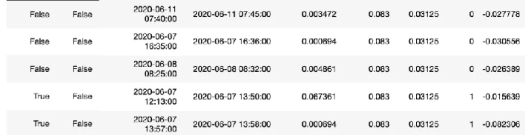
Next, we needed to create columns by which to compare this Time_At_Node column. We created two columns to represent the industry norms for both types of loads, calculated in days for consistency. We populated the live load target column, Target_Live, with .083 (2 hours, in days) and the drop-and-hook target column, Target_DH, with .03125 (45 minutes, in days).
Is_Live was coded to populate 1 if either the live load or live unload columns were true, and a 0 if both were false. This allowed us to easily segment the data into live and drop-and-hook loads/unloads for analysis.
Dwell was coded to subtract Target_Live from Time_At_Node where Is_Live=1, and to subtract Target_DH from Time_At_Node where Is_Live=0. This was necessary to ensure that the time spent at the node was being compared to the appropriate target metric. Table 3 depicts the framework of this approach.
Table 3: Depiction of TMS Dataset Manipulation
To prepare to test for driver lateness to appointments, we created a column called Is_Late, which compared driver-reported stop time with the end of the corresponding appointment window. If the stop time was later, Is_Late populated with 1. We then created a column called Amount_Late which took the difference between driver-reported stop time and the end of the appointment window time, to reflect how late the driver was to his or her appointment at the node.
31
The results of our four hypotheses are presented below. Our hypotheses covered a wide variety of factors potentially impacting driver utilization and dwell; our results show that some were more relevant than others. While we believe that each result provides interesting takeaways, most actionable insights come from the results of hypotheses II and IV.
4.1 Hypothesis I
Hypothesis I: Nodal dwell is consistently highest in nodes closest to American Transportation Research Institute (ATRI) bottlenecks. Proximity to bottlenecks increases lateness to appointments which in turn
increases nodal dwell. We expect that this is true over all months observed.
This hypothesis was born out of the idea that if drivers passed through bottlenecks, they were more likely to be late to appointments - and if they were late to an appointment, they were more likely to have more dwell at the node. To test this hypothesis, we used a haversine formula in Python to calculate the distance between each shipper and receiver node, and seven of the top ten ATRI
bottleneck locations which are in the same geographies as U.S. Xpress operates. The haversine formula takes the latitude and longitude of two locations and calculates the distance between them, considering the curvature of the earth. This meant that our TMS data frame now included columns for each of the seven bottleneck latitudes and longitudes, and the distance from each row’s node location to each of these bottlenecks. To test the hypothesis, we looked specifically into any bottlenecks that were within 20 miles of a node.
Surprisingly, our results suggest that proximity to a bottleneck does not contribute to lateness to an appointment. Notably, there were some instances in the dataset where the Amount_Late calculation came out to be quite large. According to our sponsor company, this may have been the result of an appointment time being formally changed and that change not being properly logged/reflected in the data - or some other unique, corner case situation. For this reason, they asked us to filter the data frame to only instances where Amount_Late was under 36 hours, or 1.5 days. Table 4 summarizes lateness
32
across the dataset, and lateness across only nodes within 20 miles of one of the seven bottlenecks. While drivers going to nodes within 20 miles of a bottleneck were late to appointments 3% more of the time, the amount by which they were late was actually smaller.
Table 4: Lateness Results
Total Instances Instances Late Percentage Late Average amount Late, when late
Across Dataset 368803 79009 21% 7.23 hours
Nodes w/in 20 miles of bottleneck
21447 5119 24% 5.61 hours
33
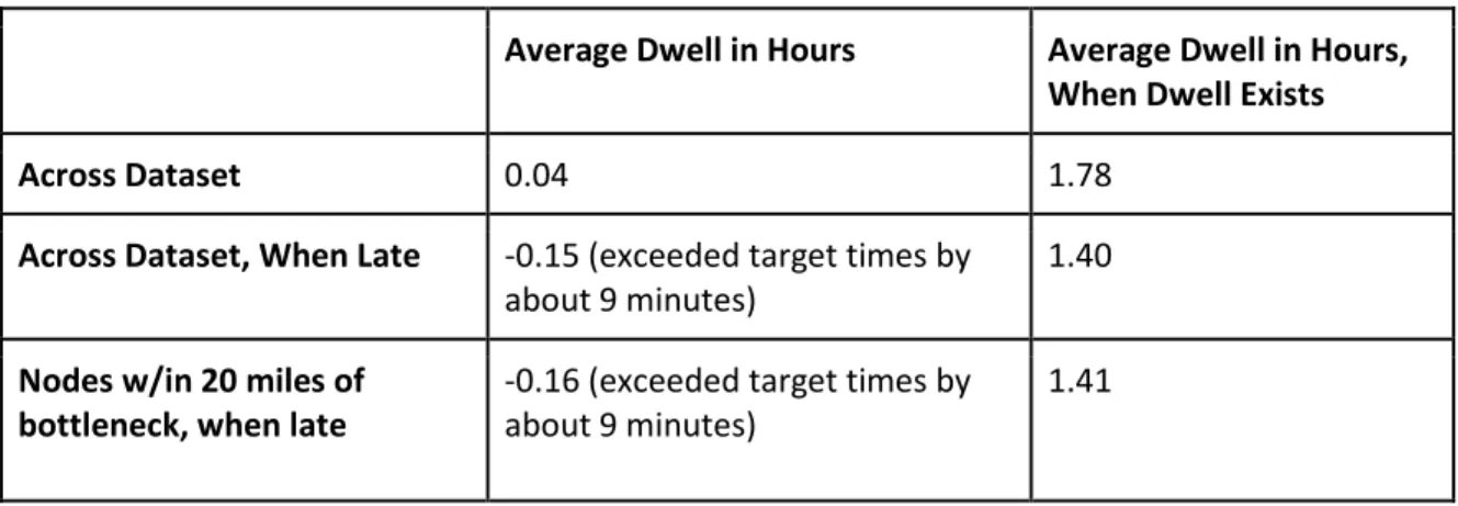
Perhaps even more surprisingly, our results suggest that arriving late to an appointment - whether close to a bottleneck or not - does not impact nodal dwell. As discussed in Chapter 3, nodal dwell is defined as time spent over the industry-recognized thresholds for live or drop-and-hook
loads/unloads. It is calculated by taking the time spent at the node, minus the threshold time - a positive result would represent the time over threshold, and a negative result would represent the amount of time under a threshold (colloquially, the amount of time by which time at a node “beat” the target). Notably, there were some instances in the dataset when the nodal dwell calculation was quite large. This may be the result of a driver taking his overnight break at a node, or some other unique, corner case situation. For this portion of the analysis, our sponsor company asked us to filter the data to only instances where nodal dwell was less than 10 hours, to eliminate these cases. In Table 5, the rightmost two columns represent instances only when nodal dwell was present - that is, instances in which the dwell column was greater than 0.
Table 5: Dwell and Lateness Results
Average Dwell in Hours Average Dwell in Hours, When Dwell Exists
Across Dataset 0.04 1.78
Across Dataset, When Late -0.15 (exceeded target times by about 9 minutes)
1.40
Nodes w/in 20 miles of bottleneck, when late
-0.16 (exceeded target times by about 9 minutes)
34
Figure 4: Average Dwell at Node by Distance to Closest Bottleneck, When Dwell Exists
We performed a regression analysis to test this hypothesis by setting a binary variable of 1 for nodes within 20 miles of a bottleneck and comparing it to the resulting dwell and total time spent at the node. Our findings are summarized in Table 6: Hypothesis I Regression Results for Dwell and Table 7:
Hypothesis I Regression Results for Time at Node.
Table 6: Hypothesis I Regression Results for Dwell
R Square 0.06
Observations 451559 Coefficient 0.09 Standard Error 0.01
35
Table 7: Hypothesis I Regression Results for Time at Node
R Square 0.02
Observations 451559 Coefficient 0.09 Standard Error 0.01
P-value < 0.01
Based on these regression outputs, we reject the null hypothesis and determine that proximity of a node to an ATRI-identified bottleneck is not a significant determinant of driver dwell.
4.2 Hypothesis II
The type of load or unload and time of day a driver arrives impact nodal dwell.
IIa. Nodal dwell is significantly higher at nodes that utilize live loads and unloads than those that use drop-and-hook.
IIb. Dwell is lowest at peak node activity times.
Through conversations with those in the trucking industry and transportation researchers, it is evident that drop-and-hook loads/unloads are strongly preferred across the board. Perhaps since the industry-recognized threshold for a drop-and-hook is much shorter (45 minutes, as compared to 2 hours for live), and since drop-and-hook is designed to require less manpower at a shipper or receiver node, this method is presumed to be the more efficient one. We expected that this would prove true within U.S. Xpress operations. Before narrowing our focus to dwell, we found it helpful to consider total time at each node by load/unload type and hour. Figures 5 and 6 illustrate this view. Figure 6 is a histogram showing the amount of time at nodes in 30-minute (.5 hour) bins, for both types of load/unload.
36
Figure 5: Time at Node by Hour of Day
37
Generally, we observe that drop and hooks are faster than live loads and unloads and both kinds of loads are fastest during the day. With a broader view established, we considered nodal dwell. Table 8 represents nodal dwell for both types of load/unload, and the rightmost two columns represent only instances where dwell was present - that is, instances in which the dwell column was greater than 0.
Table 8: Dwell by Load/Unload Type
Average Dwell in Hours Average Dwell in Hours, When Dwell Exists Live Load/Unload -0.66 (shorter than target times
by about 40 minutes)
1.99
Drop-and-Hook Load/Unload 0.36 1.27
These results are interesting: on average, when conducting a live load/unload, U.S. Xpress drivers are actually averaging shorter than target time, while drop-and-hooks average about 22 minutes over target time. However, considering only instances where dwell was present, live loads did exhibit a greater amount of dwell as compared to drop-and-hook.
We looked further into how dwell was distributed by hour of day, for both live and drop-and-hook loads/unloads. Benjatanont and Tauntico (2020) and Buttgenbach and Zhang (2020), analyzing two different trucking firms, both found that time spent at nodes was lowest during peak node activity time (that is, when nodes had the highest volume of deliveries and pick-ups). For drop-and-hook
loads/unloads, our findings were consistent with the aforementioned. Specifically, Benjatanont and Tauntico presented evidence suggesting that time spent at nodes was lowest between 6am and 3pm; our results show dwell steadily decrease during these hours. Figure 7 depicts average dwell per hour for drop-and-hook and live loads and unloads; the x-axis represents hour of day on a 24-hour clock.
38
Figure 7: Nodal Dwell by Hour of Day
We performed a regression analysis to test this hypothesis by designating “on-peak” and “off-peak” times, defining “on-“off-peak” as between 7am and 5pm, which is based on our understanding of normal node hours. From there, we created three binary columns, “Drop and Hook during On-Peak”, “Drop and Hook during Off-Peak”, and “Live Load during Off-Peak”. We performed a regression analysis on these variables against resulting dwell and total time spent at the node. The results, and a summary of time at node for both types of load/unload and on-peak/off-peak are shown in Tables 9, 10. and 11.
39
Table 9: Hypothesis II Regression Results for Dwell
R Square 0.06
Observations 451559
DH_Off_Peak Live_Off_Peak DH_On_Peak
Coefficients 1.05 0.51 1.01
Standard Error 0.01 0.01 0.01
P-value < 0.01 < 0.01 < 0.01
Table 10: Hypothesis II Regression Results for Time at Node
R Square 0.02
Observations 451559
DH_Off_Peak Live_Off_Peak DH_On_Peak
Coefficients -0.29 0.51 -0.24
Standard Error 0.01 0.01 0.01
P-value < 0.01 < 0.01 < 0.01
Table 11: Average Time at Node, Summarized
Based on these results, we do not reject the null hypothesis and contend that nodal dwell is lowest during peak hours of operation, with live loads and unloads seeing the strongest effect of this timing.
40 4.3 Hypothesis III
Driver demographics have an impact on driver dwell (time spent in On Duty Status).
III a. Drivers under the mean company driver age of 43 experience more dwell than their older counterparts due to lack of time management experience.
III b. Drivers with more months of experience experience less dwell. III c. Female drivers experience less dwell than their male counterparts.
Through our research, and through conversations with drivers and others in the industry, we learned that experience goes a long way in the trucking world. Particularly at nodes, more experienced drivers are more likely to have identified best practices - best points of contact, for example - that help them get in and out faster. In addition, we cannot ignore the reality that older drivers may simply be better at managing their time clocks - since experienced drivers would have started logging their hours of service manually and then migrated to ELDs, they may have brought with them some learned practices on how to optimize their time.
To test this hypothesis, we first needed to get a sense of the distribution of driver ages and genders. The data described below was cleaned as outlined in section 4.3.1. Figures 8 reflects these distributions.
41
We utilized six months of ELD data to test this hypothesis. We define dwell a bit differently in this dataset, as compared to the TMS one; here, dwell is considered time spent in On Duty status and referred to as status dwell. Conversations with our capstone sponsors confirmed the fact that this is the best way to explore dwell along a driver’s trip; time in On Duty status does count against their 14-hour allotted workday, but it is time not spent driving. To test this hypothesis, we grouped by Driver ID Number and aggregated time in On Duty status, to see how much time was spent in this status per week. We also included driver age, experience, and gender.
For hypothesis III-a, we performed a regression analysis expecting to see a clear negative correlation between age and time in On Duty status. Figure 9 reflects the average time spent in On Duty status per week in hours, against driver age.
42
For hypothesis III-b, we expected to see a clear negative correlation between driver months of experience and time in On Duty status. Figure 10 reflects the average time spent in On Duty status per week, against driver experience.
Figure 10: Average Time in On Duty Status per Week vs. Driver Experience
For hypothesis III-c, we expected to see that female drivers experience less status dwell than their male counterparts. Figure 11 reflects the average time spent in On Duty status per week by gender.
43
Figure 11: Average Time in On Duty Status per Week vs. Gender
These box-plots provided very similar results and showed that the mean time in “On Duty” status for female drivers was 5.00 hours for women versus 5.12 hours for men each week. This is not a statistically significant difference, which disproves this hypothesis and we can conclude that men and women drivers experience the same dwell. We performed a regression analysis on all of these variables which returned the results shown in Table 11.
Table 11: Hypothesis III Regression Results for Dwell R Square 0.01
Observations 34612
Gender_is_Female Older_Than_43 Total_Experience
Coefficients 0.77 -1.14 0.01
Standard Error 0.23 0.15 0.01
44
Based on these results, we reject the null hypothesis: drivers’ gender, age, and total experience do not play a significant factor in determining the status dwell they experience.
4.4 Hypothesis IV
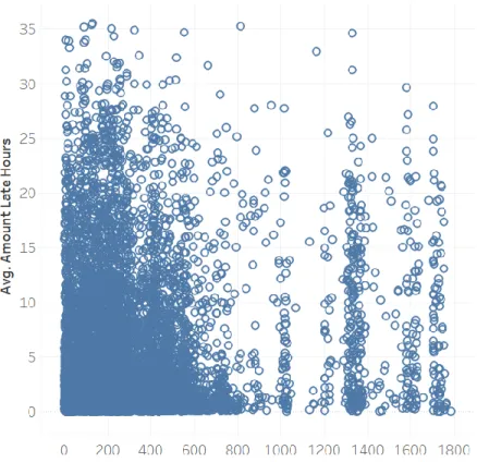
Drivers who repeatedly visit the same nodes experience less nodal dwell as their number of visits increases.
To test this hypothesis, we merged ELD and TMS data to match Driver IDs with order numbers and specific trips. We reverted to the same definition of dwell as in Hypotheses I and II, nodal dwell, as our aim was to determine dwell for each driver at the nodes themselves. To create Figure 12, we counted the distinct number of orders between each driver and node and used that as a proxy for the number of visits. Then we compared that number to the average dwell the driver experienced every time he or she visited the node.
Figure 12: Average Dwell per Node Visit by Count of Visits of Driver to Node
We also considered total time at node for live and drop and hook loads and unloads, shown in Figures 13 and 14. Their results mirror the nodal dwell results in Figure 12.
45
Figure 15: Average Time at Node by Count of Visits of Driver to Node, Live
Figure 16: Average Time at Node by Count of Visits of Driver to Node, Drop and Hook
In order to evaluate this relationship, we performed a logistic regression with total time at node versus number of visits by a driver to the node. Results of this analysis are shown in Table 12.