The effect of flight simulator motion on modelled vestibular response

THE EFFECT OF FLIGHT SIMULATOR MOTION ON MODELLED VESTIBULAR RESPONSE

by

Kathleen M. Misovec

B.S., Massachusetts Institute of Technology, 1984 Submitted in Partial Fulfillment

of the Requirements for the Degree of

Master of Science in Aeronautics and Astronautics at the

Massachusetts Institute of Technology September, 1986

()Massachusetts Institute of 1986

Signature of Author

Technology

Department of Aeronautics and Astronautics September, 1986

Certified by

Professor Steven R. Bussolari Thesis Supervisor Certified by

Professor Harold Y. Wachman Chairman Departmental Graduate Committee Department of Aeronautics and Astronautics

mITLibraries

Document Services

DISCLAIMER OF QUALITY

Due to the condition of the original material, there are unavoidable

flaws in this reproduction, We have made every effort possible to

provide you with the best copy available. If you are dissatisfied with

this product and find it unusable, please contact Document Services as

soon as possible.

Thank you.

Some pages in the original document contain pictures,

graphics, or text that is illegible.

THE EFFECT OF FLIGHT SIMULATOR MOTION ON MODELLED VESTIBULAR RESPONSE by

Kathleen M. Misovec

Submitted to the Department of Aeronautics and Astronautics on August 30, 1986 in partial fulfillment of the requirements for the Degree of Master of

Science in Aeronautics and Astronautics ABSTRACT

A study of the effect of flight simulator motion on modelled vestibular response was conducted. Experiments were performed on a Boeing 727 flight simulator which used a synergistic motion base. Three different motion conditions were compared in the experiments. One condition consisted only of high frequency, low amplitude special effects such as turbulance and landing gear extension. The second condition, jostle motion, consisted of motion capability in the lateral and vertical degrees of freedom as well as special effects. The third condition, full motion, was the six degree of freedom capability normally used on the flight simulator.

Three flight scenarios, designed to require significant amounts of pilot control activity, were flown by eighteen subjects. The subjects were divided into three groups of six, each group performing one scenario. The first scenario consisted of an engine flame out on take off. The second, an airwork scenario, consisted of steep turns, approach to stall maneuvers, and standard rate turns with yaw damper failure. The third scenario was an ILS approach and landing in wind shear.

The two primary types of measurements that were analyzed were acceleration errors and vestibular errors. Acceleration error is defined to be the

difference between the accelerations of the aircraft and the simulator.

Vestibular error is defined to be the difference between the pilot's modelled vestibular responses in the aircraft and the simulator. Two other sets of measurements, pilot opinion and pilot performance, were also compared for

the three motion conditions of the experiment.

In general, no significant differences were found between the motion conditions for any of the measurements. However, for the vestibular error measurments, the rotational vestibular errors were usually below established

thresholds of perception while many of the translational errors were above the thresholds of perception.

Thesis supervisor: Steven R. Bussolari, PhD

ACKNOWLEDGEMENTS

I would like to thank my father, Dr. Andrew Misovec. His ideas and our conversations about engineering have always been extremely valuable to my education. His constant encouragement and insights are greatly appreciated.

Professor Steven Bussolari provided the basic idea for the experiments and contributed to thcir implementation and analysis. I would like to thank Dr. Alfred Lee for the analysis of performance data and Ted Demosthenes for his generous help with running the experiments. Thanks are due to Dr. Charles Oman for consultations about the vestibular models and to Dr. Alan Natapoff for consultations about the statistical analysis of the data.

Conversations with Dr. Mohammed Massoumnia have been extremely valuable to my general education and are greatly appreciated. I would also like to thank Ed Kneller, Mark Shelhamer and R. Bryan Sullivan for their helpful thoughts on the technical aspects of the analysis of these experiments.

Thanks also to Dan Merfeld for his ideas. The generous amounts of advice and help from Sherry Modestino and Ed Kneller in writing and preparing this

thesis are gratefully acknowledged.

I am grateful to Margaret Misovec, Mary Misovec, Paul Misovec, Andrew C. Misovec, Michael Misovec, James Smith, Patricia Tellier and Rene Tellier for their support and encouragement. Thanks also to Kevin Ackley, Marilyn Cieuzo, Suzanne Cox, Wayne Greene, Justin Marble and Jennifer Wiseman.

TABLE OF CONTENTS

CHAPTER 1: INTRODUCTION . . . . . . . . . . . . . . . . . . . . . . . . . 5

1.1 Types of Motion Systems . . . . 7

1.2 Types of Washout Systems . . . . . . . . . . . . . . . . . . . 13

1.3 Problems with the Optimal Control Washout Design - What Should Be Optimized? . . . . . . . . . . . . . . . . . . . . . . . . 17

1.4 Problems Associated with Quantifying Simulator Realism . .... 17

1.5 This Research - More Basic Questions . . . . . . . . . . . . . 21

1.6 Thesis Outline . . . . . . . . . . . . . . . . . . . . . . 23

CHAPTER 2: FORMULATION OF THE VESTIBULAR ERROR AS A MOTION FIDELITY MEASURE . . . . . . . . . . . . . . . . . . . . . . . . . . 24

2.1 Introduction .. .. '. . . . . . . . .. .. . 24

2.2 Semicircular Canals . . . . . *.. .. .. ... . . . .. . . 24

2.2.1 Physical Description of the Semicircular canals . . . 24

2.2.2 Mathematical Model of the semicircular canals . . . . . 25

2.3 Otoliths . . . . . . . . . . . . . . . . . . . . . . . . . . . 33

2.3.1 Physical Description of Otoliths . . . . . . . . . . . . 33

2.3.2 Mathematical Models of the Otoliths . . . . . . . . . . 33

2.4 Vestibular Error Measurements . . . . . . . . . . . . . . . . 35

CHAPTER 3: EXPERIMENTAL DESIGN AND ANALYSIS MEASUREMENTS . . . . . . . 40

3.1 Brief Introduction . . . . . . . . . . . . . . . . . . . . 40 3.2. Experiment Description . . . . . . . . . . . . . . . . . . . 40 3.2.1 Simulator . . . . . . . . . . . . . . . . . . . . . . 40 3.2.2 Motion Conditions . . . . . . . . . . . . . . . . . . 40 3.2.3 Flight Scenarios . . . . . . . . . . . . . . . . . . . 42 3.2.3.1 Familiarization Scenario . . . . . . . . . . . 43

3.2.3.2 Engine flame-out on takeoff . . . . . . . . . . 43

3.2.3.3 Airwork Scenario . . . . . . . . . . . . . . . 44

3.2.3.4 ILS Approach and Landing Scenario . . . . . . . 44

3.2.4 Subjects . . . . . . . . . . . . . . . . . . . . . . . 46

3.2.5 Order Effects . . . . . . . . . . . . . . . . . . . . 47

3.3 Analysis Measurements. . . . . . . . . . . . . . . . . . . . . 47

3.3.1 Opinion Measurements. . . . . . . . . . . . . . . . . . 47

3.3.2 Acceleration Error Measurements . . . . . . . . . . . . 51

3.3.3 Vestibular Error Measurements . . . . . . . . . . . . 52

3.3.4 Pilot Performance Measurements. . . . . . . . . . . . . 53

3.3.4.1 Engine Flame-out Scenario . . . . . . . . . . . . 53

3.3.4.2 Airwork Scenario. . . . . . . . . . . . . . . . . 53

3.3.4.3 ILS Approach and Landing Scenario . . . . . . . . 54

3.4 Data Collection . . . . . . . . . . . . . . . . . . . . . . . 54

3.4.1 Variables . . . . . . . . . . . . . . . . . . . . . . . 54

3.4.2 Trials . . . . . . . . . . . . *. * . . .. . . . . . . . 57

3.4.3 Pertinent Degrees of Freedom for Each Scenario . . . . 57

3.4.4 Data Windows . . . . . . . . . . . . . . . . . . . . . 58

3.4.5 Data Collection Problems . . . . . . . . . . . . . . . 59

3.4.5.1 Possible Aliasing of Rotational Data . . . . . . 59

3.4.5.2 Lateral Axis Data . . . . . . . . . . . . . . . . 60

3.4.5.3 Longitundinal Axis Acceleration Data. . . . . . . 60

CHAPTER 4: PILOT OPINION RESULTS AND DISCUSSION . . . . . . . . . . . . 62

4.1 Introduction . . . . . . . . . . . . . . . . . . . . . . . . 62

4.2 Presentation of Opinion Results . . . . . . . . . . . . . . . 62

4.3 Discussion of Pilot Opinion Results. . . . . . . . . . . . . . 64

CHAPTER 5: ACCELERATION ERROR RESULTS AND DISCUSSION . . . . . . . . . 70

5.1 Introduction . . . . . . . . . . . . . . . . . . . . . . . . 70

5.2 Engine Flame-Out Acceleration Error Results . . . . . . . . 71

5.3 Steep Turu Acceleration Error Results . . . . . . . . . . . . 72

5.4 Stall Acceleration Error Results . . . . . . . . . . . . . . 75

5.5 Rate Turns with Yaw Damper Failure Acceleration Error Results. 78 5.6 ILS Approach and Landing Scenario Results . . . . . . . . . 80

5.6.1 Approach Segment: 500' - 200' . . . . . . . . . . . . 80

5.6.2 Landing Segment: Last 20 to 25 s Before Touchdown . 83 5.7 Discussion. ... ,. ...'.. ... ... 86

5.7.1 Discussion of Analysis Method. . . . . . . . . . . . . . 86

5.7.2 Discussion of Results. . . . . . . . . . . . . . . . . . 88

CHAPTER 6: VESTIBULAR ERROR RESULTS AND DISCUSSION . . . . . . . . . 90

6.1 Engine Flame-Out Vestibular Error Results . . . . . . . . . . 91

6.2 Steep Turn Vestibular Error Results . . . . . . . . . . . . . 92

6.3 Stall Vestibular Error Results . . . . . . . . . . . . . . . . 95

6.4 Rate Turns with Yaw Damper Failure Vestibular Error Results . 98 6.5 ILS Approach and Landing Vestibular Error Results. . .... 101

6.5.1 Approach Segment: 500' - 200' . . . . . . . . . . . . 101

6.5.2 Landing Segment: Last 20-25 sec before touchdown . . 105

6.6 Discussion of Vestibular Error Results . . . . . . . . . . . 109

CHAPTER 7: PILOT PERFORMANCE RESULTS . . . . . . . . . . . . . . . . . 111

7.1 Engine Flame-Out Performance Results . . . . . . . . . . . . 111

7.2 Airwork Scenario Performance . . . . . . . . . . . . . . . . 112

7.2.1 Approach-to-Stall . . . . . . . . . . . . . . . . . . . 112

7.2.2 Rate Turns with Yaw Damper Failure . . . . . . . . . . 112

7.3 ILS Approach and Landing Scenario . . . . . . . . . . . . . 112

7.4 Discussion of Performance Results. . . . . . . . . . . . . . . 113

CHAPTER 8: PROBLEMS DUE TO ALIASED ROTATIONAL VESTIBULAR RESPONSES . . 117

8.1 Introduction . . . . . . . . . . . . . . . . . . . . . . . . 117

8.2 Aliasing General Information . . . . . . . . . . . . . . . . 117

8.3 The Effect of Undersampling on the Results of This Study . . 119

8.4 Rotational Vestibular Error Results . . . . . . . . . . . . . 119

CHAPTER 9: CONCLUSIONS AND RECOMMENDATIONS . . . . . . . . . . . . . . 131

9.1 Conclusions . . . . . . . . . . . . . . . . . . . . . . . . . 131

9.2 Recommendations . . . . . . . . . . . . . . . . . . . . . . 132

CHAPTER 1: INTRODUCTION

In addition to being useful as both subjects and tools of scientific research, flight simulators provide training to aircraft pilots, and are also used for pilot certification. Pilot training and certification encompasses a broad range of flight manuevers from standard procedures such as cruise to more complicated and frequently dangerous manuevers such as an engine failure on takeoff. Performance of such manuevers in a simulator instead of an actual aircraft is valuable for two reasons. One is because if a pilot makes a mistake in an actual aircraft, collision is possible. The

other is that although simulators may have a higher initial cost than the actual flight vehicle, the operational costs of simulators are usually less than those of an actual flight vehicle. This

makes pilot training and certification less expensive in a simulator in an actual aircraft.

It is vitally important that the simulation is realistic enough so that pilot training received in simulated emergency manuevers

is adequate enough to apply to similar situations that may arise in an actual aircraft. Currently it is not known how realistic the simulator must be to achieve adequate "transfer-of-training" from simulator to aircraft. So the effort has been to make the simulation as realistic as possible. There are three general types of realism. Engineering realism may be parameterized by dynamic characteristics such as accelerations and forces. Psychological realism could be achieved by such factors as an actual instrument panel, or realistic air traffic control simulation and could be measured by pilot opinion about the fidelity of the simulation.

Physiological fidelity pertains to the accurate representation of sensory signals sent to and processed by the central nervous system.

A natural tradeoff arises between the fidelity of the simula-tion and the cost associated with the complexity of the system. The lower fidelity flight training systems might be a cardboard representation of the instrument panel or relatively simple program that runs on a microcomputer. Both realism and cost are increased as real instruments and an actual cockpit setting, which provide primarily psychological fidelity, are added to the system. Physio-logical as well as psychoPhysio-logical fidelity can be increased, at

high financial cost, by including a visual system in the simulation. A motion system may increase engineering, psychological and physio-logical realism to the simulation. In recent years, technophysio-logical

improvements in motion systems have been mainly software-oriented so that their cost, which is high primarly due to dynamic require-ments of obtaining accelerations, remains relatively high.

Most of the more advanced simulators today have highly complex, expensive motion systems. Many motion systems have been installed and methods of controlling the motion base have been widely

researched because of an implicit assumption that motion capability in a simulator is critical for realism and therefore necessary for adequate transfer-of-training from simulator to aircraft. The goal of this thesis is to scientifically examine this assumption by comparing the effects of different levels of motion capability

on various parameters of engineering, psychological and physio-logical realism.

1.1 Types of Motion Systems

There are six possible independent directions or degrees of freedom in which motion capability is possible in all physical unconstrained systems. As shown in Figure 1.1, there are the

three translational degrees of freedom and three rotational degrees of freedom. In this thesis, the translational degrees of freedom will be referred to as "surge" for longitudinal motion; "sway" for

lateral motion, and "heave" for vertical motion. While the rota-tional degrees of freedom will be referred to as "pitch", "yaw", and "roll"

IVarer&I

Figure 1.1: The six possible degrees of freedom of motion.

There are a variety of different mechanical ways to produce simulator motion currently in use. In cascaded systems, such as that shown in Figure 1.2, each degree of freedom is separately and independently controlled by a cascade of six motion elements. Translational degrees of freedom are achieved by allowing a cab to

move on a cascade of linear tracks. This motion is characterized by the position, velocity and acceleration of the cab along the tracks. The length of the track limits translational motion capabi-lity. Rotational directional capability is acheieved by suspending the cab in a motor-driven gimbal. Three nested gimbals are needed to obtain complete rotational capability about any axis. Rotational motion is limited by the maximum angular positions, angular velo-cities, and angular accelerations that the system can undergo.

In other systems, known as synergistic simulators, the actu-ators work together to achieve motion in a single degree of freedom (see Figure 1.3). This can be achieved by having a cab supported by a platform which is supported by six legs attached to the ground.

The legs are controlled by hydraulic pistons and limitations are due to the maximum length of the legs and the their maximum rates of change. The maximum force that the legs can generate is another motion capability limiting factor. The primary advantage of this

"hexapod" system over the cascaded system is that the hardware is simpler.

Some systems, such as the Vertical Motion Simulator (VMS) located at NASA Ames, have a motion base system that is a combina-tion of the cascade and the hexapod system. In the VMS, as shown in Figure 1.4, linear tracks provide the translational motion capab-ilitities, while a hexapod system provides the rotational capabi-lities. Although there are only two tracks in this system, the cab can rotate about a vertical axis to allow the horizontal track

to be used for both longitudinal and lateral motion (Sullivan, 1985).

Another type of system is exemplified by the Large Amplitude Multi-Mode Aerospace Research Simulator ("LAMARS") located at Wright-Patterson Air Force Base. In this system, a 10 meter beam

suspends a large sphere which supports the simulator cab. The beam is capable of lateral and vertical motions. The cab is gim-balled so that it can move in all three rotational degrees of

freedom.

Centrifuge motion systems are gimballed cabs that are suspended at the end of a large rotating arm (see Figure 1.5). The design of a controller for these motion systems is challenging because the pilot is in a rotating environment. Unlike the above systems which are only capable of half of a g acceleration levels, centrifuge motion systems can achieve translational accelerations of up to 40g (Ish-Shalom, 1982). The capability of large sustained acceler-ation is extremely useful in training military pilots to avoid blacking out, which happens ocassionally when they are flying high performance fighter aircraft. The high g-levels can draw the blood from their heads and cause them to lose consciousness. One of the highest fidelity flight simulators currently in existence are vari-able stability airplanes that are used as flying simulators. These planes are designed so that their natural frequencies can be varied to simulate different types of aircraft.

CDC199I MSPILAT AI=ZaS P.ATFORM PITCH AXIS YISUAL O3KAT c-zAagpg curxia t"ie AXIST Faci2 A, 977T

CA4043 (WCA -liCA4.

Figure 1.2 Example of Cascaded Motion Base System (Sinacori, 1977)

Figure 1.3: Example of Synergistic Motion Base System (Unscaled Drawing)

Figure 1.4 Vertical Motion Simulator (VMS) (Sullivan,1985)

IVon-Gierke

Figure 1.5: Artist's Conception of ,cntri'uge Motion Base System (7on-Gierke 19(a

1.2 Types of Washout Systems

Designing a simulator motion drive logic system is a challeng-ing control problem. The basic task is to compute simulator motion base commands on the basis of computed airplane motions without exceeding the limitations of the motion system, while retaining as much realism as possible (Figure 1.6) (Ish-Shalom, 1982). The term "washout system" is given to the simulator controller because basically the system undergoes an initial acceleration in some direction that must be slowly faded or "washed" out so that the simulator will not reach the limits of its excursion capabilities. Afterwards, the simulator, which has changed position as a result

of the acceleration, is slowly allowed to return to a more central position so that it can have enough room for travel in the next portion of the flight. Ideally the system should be designed so

that the whole procedure is as realistic as possible to the pilot. For example when the simulator accelerations are being washed out and when the simulator returns to a central position, it should do so in such a way that the motions involved are below the threshold of perception in the pilot.

There are a variety of washout systems that are currently in use in industry today. Examples of the simpler types of washout systems in use are systems that employ some sort of acceleration-matching strategy. For example, the simulator acceleration could be the actual aircraft acceleration multiplied by a constant gain. The "clipped magnitude" concept, another example of this type of washout system, matches the accelerations as long as they don't exceed a certain limit dictated by the capabilities of the

simulator. One of the disadvantages of these systems is that they are not self-centering. Other disadvantages include the facts that the proportional drive needlessly limits low displacement high frequency accelerations; while the clipped magnitude drive unnec-essarily limits high frequency high amplitude accelerations that are still within the excursion limits of the simulator.

More complicated washout systems in use today represent the simulator motion drive logic problem in the frequency domain and thus are able to employ techniques which take advantage of what has happened earlier in the simulation. By extrapolating knowledge

about rates of change, these types of systems are also able to make and act upon predictions about what will happen next in a

simulated flight. In other words these simulators have memory. An example of this type of system is the linear crossfeed washout, which uses second order high-pass filters with cross coupling between translational and rotational degress of freedom. By

tilt-ing the simulator below the perception level of the pilot, this type of system is also able to take advantage of the component of gravity to obtain longitudinal and lateral accelerations and thus minimize undesired accelerations in these directions (see Figure

1.7). Another type of washout system is the linear quadratic opti-mal control system. In this method, after certain assumptions are made, a quadratic cost functional, which represents the engineering

tradeoffs being made, is minimized. (Sivan et al., 1982, Sturgeon, 1981, Ish-Shalom, 1982) Other examples include a non-linear adap-tive washout system that optimizes its control parameters in real

filters (Friedland et al., 1970, Kosut, 1979). By using mathematical models of the vestibular system, which is the human balancing and motion sensing system that consists of rotational and translational accelerometers located in the inner ear. Ish-Shalom (1982) designed an optimal motion base system which takes direct advantage of what

is known about human perception.

FLIGHT DISTURBANCES

PILOT'S OUTSIDE VIEW, FLIGHT

PILOT IISTRUMEIJT READINGS

AIRPLANE 1ICTIQNS

TA' K

AIRPLANE

--- ----

---

-PT FLIGHT SIMULATOR

S IMULATIOI CONTROLS AIRPLANE SIMULATOR SIMULATOR MOTloi

-- LO I INDISPLAY

COMPUTATIONS _{UNIT OTER}

PILOT

--- _DISPLAYS

Figure 1.6: Comparison of Aircraft Flight to Simulated Flight (Ish-Shalom, 1982)

AIRCRAFT SURGE BODY AXIS PITCH ANGLE

(6)

COORDINATE SYSTEM FORCE VECTORS

Figure 1.7: This fi-ure shows how tiltin- the pilot can cause a translational acceleration due to a component of gravit,,. 16 F g

F

V

1.3 Problems with-the Optimal Control Washout Design --What Should

Be Optimized?

The usual procedure of any optimal control problem is to mini-mize a cost functional, which is the mathematical representation of the engineering tradeoffs that are being made. With the Ricatti equation and some computational power, one can quickly find the "best" or optimal solution to accomodate these tradeoffs. The challenging engineering problem is not in applying elegant, but standard, mathematical techniques in order to minimize a cost func-tional; it is deciding what tradeoffs should be made and how they should be incorporated into a cost functional. For the flight simulator problem, a major tradeoff exists between how much motion the simulator is allowed and how realistic the simulated flight can be. The cost functional would therefore penalize large motion excursions and it would also penalize motion that would cause the simulator to seem unrealistic to the pilot. However, it is not clear what to use to quantify simulator realism.

1.4 Problems Associated with Ouantifying Simulator Realism

Realism is a vague and complicated notion. It is helpful to realize simulators can and do play powerful "tricks" on the pilot by purposely stimulating various sense organs in a way that will make him think he is moving when he actually is not. For example,

if a person sees a low frequency movement in his peripheral field of view, he experiences a very strong illusion of self-motion called vection. Amusement parks frequently take advantage of this phenome-non in circular movie theatres by using a wide field-of-view to give the viewers the illusion that they are moving along with the

scene on the screen. A good visual system alone can be very effec-tive in making a pilot think he is moving when he is actually sta-tionary, and consequently, it is conceivable that the necessity of motion, in order to achieve realism, may be reduced. On the other hand, contradictory signals from the visual system and the vesti-bular system may produce lack of realism and even motion sickness

(Oman, 1982).

Another reason that the relationship between motion capability and simulator fidelity is not obvious is because it is not clear how the degrees of freedom are different and which are most

impor-tant in providing realistic cues to the pilot. For example, it is plausible that human beings, because they spend most of their lives exposed to a constant 9.8 m/sec2 gravitational acceleration, might process vertical accelerations in a vastly different way than accel-erations in the lateral or longitudinal directions. Although there

is basic knowledge about how the six independent degrees of freedom interact, this also is a largely unanswered question.

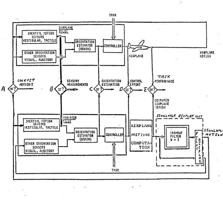
One possibility for quantifying realism is to use cockpit motions of the simulator as compared with those of the actual

air-craft (see Figure 1.8). This, however, would require an extremely expensive motion system or an in-flight simulator such one described in 1.1. Another possibility is using an "orientation estimate" which the central nervous system estimate of the motion after pro-cessing signals from the vestibular as well as the visual, tactile, auditory and other sensory systems. Although research is currently being done to find out more about the interaction of these systems, not enough is currently known to apply this method.

AIRP LANE INERTI.\l lTori SENSORS VESTIBULARITACTILE _ORIENTATION ESTIMATOR EN SO(BRAIh) OTHER ORIENTATION-SENSORS VISUAL.AUDITORY coc /r1' SENSORY

MOT IOI ONSEASUREMENTS

IMUO.A TO R fEATIAL MOTION Lg JESTI SE SrT ACS E- _~ YESTCULR. :ACILEORIE11TATION ESTIMATOR aCONTROL.LER. (ORAMN) -OTHER :alENTATION SENSCRS VISUAL, AU01T09Y TAS.. AIRPLANL COMPUTA-TIN -- 0---COMPUTED IMPLAXE '-.0T 10:1

STA( AT-rG _fQA*.r

.,:ASPOUT 5i 4 Lar

FILTER P A t

W . ?

L

~

rj

Figure 1.8: Comparison of ?ossible ''atching Points to Achieve Simulator nealism (Ish-Shaloa, 1982)

19 TAS K

7

-Lj--,,

Ish-Shalom (1982) used models of the vestibular system to quan-tify simulator realism for his optimal flight simulator design. The cost functional in this method is based on the difference

be-tween the physiological outputs of the vestibular system of a pilot in an imaginary reference airplane to those of the pilot in the simulator. This difference is defined to be the vestibular error.

Sullivan (1985) implemented an optimal washout system based on the vestibular error on the VMS and compared it to the motion control system normally used for this system. These systems were compared in terms of performance in a tracking task, Cooper-Harper handling quality ratings and simulator motion quality ratings given by pilot subjects. His experiments show that the use of vestibular models is a reasonable approach to the design and evaluation of motion control systems.

Because one of the primary goals of the simulation is to ade-quately train pilots, two other possible methods to acheive sim-ulator realism are matching pilot control effort and matching pilot performance for the simulator and the aircraft. A disadvantage to these methods is that it is not at all clear that just because the pilot is controlling the aircraft the same way or performance is measured to be the same that the simulation is realistic. A variety of different types of motions could cause the pilot to

execute the same control motion while the same performance can be achieved by vastly different strategies. More about all of these possibilities is discussed by Ish-Shalom (1982). Sullivan (1985) found that although performance is widely used as a simulator

fid-elity measure, it is not necessarily a valid or consistent measure.

1.5 This Research - More Basic Questions

As stated earlier, there is an implicit assumption that simu-lator motion is critical for realism and thus for the transfer of training from simulator to aircraft. Therefore, much effort has been put into the problem of how to best design controllers for

this motion in order to make the simulation realistic. A major problem with this research has been that it is not clear how to quantify simulator realism. Although some work has been done using

scientific knowledge of the human perceptual systems, many washout systems today are still being designed mainly by intuition.

This research will examine more basic questions than how to best control the motion of the simulator in order to make the flight realistic. The purpose of this thesis is to examine the

relation-ship between flight simulator motion and realism. This will be done by examining the effect of different levels of motion capabi-lity on various parameters of engineering, psychological, and physiological realism. The variables used to represent realism are vestibular errors and acceleration errors, as well as pilot opinion and performance measures. Vestibular error is primarily a physiological fidelity measure; acceleration error, an engineering fidelity measure, and opinion, a psychological measure. Because these measures are not independent, it will important to look for consistencies or inconsistencies in what they show. There is not really a good reason to classify performance as a realism measure.

As mentioned before different control strategies can achieve the same performance, so similar performance does not necessarily sig-nify realism. However, because difference in performance could signify lack of realism, it will be helpful to examine performance measures in addition more direct realism measurements.

Three different motion conditions were used to represent the spectrum of motion capability. For the lowest fidelity motion condition, the simulator only consisted of special effects motions like turbulence. The amplitude of these motions was small compared to the other conditions. In the "jostle" motion condition, the simulator was allowed to move in only two directions -- lateral and longitudinal translational. Special effects were also included in this condition. The last motion condition allowed motion in all six degrees of freedom. Special effects were included in this condition also.

Experiments, which are described more fully in the next chap-ter, were performed on a Boeing 727-200 simulator located at NASA Ames. Flight scenarios were chosen that were representative of

the training environment. These manuevers required significant pilot control activity so that motion platform effects, if they

existed, and could be measured this way, were as detectable as possible. The three flight scenarios chosen were engine flameout

on takeoff, an airwork scenario, and an ILS approach and landing windshear scenario. The airwork scenario consisted of steep turns, approach-to-stall manuevers and standard rate turns with a yaw damper failure. The effect of motion on pilot vestibular error,

opinion and performance is relevant to all types of washout system design methodologies, not just the optimal control methodology.

1.6 Thesis Outline

This thesis is organized as follows. Chapter 1 is a general introduction to flight simulator technology and the problems that are examined in this thesis. The vestibular models are formulated in chapter 2. Chapter 3 is a detailed description of the experiment methodology issues. Opinion results are are presented and discussed in chapter 4. Acceleration error results are presented and disc-ussed in chapter 5. The vestibular error results are located in chapter 6. Chapter 7 is a presentation of the performance results. Chapter 8 is a discussion about the problems that occurred due to undersampling of the data. Chapter 9 deals with conclusions and suggestions for further research.

CHAPTER 2: FORMURATION OF THE VESTIBULAR ERROR AS A MOTION FIDELITY

2.1 Introduction

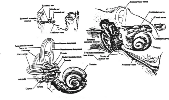
In the absence of visual cues, the vestibular system is the primary physiological system used to detect motion. The vestibular system consists of the semicircular canals, which detect rotational accelerations and the otoliths, which detect translational motion

(see Figures 2.1 and 2.2). The vestibular system is particularly good at detecting high frequency motion, while the visual system perceives strong motion cues from low frequency motions especially in the peripheral field-of-view. This report focuses solely on the vestibular system because it is not clear how the two systems int-eract. Also because of the limited travel of the simulator, motion that is simulated is primarily high frequency motion.

This chapter is a description of the vestibular system. Mathe-matical models of the semicircular circular canals and otoliths are presented, and the concept of vestibular error is introduced.

2.2 Semicircular Canals

2.2.1 Physical Description of the Semicircular canals

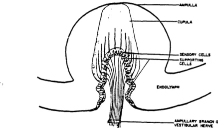
The semicircular canals are used to sense rotational motion with respect to inertial space. There are three approximately orthogonal canals which are filled with a fluid called endolymph. When the head rotates with respect to inertial space the endolymph, due to its inertia, initially tends to remain fixed. The semicircular canals, which form approximately two thirds of a circle, have an expanded

section at the base called the ampulla, which leads into a common base called the utricle (see Figures 2.3, 2.4, and 2.5). The ampulla

is blocked by the cupula. When the water-like endolymph moves rela-tive to the canals, which is the end result of the fluids initial tendency to stay fixed in inertial space, sensory hair cells embedded in the base of the cupula are bent. By increasing their firing

frequency, these hair cells provide information about the motion to the central nervous system. The hair cells in a particular semicircular canal are all polarized for sensing motion in the same direction. So each canal is used for a particular direction. Theoretically, by combinations of the information provided by the

three orthogonal canals, the CNS can detect motion in any direction. There are two types of hair cells in the canals - type I and type II (see Figure 2.6). Type I cells, which have an irregular dis-charge pattern in the afferents and show adaptation, may be sensitive to both hairbendings and the rate of change of hairbendings (Hosman and Van der Vaart, 1978). Type II hair cells are believed to pri-marily sense hair bendings.

2.2.2 Mathematical Model of the semicircular canals

The endolymph is acted on by primarily two forces. The first is viscous drag, which is the proportional rate of velocity of the fluid with respect to the walls of the canal. The second is modelled as a linear elastic restoring force that is caused by the cupula's tendency to return to its resting position. The equations below represent a basic but incomplete model of a canal and were first proposed by Steinhausen in the 1930's (Ormsby, 1974 ).

as I#

m(ec + eci) - -V 8ec -k eec

9ec

eci - angular position of canal with respect to inertial space m - moment of inertia of endolymph

V - coefficient of viscous drag

k - coefficient of linear restoring force due to displacement of fluid in the canal

The system appears to be overdamped and k/V << V/m this equation can be approximated as:

ec(s)i)-l

c i(s )(s+k/V) (s+V/m)

This model is called the overdamped torsional pendulum model. Recent efforts have included a lead term to represent the sensitivity of type I haircells to the rate of cupula displacement. Based on studies of the squirrel monkey, Fernandez and Goldberg (1976) estimated

the lead time constant to be 0.049 sec. Another addition to the basic torsional pendulum model has been included because adaptation to prolonged accelerations was noticed. Adaptation could be due to processing by the CNS; or it could be attributed to adaptation in the sensory haircells; or it could be a combination of these effects. The adaptation term, which is due to the efforts of Young and Oman (1969), causes a phase lead and gain attenuation at low frequencies. In any case the full transfer function which now relates spatial orientation to angular acceleration of the head for one degree of freedom can now be written as:

H(s) - Gscc . Tas (l+TLs) (1+Tas) _(1+Tls)(l+T

2s)

The output is measured in threshold units so that a response of one is obtained for a sinusoidal input of amplitude 1.450/sec2 and frequency of 0.94 rad/sec as found by Hosman and Van der Vaart (1978), who also obtained T1 -5.9 sec. The adaptation term has a

value of Ta- 80 sec (Young and Oman, 1969). T₂ has such a high frequency that is difficult to measure. Theoretical estimates by Steer (1967) estimate this value to be 0.005 sec (Hosman and Van der Vaart, 1978). Bode plots are shown in Figure 2.7.

In this report, this model is limited by the sampling rate of the flight simulator computer, which was 30 times per second, so the highest frequency in the model should be 15 Hz. Therefore, to prevent undersampling, the lead term and the high frequency pole, with frequencies of 20.4 hz and 200 hz rspectively, have been elim-inated. In this report, the following transfer function was used to represent a semicircular canal:

H(s) - Gscc . Tas . I

(1+Tas) (1+Tls)

Gscc - 222.7 sec2/rad Ta - 80 sec

Tj - 5.9 sec

This transfer function is used for each of the three degrees of freedom. Bode plots are shown in Figure 2.8.

M~t~ZU

Figre _{.1 Th stucureoftheinnr ar.(Peeram169}

I

~

0

0

Figure 2.2 Orientation of the seimicircuiir canals and the otoliths with respect to the head

Ampulla Cr isto Membranous Horizontal Semicircular Canal 1.1 mm Utricle 6.4 rmm 0.24 mm

Figure 2.3: Average dimensions of Semicircular Canali (Peters,1969) x y Superior Canals Utricles Right

Vectoril indicate Horizontal Canal effective direction of

angular .cceleration Left

Coa l _{Posterior Canals}

Fi&LARE2,41

The effective directions of the semicircular canals (approximate) (Peters,1969)

-SENSORY CELLS

Type I

~fL

Figure 2.5: Simplified diagram of ampulla section of semicircular canal (Peters, 1969)

heir mm

_S

_O*

Efend., n * r VA b

Figure 2.6: Schematic drawing of type i and type I Hair cells

k

I

C

1s)(rice

I

oL

(de

vee")

--100.'

SEMICIRCULAR CANAL MODEL FREQUENCY RESPONSE PLOTS

MAGNITUDE

_/Sec

Figure 2.7: Frequency Response Plots of Semicircular Canal Model

...

so.[

-So.

4

SCC MODEL

FREQUENCY RESPONSE

10

50.

-o..

-100.,

Figure 2.8 Frequency Response Plots of Semicircular Canal Model Used in this Report.

2.3 Otoliths

2.3.1 Physical Description

The otolith organs, also located in the inner ear, are used to detect translational accelerations. This includes gravity, which

is a translational acceleration of 9.8 m/sec2. There are two oto-lith organs located in each inner ear. One of them is located in the utricle, which is the common base of the semicircular canals. The other otolith organ is located in the saccule, which is a downward extension of the utricle. The basic structure of the otolith con-sists of a supporting base called the macula (Figure 2.9). Covering the macula is a gelatinous layer containing suspended calcite crys-tals. When the head is exposed to a specific force, the calcite crystals have more inertia than the gelatinous layer, and the layer shears. Sensory haircells embedded in the macula are bent and a signal is sent to the central nervous system. The otoliths have the same two basic types of haircells that are located in the semi-circular canals; however, unlike the canals, hairs in one organ are polarized in different directions. This enables motion sensa-tion in the three degrees of freedom when there are only organs in two approximately orthogonal directions.

2.3.2 Mathematical Models of the Otoliths

An otolith organ can be modelled as a overdamped spring-mass-damper system with the following transfer function, which describes translational acceleration perception to specific force.

H(s) - K

(l+T₃s)(l+T_4s)

Modifications proposed by Young and Meiry (1968) include a lead term which takes into account adaptation.

H(s) - K(1+Tns) (1+T₃s)(l+T_4s) Tn - 13.2 sec T3 - 5.3 sec T4 - .67 sec K - gain factor

In this report, approximations were made to prevent undersampling. The transfer function actually used was:

H(s) - Go(l+Tns) (l+T_3s)

Go - 2.13 sec2/m Tn - 13.2 sec T3- 5.3 sec

Threshold units were used to give a response of 1 when sub-jected to accelerations of 0.47 m/sec2 as discovered by Hosman and Van der Vaart (1978). Figure 2.10 shows other experimental estimates of the threshold level of perception. In this report, all degrees of freedom are represented by this model. Bode plots for one degree of freedom are shown in Figure 2.11.

Time constants in the otolith model are not as definite as in the semicircular canals. This is partly because of difficulties in the experimental tools used. For semicircular canal research, subjective experiments can be performed in a rotating chair with

well-trained subjects. For otolith research, a smoothly running translational car is needed (Hosman and Van der Vaart, 1978).

2.4 Vestibular Error Measurements

Based on the vestibular models described above, one can cal-culate a response in threshold units. Because the simulator under-goes different accelerations than the actual airplane, the simulator vestibular response will be different from the vestibular response that would occur in an actual aircraft (see Figure 2.12). The dif-ference in these two responses is defined as the vestibular error. The input accelerations to the vestibular must be in cockpit body axis coordinates.

Because it was desired to compare average magnitudes of these errors and not to compare functionality, a root mean square error was computed for specific data windows of interest. This measure will be discussed further in Chapter 3.

STATOCONIm

GEAT:..NOW '~v

100 50 33 25 171 PERIOD, SECONDS 10 5 3.3 2 1 0.5 0.25 0.17 0.1 0 05 ooZ 0.1 0.08 0.06 0.04 Table 2.1 SOURCE Chaney 1(4) Chaney 1(5) Chen and Robertson 3 Chen and Robertson 3 Goril and Snyder 1(8) Gurney 1(12) Landsberg 1(18) Richer and Meister 1(22) von Bekesy 2 Walsh 1(24) Walsh 1(26) Benson Bionetics at Miami U.4 TEST RIG Vertical Axis Shi

Vertical Axis Sh Closed room on a platform with 2-. horizontal motio Closed room on a pendulum Vertical Axis Sh Vertical circula 3.26m radius 3.6m Pendulum Platform drivenI eccentric mass vibrator 2m Horizontal circular arc 1.55m Pendulum Vertical circula Vertical hydraul driven oscillato 4m Pendulum

SUIARY OF THPESHOLD-OF-PERCEPTI ON DATA SOURCES (from fig. 2.10)

(-r~gAB ci, \9 ACCELERATI DIRECTIONS TEST SUBJECTS/ACCOMMODATIONS TEST SUBJE aker 10 males, seated with lap belt restraint and footrests. Z-Z

Each subject makes 4 determinations at 4 frequencies

(8 measurements for each frequency data point).

aker 5 males, standing, feet attached to moving platform. Z-Z

2 subjects at each frequency, standing. 3 X-X

axis 4 Y-Y

on

25m 10 subjects sitting. 5 X-X

10 subjects sitting. 6 Y-Y

20 subjects standing. 7 X-X

aker 6 males (air crew) seated in a cockpit simulation. Z-Z r are 3 subjects sitting blindfolded (seesaw). . Z-Z

Subjects lay face-down and face-up. Z-Z by 10 subjects in five positions; Standing, X-X, Z-Z; 11, All

lay face-up X-X, Y-Y, Z-Z. (12 is X-X face up only.) 12, X-X

2 subjects seated y-y

4 to 7 subjects each test point. Lay face-up, face- 14, X-X down, on sides. 8 measurements for each subject. 15, Y-Y

16, Z-Z

r arc 7 males, 4 measurements each, 8 times. Lay face-up. X-X ic _{6 males, 4 females in an aircraft ejection seat. Z-Z}

r-2 males lay face-down, series of measurements at one Y-Y frequency. . . F I iI _{I 2} - --p 3 (06 3 4 1116 04:4p 0.006 0.01 0.02 0.04 0.06 0.1 0.2 0.4 0.6 1.0 2 3 4 5 6 8 10 20 40 60 80 FREQUENCY, Hz

Fig ure,.-2 .10 Threshold-of-Pe'rception Measurements and a Design Limit ror

Spurious Accelerations -- (Taback 1983) Nd . L-CD --0.02 0.01 0.005 0.003 0.001 0.008 0.006 0.004 0.002 0.0007 0.0005 0.0003 DATA POINT 1 2 3 4 5 6 7 8 9 10 11 12 13 14 15 16 17 18 19

OTOL ITN FPGQUgw-E Malj It-

1-'

10

p .t

10~1

Figure 2.11: _{Otolith Model freouency response plots} 1' lou w C.raA/,A..

100

10

0~4

TAWLATIOUAL VZSTISULAA Eacas t ROTATIONAL ACCELEZATION MDELLED AIRCRAFT TRANSLATIONAL MDEL Or

ACCELEXATIONS OTOLIN ORCAN

MDELLED AIRCRAFT

ROTATIONAL MDEL Or SEMICIACULA"

ACCELERATIONS CANAL ORGAN

SIMULATOR

TRANSLATIONAL MOEL OF OTULITN

ACCELERATIONS ORGAN SIMULAroft

ACCgLUT ONS MODEL OF SEMICIRCULAR

CANAL OR.AN

Figure 2.12: Calculation of Vestibular Error

CHAPTER 3: EXPERIMENTAL DESIGN AND ANALYSIS MEASUREMENTS

3.1 Brief Introduction

This chapter is a summary of the experimental procedure. A description of the experiments is presented first and is divided

into sections about the simulator, motion conditions, flight scen-arios, subjects, and order effects. The second part of this chapter discusses the actual measurements taken and and the third section is a discussion of data collection.

3.2. Experiment Description 3.2.1 Simulator

Experiments were performed with a Boeing 727-200 series flight simulator on a six degree of freedom synergistic motion base. It uses a nonlinear adaptive washout system. The visual system used for this study is a computer-generated dusk/twilight scene. This simulator meets the requirements for Phase II certification under Federal Aviation Regulations. The simulator, which is designed by the Singer-Link company, is located at the NASA Ames Research Center. Figure 3.1 is a picture of the actual aircraft.

3.2.2 Motion Conditions

Three motion conditions were used. In the "fixed-base" con-dition, only special effects motion was allowed. Special effects included runway touchdown bumps, vibrations due to the roughness of

*O-rr

i dw.

the runway, buffets associated with flap, gear and spoiler exten-sion, turbulence, and Mach and stall buffet. The special effects only motion condition is the most severely limited condition in the

study. The amplitude of these vibrations is small compared to the motion capabilities in the other conditions. "Jostle " motion

condition provided only two degrees of freedom: vertical transla-tional and lateral translatransla-tional. This condition, which also in-clude all of the special effects mentioned above, was inin-cluded to study the effects of providing mostly translational acceleration information to the pilot. The last motion condition, full motion, provided full six degree of freedom capabilities as well as the special effects included in the other conditions. This condition is the nominal condition for the simulator.

3.2.3 Flight Scenarios

The environmental data base used in the simulations was the area of the San Francisco International Airport. The aircraft takeoff weight was set to 148000 lbs. Although flights were short so the fuel burn that would occur is slight, the weight was held constant throughout the experiments in order to eliminate the effects of weight changes due to fuel burn which might vary due to different piloting techniques. All scenarios, with the exception of the ILS Approach and Landing Scenario, were conducted in the

standard day (pressure - 1 atm, temperature- 150 C) with no wind and good visibility.

3.2.3.1 Familiarization Scenario

This scenario was flown by all subjects directly before begin-ning their series of experimental flight scenarios. The purpose of this scenario was to allow the pilots to get used to the simu-lator. Because the purpose of this study was to compare solely the effects of motion fidelity levels on a variety of parameters, allowing the subjects to become familiar with the simulator hope-fully reduced the possible learning effects. (In similar experi-ments Sullivan (1985) found learning effects on some performance measures.)

A familiarization scenario run began at the departure end of runway 28R at the San Francisco International Airport. The pilots followed air traffic control vectors around the traffic pattern for a visual approach to a touch-and-go landing. The subject then followed the vectors around the traffic pattern for another visual approach to a full stop landing. Subjects then had the choice of performing this scenario again.

3.2.3.2 Engine flame-out on takeoff

This scenario began with the aircraft ready for takeoff at the end of runway 28R of the San Francisco International Airport. The subject was informed in advance that there would be an engine flame out in one of the off-centerline engines (#1 or #3). At the beginning of each run, the experimenter randomly chose which engine would fail. Randomization was used to prevent the subject from making anticipatory control motions. The time of engine failure was also varied but always occurred within five seconds following

rotation, that is beyond V2. The engine flameout occured after V2 so that the pilots could not decide to abort the takeoff. Subjects were instructed to maintain runway heading and level out at an altitude of 2000 ft.

3.2.3.3 Airwork Scenario

The Airwork Scenario, run began with the aircraft at 15000 ft with 250 knots indicated airspeed directly above the San Francisco International Airport with a heading of 2800. The pilot was in-structed to perform two consecutive steep turns 450 bank, one to the right and one to the left, to make one "s" turn, two approach-to-stall manuevers, and then two standard rate turns with the yaw dampers failed.

3.2.3.4 ILS ADproach and Landing Scenario

Pilots flying the ILS Approach and Landing scenario were ini-tialized at an altitude of 4000 ft, an airspeed of 220 knots indi-cated airspeed, and an intercept course of 300 off the localizer to SFO's runway 28R. The simulator was set for moderate turbulence levels. There was 600 ft ceiling and unlimited visibility at 500 ft. A windshear, described in Figure 3.2, was introduced at this altitude. Pilots were instructed to land the aircraft and were informed of the presence of windshear.

5 kts 0Okts 5 kts

WINDSPEED (K-+S)

FIGURE 3.2: WINDSHEAR MODEL (Arrow-3iindcult

to incm

FOR ILS APPROACH AND LANDING SCENARIO

direci.on

of

oircraf+).

ALTTUDE

3.2.4 SubJects

Eighteen air transport pilots were used in the study.

The subjects were told that the experiment was a study on flight simulator fidelity. They were not told before the experiment that the experimental conditions would vary only the motion platform capabilities. Briefing material given to the pilots before the experiments is located in the Appendices.

The primary subject chose his preferred seat, left or right and flew as pilot-in-command, and the secondary subject flew second-in-command. Data was taken on the first subject and then the levels of command were switched, the new subject chose his seat and data was recorded again. Due to schedule changes, the second-in-command seat was sometimes taken by a non-subject pilot. To minimize the effect on exposure to another subject's experiment which might induce learning effects, subjects who flew in groups of two were given different flight scnearios to perform.

The eighteen pilots were randomly divided into groups of three so that six subjects flew each of the three flight scenarios. Pilots 4, 6, 7, 12, 16, and 18 performed the ILS Approach and

Landing in wind shear scenario. Pilots 2, 5, 10, 11, 14, and 17 performed the engine-flame out scenario, and pilots 1, 3, 8, 9, 13, 15 performed the airwork scenario. Before performing the actual experiments, all subjects flew the familiarization scenario which consisted of VFR takeoffs, approaches and landings.