Dynamic shortest paths algorithms : parallel implementations and application to the solution of dynamic traffic assignment models

(1)

/6

Dynamic Shortest Paths Algorithms: Parallel

Implementations and Application to the Solution

of Dynamic Traffic Assignment Models

by

SRIDEVI V. GANUGAPATI

B.Tech., Indian Institute of Technology, Madras (1996)

Submitted to the Department of Civil and Environmental Engineering

in partial fulfillment of the requirements for the degree of

Master of Science in Transportation Engineering

at the

MASSACHUSETTS INSTITUTE OF TECHNOLOGY

June 1998

@

Massachusetts Institute of Technology 1998. All rights reserved.

Author ...

.. .

Department of

.... Civil..

Civil .an

Environmental Engineering

May 22, 1998

Certified by...

/

Assistant Professor

Ismail Chabini

Thesis Supervisor

Accepted by... ...

..

...

Joseph M. Sussman

Chairman, Department Committee on Graduate Students

(2)

Dynamic Shortest Paths Algorithms: Parallel

Implementations and Application to the Solution of

Dynamic Traffic Assignment Models

by

SRIDEVI V. GANUGAPATI

Submitted to the Department of Civil and Environmental Engineering on May 22, 1998, in partial fulfillment of the

requirements for the degree of

Master of Science in Transportation Engineering

Abstract

Intelligent Transportation Systems (ITS) promise to improve the efficiency of the transportation networks by using advanced processing, control and communication technologies. The analysis and operation of these systems require a variety of models and algorithms. Dynamic shortest paths problems are fundamental problems in the solution of most of these models. ITS solution algorithms should run faster than real time in order for these systems to operate in real time. Optimal sequential dynamic shortest paths algorithms do not meet this requirement for real size networks. High performance computing offers an opportunity to speedup the computation of dynamic shortest path solution algorithms. The main goals of this thesis are (1) to develop parallel implementations of optimal sequential dynamic shortest paths algorithms and (2) to apply optimal sequential dynamic shortest paths algorithms to solve dynamic traffic assignment models that predict network conditions in support of ITS applications.

This thesis presents parallel implementations for two parallel computing plat-forms:(1) Distributed Memory and (2) Shared Memory. Two types of parallel codes are developed based on two libraries: PVM and Solaris Multithreading. Five de-composition dimensions are exploited: (1) destination, (2) origin, (3) departure time interval, (4) network topology and (5) data structure. Twenty two triples of (parallel computing platform, algorithm, decomposition dimension) computer implementations are analyzed and evaluated for large networks. Significant speedups of sequential al-gorithms are achieved, in particular, for shared memory platforms. Dynamic shortest path algorithms are integrated into the solution algorithms of dynamic traffic assign-ment models. An improved data structure to store paths is designed. This data structure promises to improve the efficiency of DTA algorithms implementations.

Thesis Supervisor: Ismail Chabini Title: Assistant Professor

(3)

Acknowledgements

I am immensely grateful to Professor Ismail Chabini for his guidance and encour-agement throughout the course of my study. I have benefitted a lot through the numerous research discussions we had in the past one and half years. The supervi-sion of Professor Ismail Chabini not only helped me grow intellectually but also as a student, skilled professional and most importantly as an educated person.

I also want to recognise and thank many of my colleagues at MIT for their assis-tance: Brian Dean for very useful discussions on shortest path algorithms and also for the computer codes on one-to-all dynamic shortest path problems, Parry Husbands and Fred Donovan for their assistance with the xolas machines, Yiyi He for the DTA codes, Qi Yang for his assistance with PVM, Jon Bottom for the discussions we had about path data structures.

I would like to thank my friends in CTS, particularly people in ITS and 5-008 offices for making me feel at home while at MIT.

I do not find enough words, when I want to thank my family, Amma, Daddy, Suri and Anil, for their love, affection and support. I owe everything to them.

(4)

I dedicate my work to my parents Rama and Hymavathi,

my sister Suri and my brother Anil.

(5)

List of Figures

2.1 _{Representation of a dynamic network using time space expansion .} ₂₃

2.2 Illustration of forward labeling for non-FIFO networks ... 30

2.3 Algorithms for FIFO networks ... 51

2.4 Algorithm IOT: varying maximum link travel time ... . . 52

2.5 Algorithm IOT: varying number of nodes ... . . . . 52

2.6 Algorithm IOT: varying number of links . ... 53

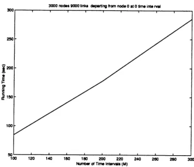
2.7 Algorithm IOT: varying number of time intervals ... 53

2.8 Algorithm IOT-MinCost: varying number of nodes . . . . 54

2.9 Algorithm IOT-MinCost: varying number of links . . . . 54

2.10 Algorithm IOT-MinCost: varying number of time intervals ... 55

2.11 Algorithm IOT-MinCost: varying maximum link travel time .... . 55

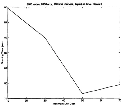
2.12 Algorithm IOT-MinCost: varying maximum link cost ... 56

2.13 Algorithm DOT: varying number of nodes) . ... . . . . 56

2.14 Algorithm DOT: varying number of links ... . .. . . . 57

2.15 Algorithm DOT: varying number of time intervals . . . . 57

2.16 Algorithm DOT-MinCost: varying number of nodes ... . . 58

2.17 Algorithm DOT-MinCost: varying number of links ... . . . . . 58

2.18 Algorithm DOT-MinCost: varying number of time intervals ... 59

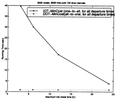
2.19 Comparison of algorithm IOT and algorithm DOT . . . . 59

2.20 Comparison of algorithm IOT-MinCost and algorithm DOT-MinCost . 60 3.1 Shared Memory System ... ₆₆

(11)

3.3 The Solaris Multithreaded Architecture (Courtesy: Berg and Lewis [24]) 77

4.1 Application Level Parallel Implementations ... ... . 89

4.2 Algorithm Level Parallel Implementations ... . ... 90

4.3 Illustration of implementation on a distributed memory platform of an application level (destination-based) decomposition strategy .... . 91

4.4 Illustration of implementation on a shared memory platform of an ap-plication level (destination-based) decomposition strategy . . . . 91

4.5 Illustration of Decomposition by Network Topology ... 92

4.6 Computing Minimum with a Complete Binary Tree ... 121

4.7 Decomposition by Destination(with collection of results by the master process in PVM implementations) ... . 128

4.8 Performance of (PVM, Destination, DOT Implementation: varying num-ber of nodes ... . 129

4.9 Performance of (PVM, Destination, DOT Implementation: varying num-ber of links .. ... .... .. ... .. .. .. ... .. .. .. . 129

4.10 Performance of (PVM, Destination, DOT Implementation: varying num-ber of time intervals ... . 130

4.11 Decomposition by Destination(without collection of results by the mas-ter process in PVM implementations) . . . 130

4.12 Decomposition by Origin (FIFO networks) . . . 131

4.13 Decomposition by Origin (non-FIFO networks) ... 131

4.14 Decomposition by Departure Time (FIFO networks) ... 132

4.15 Decomposition by Departure Time (non-FIFO networks) ... 132

4.16 Performance of (PVM (without collection of results by the master pro-cess), Destination, DOT) Implementation: varying number of nodes . . 133

4.17 Performance of (PVM (without collection of results by the master pro-cess), Destination, DOT) Implementation: varying number of links . . 133

(12)

4.18 Performance of (PVM (without collection of results by the master

pro-cess), Destination, DOT) Implementation: varying number of time in-tervals . . . 134 4.19 Performance of (MT, Destination, DOT) Implementation: varying

num-ber of nodes ... 134

4.20 Performance of (MT, Destination, DOT) Implementation: varying

num-ber of links . . . .. .. . . .. . . .. . .. .. .. ... . . . . 135

4.21 Performance of (MT, Destination, DOT) Implementation: varying

num-ber of time intervals ... .... 135

4.22 Performance of (PVM, origin, lc-dequeue) Implementation: varying

number of nodes ... _.. ₁₃₆

number of links ... ₁₃₆

number of time intervals ... ... 137

4.25 Performance of (PVM, origin, IOT) Implementation: varying number

of nodes ... ₁₃₇

of links . .. .. .. . . . .. . . . .. .. . . . .. . . . ... 138

of time intervals ... ₁₃₈

4.28 Performance of (MT, origin, 1c-dequeue) Implementation: varying

number of nodes ... ... . 139

4.29 Performance of (MT, origin, Ic-dequeue) Implementation: varying

number of links ... ₁₃₉

4.30 Performance of (MT, origin, 1c-dequeue) Implementation: varying

number of time intervals ... 140

4.31 Performance of (MT, origin, IOT) Implementation: varying number of

(13)

4.32 Performance of (MT, origin, IOT) Implementation: varying number of links . . . . 141 4.33 Performance of (MT, origin, IOT) Implementation: varying number of

time intervals ... 141 4.34 Performance of (PVM, Departure Time, lc-dequeue) Implementation:

varying number of nodes ... 142 4.35 Performance of (PVM, Departure Time, lc-dequeue) Implementation:

varying number of links ... 142 4.36 Performance of (PVM, Departure Time, lc-dequeue) Implementation:

varying number of time intervals ... 143 4.37 Performance of (PVM, Departure Time, IOT) Implementation: varying

number of nodes ... 143 4.38 Performance of (PVM, Departure Time, IOT) Implementation: varying

number of links ... 144 4.39 Performance of (PVM, Departure Time, IOT) Implementation: varying

number of time intervals ... 144 4.40 Performance of (MT, Departure Time, 1c-dequeue) Implementation:

varying number of nodes ... .. 145 4.41 Performance of (MT, Departure Time, lc-dequeue) Implementation:

varying number of links ... 145 4.42 Performance of (MT, Departure Time, lc-dequeue) Implementation:

varying number of time intervals ... 146 4.43 Performance of (MT, Departure Time, IOT) Implementation: varying

number of nodes ... 146 4.44 Performance of (MT, Departure Time, IOT) Implementation: varying

number of links ... ... 147 4.45 Performance of (MT, Departure Time, IOT) Implementation: varying

number of time intervals ... 147 4.46 Decomposition by Network Topology . ... 148

(14)

4.47 MT implementation of Decomposition by Network Topology of

algo-rithm DOT (Varying number of nodes) ... 148

4.48 MT implementation of Decomposition by Network Topology of algo-rithm DOT (Varying number of links) ... . . . . 149

4.49 MT implementation of Decomposition by Network Topology of algo-rithm DOT (Varying number of time intervals) . ... 149

5.1 _{A Framework for Dynamic Traffic Assignment Models ...} _{. . . .} ₁₅₄

5.2 A simple network to illustrate the subpath table data structure . . . 155

5.3 Algorithm INTEGRATE ... 159

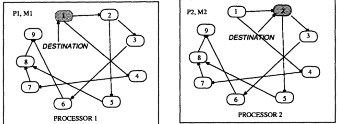
5.4 Test Network ... _{... ...} ₁₆₀

5.5 Amsterdam Beltway Network ... 167

5.6 Sub Path Tree for the network in Figure 5.4 . . . ... . . . 169

5.7 Updated Sub Path Tree for the network in Figure 5.4 ... 170

5.8 An extended sub path tree ... 171

A.1 Directory Structure ... 178

B.1 Flowchart of the Integration of Path Generation Module into Dynamic Traffic Assignment Software ... 182

(15)

List of Tables

5.1 The subpath table for the network shown in Figure 5.2 .... . . . . 155

5.2 Initial subpath table for the network in Figure 5.4 . . . 162 5.3 Updated subpath table for the network in Figure 5.4 . . . 163 5.4 Path Travel Times (minutes) for OD pair (1,9) before the path generation164 5.5 Path Travel Times (minutes) for OD pair (1,9) after the path generation 164 5.6 Path Flows for OD pair (1,9) before the path generation . . . 165 5.7 Path Flows for OD pair (1,9) after the path generation . . . 166

5.8 Performance measures before and after the path generation ... . 166

5.9 Performance of the time dependent path generation component on the

(16)

Chapter 1 Introduction

Today's transportation infrastructure is often associated with congestion, inefficiency, danger and pollution. Traffic congestion costs society a lost in productivity. One way to solve the problems associated with traffic systems is to construct more highways. This solution is increasingly more expensive and is not always feasible because of spatial and environmental limitations, especially in urban areas.

A new way to reduce congestion problems is to use the existing infrastructure more efficiently through better traffic management by equipping transportation systems with information technologies. This is known as Intelligent Transportation Systems (ITS). These systems are based on integrating advances in sensing, processing, control and communication technologies.

The two building blocks of ITS are Advanced Traffic Management Systems (ATMS) and Advanced Traveler Information Systems (ATIS). ATMS is expected to integrate management of various roadway functions, predict traffic congestion and provide al-ternative routing instructions to users and transit operators. Real time data will be collected and disseminated. Dynamic traffic control systems will respond in real time to changing traffic conditions. Incident detection is seen as a critical function of ATMS. ATIS involves providing data to travelers in their vehicle, in their home or at their place of work. Users can make their travel choices based on the information provided by ATIS.

(17)

models and algorithms. In order to meet the real-time operational requirement of ATIS/ATMS, such algorithms must run much faster than real time.

Dynamic shortest paths problems are fundamental problems in the solution of the network models that support ITS applications. These shortest path problems are dif-ferent from the conventional static shortest paths problems since in ITS applications, networks are dynamic. Optimal sequential dynamic shortest paths algorithms do not compute dynamic shortest paths fast enough for ITS applications. High performance computing gives an opportunity to speedup the computation of these algorithms. In this thesis, we design, develop and evaluate various parallel implementations of dynamic shortest path algorithms.

Dynamic Traffic Assignment (DTA) models are used to predict network conditions to support ITS applications. Dynamic shortest paths algorithms are required to opti-mally solve DTA models. In this thesis, we apply dynamic shortest paths algorithms to the solution of analytical formulations of dynamic traffic assignment problems.

1.1 Research Objectives

The goals of this thesis are:

* to review optimal sequential dynamic shortest path algorithms and to report on the experimental evaluation of efficient computer implementations of these algorithms,

* to develop parallel implementations of optimal sequential dynamic shortest paths algorithms,

* to apply the dynamic shortest paths algorithms to the solution of analytical dynamic traffic assignment problems.

(18)

1.2 Thesis Organization

The rest of this thesis is organized as follows. Chapter 2 presents formulations, algorithms and experimental evaluations of sequential computer implementations for dynamic shortest path problems. Chapter 3 introduces parallel computation concepts required to develop the parallel implementations. Chapter 4 presents twenty two parallel implementations of optimal sequential dynamic shortest path algorithms. Chapter 5 describes the application of algorithm DOT to the solution of analytical formulations of DTA models developed by Chabini and He [8]. Chapter 6 summarizes the main conclusions of this research and suggests some directions for future research.

(19)

Chapter 2 Dynamic Shortest Paths

-Formulations, Algorithms and

Implementations

Shortest path problems have been studied extensively in the literature for many years due to their importance in many engineering and scientific fields. With the advent of Intelligent Transportation Systems (ITS), a class of the shortest path problems has become important. These are known as dynamic shortest path problems. In these problems, the travel time of the link varies with starting time on the link. This varying travel time adds a new dimension to the shortest path problems, thus, increasing their complexity.

Dynamic shortest path problem has been first proposed by Cooke and Halsey [12] about 30 years ago. Recently, Chabini [10] solved one of the variants of this problem by proposing an optimal algorithm, that is, no other algorithm with a better running time complexity can be found.

In this chapter, we present the formulations, efficient algorithms and an extensive evaluation of dynamic shortest path problems, relevant to traffic networks with the following objectives:

(20)

problems since these problems are critical in many transportation applications. * To demonstrate that these sequential optimal algorithrms do not solve realis-tic dynamic shortest path problems fast enough for Intelligent Transportation Systems applications. We will then conclude that an application of high perfor-mance computing is essential for solving realistic dynamic shortest path prob-lems in real time.

This chapter is organized as follows: In Section 2.1, we develop a classification of dynamic shortest path problems. This classification is important to formulate these problems and to develop solution algorithms and computer implementations for them. In Section 2.2, we present a representation of the network using a time-space expan-sion. This representation is useful in presenting certain properties of the dynamic networks. These properties will be used to develop efficient solution algorithms. In Section 2.3, we define the notation used in formulations and algorithms of dynamic shortest path problems. Sections 2.4 through 2.9 are the crux of this chapter. In these sections, we present the formulations and algorithms for different variants of the dynamic shortest problems. In Section 2.10, we present an extensive experimental evaluation of the computer implementations of the dynamic shortest path algorithms discussed in this chapter. Finally, Section 2.11 summarizes the conclusions of this chapter and motivates the need for parallel implementations of dynamic shortest path problems.

2.1 Classification

Dynamic shortest path problems can be classified into many types. This classification is important for formulations and solution algorithms of these problems. Chabini [10] presents the following classification of the dynamic shortest path problems:

* Minimum time vs. Minimum cost: This classification is based on the minimization criterion. For minimum-time problems, one wishes to find the

(21)

least travel time between a pair of nodes in the network. For minimum cost problems, a path with the least cost is desired.

* Discrete vs. Continuous time networks: This classification is based on how time is represented. For discrete time networks, time is represented in discrete intervals. The link travel times and costs within this interval are assumed to be constant. A discrete dynamic network can alternatively be viewed as a static network, using a time-space expansion representation (see Figure 2.2). This idea is further discussed in Section 2.2.

* Integer valued vs. real valued link travel times: In integer time networks, travel times are assumed as positive integers. In real-valued time networks, travel times can take real values.

* FIFO vs non-FIFO networks: First-In-First-Out (FIFO) networks are those in which it is ensured that a vehicle entering a link earlier than another vehicle will leave that link earlier. It is also referred to as the no-overtaking condition.

A mathematical definition of the FIFO condition is given in a later section.

This condition may be used to develop efficient algorithms for certain dynamic shortest path problems.

* Waiting is allowed vs waiting is not allowed at nodes: Unlimited waiting or limited waiting may be permitted at all the nodes or at a subset of nodes in a network.

* Type of shortest paths questions asked: The models and algorithms de-pend on the kind of shortest paths questions asked. For instance, one may want to determine shortest paths from one origin node to all the nodes in the network or from all the nodes to one destination node, for one departure time interval or for many departure time intervals. These basic problems can be extended to many-to-all or all-to-many problems.

The following two dynamic shortest path questions are most relevant for trans-portation applications:

(22)

- Question 1: What are the shortest paths from one origin node to all the other nodes in the network departing the origin node at a given instant, say 0?

- Question 2: What are the shortest paths from all nodes to a destination

node in the network, for all departure times?

Some of the work published in the area of dynamic shortest paths has dealt with Question 1 ( [15], [23], [25]) and some with Question 2 ( [12], [30], [10]). Algorithms that answer Question 1 or Question 2 can be used for a specific problem. One such specific problem is a dynamic shortest path problem in a traffic network. For traffic problems, we will demonstrate that algorithms that answer Question 2 are more efficient.

Most transportation problems need shortest paths from all nodes to many desti-nations in the network. For instance, Let us assume that algorithm algl answers Question 1 and that alg2 answers Question 2. A typical traffic network can have approximately 3000 nodes, 9000 arcs and about 300 destinations. If the time frame is discretized into 100 time intervals, then 100 iterations of algl will be

10 times slower than alg2 for this network (as will be seen in Section 2.10). In the following section, we describe a way of representing dynamic networks, which helps us present certain properties of the dynamic networks, which are useful in developing efficient algorithms. These properties can be used to develop efficient algorithms.

2.2 _{Representation of a Dynamic Network Using}

Time Space Expansion

A discrete dynamic network can be represented as a static network using a time space expansion. The time space expansion representation helps us understand certain properties of the dynamic networks for example, the acyclic property of the dynamic network along the time dimension.

(23)

Travel times

r- ---- Link in the static part

(1, 2 (3, 2, 1) t =3) dynamic network /3 Travel times 1 2 3 4 after 1 4 2 t = 2 are static t=1 12 4 (2, 2, 3) 1 3 Node at t = t=O 1 2 3..-t : Time interval Node

(a) Dynamic Network (b) Time-space Expansion

Figure 2.1: Representation of a dynamic network using time space expansion Figure 2.1 illustrates this representation for a small dynamic network. Figure 2.1a, shows a small dynamic network with 4 nodes, 4 links and 3 time intervals. The numbers on the links denote the travel times of the link for each time interval. For instance, (1, 1, 3) on link (3, _{4) denote that the travel time on link}(3, 4) 1 at time interval 0, 1 at time interval 1 and at time interval 2 is 3. The time-space expanded representation of this dynamic network is shown in Figure 2.1b. In this representation, each node in the dynamic network is represented as 4 copies, one at each time interval. Each row in the Figure 2.lb represents one time interval. In the dynamic network, the travel times are assumed to be static after 3 time intervals, hence the nodes at time interval t = 2 can be considered as extending to infinity. Each link in the dynamic network is also represented by four copies in the time-space expanded network, but in this representation, the links connect nodes at different time intervals. For example, one copy of the link between nodes 1 and 2 in the dynamic network with a travel time of 1 at time interval 0 is the link connecting node 1 at time interval 0 and node 2 at time interval 1. This shows that if we start at node 1 at time interval 0, we will reach node 2 at time interval 1.

A static shortest path algorithm can be applied on the network shown in Fig-ure 2.1b to compute dynamic shortest paths in the network shown in FigFig-ure 2.1a.

(24)

This will be inefficient because the static shortest path algorithm will compute short-est paths labels for all nodes at all time intervals (Recall that these nodes are just copies of the node in the dynamic network). Hence, we need to find the minimum over all time intervals, for each node.

In the next section, we present the notation used in the formulations and algo-rithms for dynamic shortest path problems presented in this chapter.

2.3 Definitions and Notation

Let G = (N, A, D, C) be a directed network where N = {1, ..., n} is the set of nodes,

A = _{{(i,j)li E N,j E N} is the set of links (or arcs). Let t be an index to an}

interval of time. We denote by D = {dij(t) (i,j) E A}, the set of time dependent

link travel times and by C = {cj (t) I(i, j) E A}, the set of time dependent link travel costs. Functions dij(t) are assumed to have integer valued domain and range. The functions dij(t) are assumed to take a static value after M time intervals. Hence, t

can take values from 0 to M - 1. Functions cij(t) have integer valued domain and

real valued range. cij(t) are assumed to be static when departure time is greater than or equal to M - _{1. We denote by B(i), the set of nodes having an outgoing arc into}

i, B(i) = _{{j E N(j, i) E A}. Let A(i) denote the set of nodes having an incoming}

are from i.

Arc travel times can possess a property called FIFO (or no-overtaking) condition ([23]). This condition may be useful in developing algorithms for certain dynamic shortest path problems. The FIFO condition can be defined mathematically in various forms. For instance, FIFO condition is valid if and only if the following system of inequalities hold:

t + dii(t) < (t + 1) + di(t + 1), V(i, j, t) (2.1)

Intuitively, it can be seen that this condition holds if no overtaking takes place. If the link travel times of a link in the network satisfy the above condition, that link

(25)

is called a FIFO link. If all the links in the network satisfy the FIFO condition, the network is called a FIFO network, else, it is called a non-FIFO network. When the FIFO condition is not satisfied, it may be preferable to wait at the beginning of the link before traveling on the link.

In non-FIFO networks, if waiting is not allowed, we can have shortest paths with loops (which simulate waiting at the nodes). Therefore, two waiting policies need to

be considered: waiting is allowed at nodes and waiting is not allowed at nodes.

In the rest of the chapter, we present formulations, algorithms and evaluation of computer implementations for two main dynamic shortest path problems: dynamic fastest path problems and dynamic minimum cost path problems. The two main questions discussed in each of these classes of problems are:

* Determine the dynamic fastest paths or minimum cost paths from one origin node in the network to all the nodes in the network for a given departure time at the origin node?

* Determine the dynamic fastest paths or minimum cost paths from all the nodes in the network to one destination node in the network for all departure time intervals?

For both these questions, we consider two kinds of dynamic networks: FIFO and non-FIFO. For each of these types of networks, we consider two kinds of waiting policies: unlimited waiting is allowed at all nodes and waiting is forbidden at all nodes.

2.4 _{One to All Fastest Paths for One Departure}

Time in FIFO Networks when Waiting is

For-bidden at All Nodes

This is the most studied version of the dynamic shortest paths problem ([12], [15],

(26)

algorithm can be generalized to solve the time dependent fastest path problem with the same time complexity as the static shortest paths problem. Dreyfus [15] was the first

to present this generalization heuristically. He concluded that Dijkstra's algorithm can be adapted to solve the dynamic shortest path problem. Later, Ahn and Shin [1] and Kaufman and Smith [23] and a few others proved that this generalization is valid only if the FIFO condition is valid.

Chabini [10] gives an intuitive and simple proof of the generalization of the results, as opposed to a lengthy proof given by earlier authors. These are obtained from a formulation of the problem. These are presented in the next subsection.

2.4.1 Formulation

Let fj denote the minimum travel time from origin node s to node j leaving the origin node at a given time interval to. To write the Bellman's optimality conditions for node j, we need to consider only the paths arriving at node i E B(j) at a time greater or equal to fi. Minimum travel times can then be defined as solution of the following set of equations:

minmm mmin (t+dij (t)) , j 0 o

f

= iEB(j) t>fi, (2.2)

0 _,j=o

Proposition 1 If the FIFO condition is satisfied, the above formulation of the fastest

paths problem is equivalent to the following equations :

min (fi +di (fi)) , j o

fj = iEB(j) _(2.3)

0 _,j=o

Proof: The equivalence holds because, min(t + dij(t)) = fi + dij(fi), if the FIFO

tfcondition holds (see equation 2.1).

(27)

The equivalent formulation in equation 2.3 is similar to static shortest paths

opti-mality conditions with t replaced by fi. _{Hence, it shows that all static shortest paths}

algorithms can be extended, without any extra execution time, to solve the fastest paths problem if the FIFO condition is satisfied. Chabini ([10]) also notes that only a static forward labeling process can be used. We summarize this result in the following proposition.

Proposition 2 If the FIFO condition is satisfied, the formulation of the fastest paths problem in dynamic networks is equivalent to a static shortest paths problem. Hence,

any forward labeling static shortest path algorithm can be used to solve the dynamic fastest paths problem. The dynamic fastest problem is solved in the same time com-plexity as the static shortest paths problem.

Based on the above results, three different forward labeling algorithms/ imple-mentations are designed: label setting algorithm with heaps (Dijkstra's algorithm [13], label setting with buckets (Dial's implementation [14]) and a label correcting algorithm with a dequeue ([26], [30]). As these algorithms have been discussed in detail in the literature, we do not discuss them in this thesis. However, an evaluation of these algorithms for dynamic networks similar to traffic networks is presented in Section 2.10. This evaluation is done to determine which of these algorithms is an efficient algorithm for transportation applications.

2.5 _{One to All Fastest Paths Problem for One}

De-parture Time in non-FIFO Networks with

Wai-ting Forbidden at All Nodes

This variant of the problem is the least studied in the literature. Orda and Rom [25] prove that in continuous dynamic non-FIFO networks, computation of simple or loop-less fastest paths is NP-Hard. This is mainly due to the fact that in non-FIFO

(28)

networks, fastest paths are not "concatenated", i.e., subpath from node s to node q of the fastest path from node s to node p via node q, may not be the fastest path

from node s to node q.

The following approach to solve this problem in discrete networks was proposed by Chabini and Dean [6]. The fastest paths returned using this approach may contain loops. The main idea is to apply an increasing order of time labeling algorithm on the part of time-space expanded network, after departure time interval t.

2.5.1 Formulation

Let the origin node be s and the departure time interval be to. We define variables

wi(t) for every node (i, t) in the time-space expansion representation as:

i(t)=

t -to _{if there is at least one path}

reaching node i at time t

oo otherwise

(2.4)

Let fi denote the minimum travel time to reach node i from origin s departing at time interval to. These are given by :

fi = min wi(t), Vi E N

t>to (2.5)

For optimality, wi(t) should satisfy the following system of equations:

w,(to)

_{= 0,}

w (t + dij(t)) = wi(t) + daj(t),

mmin iEBO(), t+dij (t)> M-1, t<M-1 V jE N, Vi E B(j), Vt<M-1 wi (t) + di (t), wi(M - 1) + dij(M - 1) (2.6) (2.7) Vj E N (2.8)

(29)

Proposition 3 Labels wi(t), Vt < M - 1, Vi can be set in an increasing order of time intervals.

Proof: Since all arec travel times are positive integers, labels corresponding to time intervals t are updated only by labels at time intervals earlier than t (see equation 2.6). This result implicitly reflects the acyclic property, along the time dimension, of

the time-space expanded network. 1

When the labels are set in the increasing order of time, at a particular time interval, some of the nodes may not have been reached (wi(t) is still infinity). These nodes will not be able to improve the label of any other node. Hence, this leads us to our next proposition.

Proposition 4 At each time interval t, only those nodes i for which wi(t) = t - to

need to be processed.

Some nodes may not have feasible paths in the dynamic network (i.e., the node is never reached in the dynamic part of the network). Also, some other nodes can have paths consisting of both a dynamic part and a static part. When an increasing order of time algorithm is applied till the end of dynamic part, the fastest paths to these nodes are not computed. Hence, once we reach the time interval M - 1, we use the following proposition to determine the labels of these nodes.

Proposition 5 At time horizon M - 1, any one-to-all static shortest paths algo-rithm can be used to compute fastest paths to those node whose fastest paths do not entirely belong to the dynamic part of the dynamic network. In the static shortest

path computation, label of every node i E N should be initialized to wi(M - 1).

Proof: This can be easily proved using the equation 2.6. In the static part, label

of a node j is minimum of length of paths coming from dynamic part and those in

the static part. After processing the dynamic part of the dynamic network in the increasing order, the first term (wi(t) + dij(t), t + dij(t) > M - 1, t < M - 1) in the minimum is determined. Hence, this can be viewed as a constant. The second part of

(30)

the equation is exactly similar to a static shortest path formulation. Hence, we can use any static shortest path algorithm to compute the labels for t > M - 1. But, the labels computed for each node i should be compared against wi(M - 1). Hence, we initialize the label of node i to wi(M - 1), before we proceed with the static shortest path computation.

This result can also be illustrated by viewing the static shortest path computation as a reoptimization problem with certain initial estimates of the labels given by the dynamic network. Figure 2.2 illustrates this idea. In Figure 2.2, s denotes the source node and the dashed line from (s, to) to (s, M - 1) indicates the minimum path going from (s, to) to (s, M - _{1) in the dynamic part of the network. The solid lines in the} graph are the links in the static part of the network. The dashed lines are paths in the dynamic network with length of path to node i computed as wi(M - 1) using an increasing order of time algorithm till time interval M - 1. These can be considered as the artificial arcs added to the static part of the network. Hence, it is clear that the shortest path from node s can be computed by initializing the labels of all nodes to wi(M - _{1) and then, applying any one-to-all static shortest path algorithm.} _[

source at to w2(M-1) ..-- 2, M-1 w3(M --- ,----M-1 arc in s, to s, M-1 s ic part . ...1 . are from dynamic part

w5(

-1) 5, M-1

label from dynamic part Node in static part

Figure 2.2: Illustration of forward labeling for non-FIFO networks

(31)

Dean [6]. This algorithm is discussed in the next section.

2.5.2 Algorithm IOT

Chabini and Dean [6] design the following algorithm using propositions 3, 4,and 5 to compute dynamic fastest paths from node s to all nodes in the network for a given

departure time interval to. _{Let fi denote the minimum time in which i can be reached}

from s starting at time to and wi(t) be the label of the node (i, t) in the time space expanded network. Let Q(t) contain the nodes (i, t) which have been reached and hence for these nodes wi(t) = t - t,.

Once n node labels have been set, the algorithm can stop, even if all time intervals are not processed. Hence, we denote by S, the set of nodes, whose labels are set. The

algorithm stops when ISI = n.

If G is the network, C is the set of link costs, 7r is the set of labels of the nodes

and s be the source node then, SSP(G, C, 7r, s) is a static shortest path procedure, which returns a set of shortest path labels ai for every node i E N.

Algorithm IOT

Step 0 (Initialization):

fi = 0, Vi EN- {s}

wi(t)

=

oo, ViENand to t M

W _{(t,) = 0}

(2.9) f, =0

Q(t) = {s}

S= {s}

(32)

Step 1 (Main Loop):

For t =to ... M - 1 For all i E Q(t)

if (i S) then S=SU{i}

if (ISI =n) then RETURN.

For all

j

E A(i) _(2.10)

7

=

min(M - 1, t

+

_dij

_(t))

if (wj(r) = oc) then

Q(T) = Q(7) U {j}

Wj (T) = T - to fj = min(fj, T)

Step 2 (Static Shortest Path Computation for t M - 1):

if(ISI < n)

a = SSP(G, d(M - 1), w- 1), 1), s)

(2.11)

for all i V S

fi = ai

2.5.3 Complexity of algorithm IOT

Let L0 denote the longest fastest path from the origin node s to any node in the

network. Then, the running time complexity of the algorithm IOT can be given by the following proposition.

Proposition 6 Algorithm IOT has a running time complexity of : O(nM + m * Lo)

O(nM + mM + SSP)

if L, < M

if Lo ~ M, (2.12)

(33)

Proof: The running time complexity can be easily obtained by counting the number of operations in the algorithm IOT. In the worst case (i.e., for departure time 0), initialization takes O(nM) operations. Recall that the main loop of the algorithm is exited as soon as the fastest paths to all the nodes in the network are computed. Hence, if (Lo < M), that is, all the nodes have fastest paths within the dynamic part itself, then, the running time complexity of the main loop is O(m * Lo) and Step 2

(Static shortest path computation) need not be executed.

If the (Lo > M), the running time of the main loop would be in the order of

O(mM) and as the fastest paths to some of the nodes have not been found yet,

we need to compute one-to-all static shortest paths(O(SSP)). Hence, the order of algorithm IOT in this case is O(nM + mM + SSP). _i The value of Lo depends on the maximum link travel time in the network, and also on the diameter of the network. Hence, the performance of algorithm IOT is better understood by an extensive experimental evaluation (see Section 2.10).

In the next section, we present certain results relating to dynamic fastest path problems when waiting at nodes is permitted.

2.6 _{One to All Fastest Paths for One Departure}

Time when Waiting at Nodes is Allowed

One of the earliest papers dealing with waiting at nodes has been published by Orda and Rom [25]. They study the following waiting policies for continuous networks:

* Unrestricted waiting (UW) in which unlimited waiting is allowed everywhere in the network.

* Forbidden waiting (FW) in which waiting is disallowed everywhere in the net-work (same as described in Sections 2.4 and 2.5 ).

* Source Waiting (SW) in which waiting is disallowed everywhere in the network except at the source node where unlimited waiting is permitted.

(34)

They prove that unrestricted waiting problem can be solved in the same time com-plexity as the static shortest path problem. They also prove that if the departure time from the source node is unrestricted, a shortest path with the same path travel time as that of unrestricted waiting time can be found.

The most celebrated result of the waiting at nodes is allowed variant is: When

unlimited waiting is permitted at all nodes, the fastest paths problem in a FIFO or a non-FIFO network has the same time complexity as that of static shortest paths computation.

To prove this result, let us denote by Dij(t), the minimum travel time on arc (i, j) when one arrives at node i at time t. Hence, Dij(t) = min(s - t + dij(s)). That is,

s>t

if we leave the node i at time interval s, the waiting time is s - t and travel time on the link is dij(s), at time interval s.

Proposition 7 Functions Dij(t) satisfy FIFO condition.

Proof : It can be seen from the definition of Dij(t) that, for a given link (i, j) and time interval t, Dij(t) < Dij(t+ 1) +1. If we add t to both the sides of this inequality, we obtain an inequality that satisfies the mathematical condition given for FIFO links (see equation 2.1). Hence, it is proved that functions Dij(t) satisfy the FIFO condition.

When waiting is allowed at nodes, the minimum travel times are given by the following functional form :

min min (t + Dij (t)) j o

fj = iEBi) ot>,f _(2.13)

0 j=o

Proposition 8 The waiting is allowed variant is a particular case of waiting is not

allowed variant of the dynamic fastest paths problem. If unlimited waiting at nodes is permitted, results of propositions 1, 2 hold even for non-FIFO networks.

Proof: Using the optimality conditions given in equation 2.13, we can deduce that waiting is allowed at all nodes variant of the fastest paths problem is equivalent to

(35)

waiting is not allowed variant with the dj(t) in the latter replaced by Dij(t). As Dij(t) satisfy FIFO condition (see proposition 7), the waiting is allowed at all nodes variant is exactly similar to the waiting is not allowed at nodes policy in FIFO networks, hence, propositions 1, 2 hold even for non-FIFO networks. 1

Any work discussing limited waiting at nodes has not been published yet. But, cer-tain optimal algorithms for this problem have been proposed by Chabini and Dean [6].

As it is established that waiting is allowed policy is a special case of waiting is not allowed variant, we study only the latter variant from now on.

We conclude the above discussion of one-to-all fastest paths problems noting that the most difficult variant of this problem, in terms of worst time complexity, is finding loopless fastest paths when waiting is not allowed in non-FIFO networks.

2.7 All-to-One Fastest Paths for All Departure

Ti-mes

This variant of the dynamic shortest paths problem is most relevant in context of traffic networks. The problem can be modeled using a backward star formulation.

2.7.1 Formulation

When waiting is not allowed , the minimum travel times can be defined by following functional form:

min (dj(t) + rj(t + dij(t)) i q

ri(t) = jA(i) (2.14)

0 i=q

where, ri(t) denotes the fastest travel time to destination q departing node i at time interval t. This optimality condition was first established by Cooke and Halsey [12]. They developed an algorithm using this optimality condition, with worst case running time complexity of O(n3_M2_{). Later, Ziliaskopoulos and Mahmassani}

(36)

[30] extended the static label correcting algorithm to design a solution to this problem.

The worst case running time complexity of their algorithm is O(nmM2_).

Chabini [10] used the acyclic nature in the time dimension of the discrete dynamic network and designed an optimal algorithm for this problem. The algorithm computes labels in the decreasing order of time, and is called DOT. Algorithm DOT is proved to be optimal and offers many parallelization avenues. Hence, we use DOT to develop parallel implementations of all-to-one dynamic fastest paths problems. We present the ideas behind the design of this algorithm and algorithm in the rest of the section.

Proposition 9 Labels iri(t) can be set in a decreasing order of departure time

inter-vals.

Proof: Since all arc travel times are positive integers, labels corresponding to time steps t never update labels corresponding to time steps greater than t (see equation 2.14). This result implicitly reflects the acyclic property, along the time dimension, of the time-space expansion of a discrete dynamic network.

2.7.2 Algorithm DOT

Algorithm DOT was developed by Chabini [10] using the Proposition 9.

Algorithm DOT

Step 0 (Initialization):

ri(t) = oo, V(i # q),

rq(t) = 0, V(t < M - 1) (2.15)

iri(M - 1) = StaticShortest(dij (M - 1), q) Vi

For t = M - 2 down to 0 do

For (i, j) E A do (2.16)

(37)

2.7.3 Complexity of algorithm DOT

Proposition 10 Algorithm DOT solves for the all-to-one fastest paths problem, with

running time in O(SSP + nM + mM), where O(SSP) is the worst time complexity of static shortest paths computation.

Proof: The correctness of the algorithm follows directly from Proposition 9. The running time complexity can be calculated in a straight forward manner by counting the number of operations in the algorithm. The initialization step needs 0(nM) operations, the main loop requires 0(mM) operations and the worst time complexity of the static shortest path computation is O(SSP). Hence, the total running time

complexity is O(SSP + nM + mM). _[

Proposition 11 The complexity of the all-to-one fastest paths problem for all depar-ture times is O(nM + mM + SSP). Hence, algorithm DOT is optimal (no algorithm with better running time complexity can be found).

Proof: The problem has the complexity of O(nM +rmM + SSP) since every solution has to access all arc data (mM), initialize nM labels because fastest paths for all departure times are sought (nM), and compute all to one static shortest paths for departure time interval greater than or equal to M - 1 (SSP). In proposition 10 we proved that worst time complexity of algorithm DOT is 0(nM + mM + SSP). Hence,

algorithm DOT is optimal. 0

In Section 2.10, we discuss the performance of algorithm DOT for different test networks.

In the next two sections, we discuss the dynamic minimum cost path problems. We will see that some of the results obtained for dynamic fastest path problems can be extended to these problems as well.

(38)

2.8 _{One-to-All Minimum Cost Paths for One}

De-parture Time

The one-to-all minimum-cost path problems are more complex than the fastest path problems. No obvious condition resembling FIFO condition in the fastest path prob-lems can be identified for these probprob-lems, because, time and cost are two different dimensions. Hence, a variety of combinations of conditions on link costs and link travel times is possible.

Moreover, The waiting at nodes is allowed variant of this problem is more com-plicated than that of the fastest path problems because a new function to measure the waiting cost as a function of amount of time waited needs to be defined. This function can be any general function. Note that in the fastest paths problems, the cost incurred due to waiting is the amount of time we wait at a node.

The optimality conditions for the one-to-all minimum cost path problems when waiting is not allowed are given in the next section. Algorithms developed using these conditions may be used to solve the fastest path problems, but they will be inefficient compared to the algorithms developed for fastest path problems. Because, algorithms developed for fastest path problems are more specialized and take into account certain properties of those problems.

2.8.1 Formulation

Let the origin node be s and departure time be to. Let us denote the minimum cost to

reach a node i in the network by Ci and let wi (t) denote the minimum cost of reaching the node (i, t) in the time space expanded network. If there is no path reaching node

(i, t), the value of wi(t) = oo. Therefore, Ci(t) = min wi(t). For optimal solutions,

tto

(39)

w,(t

0

)

=

0,

wj () = min (wi(t) + cij(t))

iEB(j) mmin iEB(j), t+dii (t). M-1, t<M-1 (2.17) (2.18) { = t + djj(t) wi (t) + cij (t),

Wi M

- 1)+ CijM 1 Vj E N (2.19)

It can be seen that the above conditions are similar to those in equation 2.6. Hence, the propositions 3, 4, 5 can be extended to minimum cost path problems. We present below the extended propositions.

Proposition 12 Labels wi(t), Vt < M - 1, Vi can be set in an increasing order of

time intervals.

Proposition 13 At each time interval t, only those nodes i for which wi(t)

#

00

need to be processed.

Proposition 14 At time horizon M - 1, a one-to-all static shortest paths algorithm should be used to compute shortest paths in the static part of the network. The mini-mum cost path of each node is the minimini-mum of the minimini-mum cost path in the dynamic network and that in the static network.

An algorithm IOT-MinCost using propositions 12, 13 and 14 was developed by Chabini and Dean [6]. We discuss this algorithm in the next section.

(40)

2.8.2 Algorithm IOT-MinCost

We extend the notation used for algorithm IOT to algorithm IOT-MinCost. Again, let us denote by Q(t) the bucket at time interval t. It contains the nodes that have been reached at time interval t, and hence for these nodes, wi(t) 5 oc. We also assume that there exists a static shortest paths procedure SSP(G, C, r, s) same as the one assumed for fastest paths problem.

Note that in the fastest paths problem, if t < r, then, wi(t) < wi(T). Hence, we used this condition to quit the IOT algorithm once n node labels are set. In the minimum cost paths problem, wi(t) are not functions of t. Hence, in these problems, one has to process all the time intervals and also compute the static shortest paths for any network.

Algorithm IOT-MinCost Step 0 (Initialization):

Ci=oo, ViEN-{s}

W(t)= oo, ViEN and to ~ t M

V.(to) = o (2.20)

C, = 0 Q(to) = {()

For t = to...M - 1 For all i E Q(t)

For all

j

E A(i)

7 = min(M - 1, t

+

dij (t)) (2.21)

if (j(r)=00) then Q(r)= Q(T)U{j}

j () = min(vj(r), t + ci (t)

(41)

Step 2 (Static Shortest Path Computation for t > M - 1):

a = SSP(G, c(M - 1), vi(M - 1), s)

for all i N (2.22)

Ci = min(Ci, ai)

2.8.3 Complexity of algorithm IOT-MinCost

We have seen that algorithm IOT-MinCost is similar to algorithm IOT except that we do not have any dependence on the factor Lo, where L, is the longest minimum-cost path to a node in the network. The complexity of this algorithm is given by the following proposition.

Proposition 15 Algorithm IOT-MinCost has a running time complexity of O(nM + mM + SSP), where SSP is the time taken to compute the static shortest paths. Proof: The running time complexity can be easily computed by counting the number of operations in the algorithm. In the worst case, we need to initialize O(nM) labels. The main loop needs to process O(mM) links in the worst case. And, finally for time

interval t = M - _{1, we need to compute the static shortest paths. Hence, the order}

of the algorithm IOT-MinCost is O(nM + mM + SSP). _E

The performance of this algorithm will be demonstrated in the experimental eval-uation section (Section 2.10).

In the next section, we discuss the all-to-one minimum cost paths problem, for all departure time intervals. The extension of algorithm DOT to solve this problem has been proposed by Chabini [10]. We call this extension algorithm DOT-MinCost to distinguish it from algorithm DOT.

(42)

2.9 All-to-One Minimum Cost Paths Problem for

all Departure Times Problem

In this section, we present a formulation of the all-to-one minimum cost paths problem for all departure time intervals. This formulation will be used to extend the results obtained in Section 2.7 for all-to-one fastest paths problem to this problem.

2.9.1 Formulation

Let Ci(t) denote the minimum cost to reach the destination q from node i departing at time interval t. Minimum costs are then defined by the following functional form:

inmm (ci (t) + Ci (t + dij (t)) if q

C (t) = jEA(i) _(2.23)

0 i=q

Again, as dij(t) are positive integers, we can see that proposition 9 can be extended to the minimum cost paths problem. Note that to extend this result, cij(t) can be any real value. Hence, we formalize this result using the following proposition. Proposition 16 Labels Ci(t) can be set in a decreasing order of departure time

in-tervals.

2.9.2 Algorithm DOT-MinCost

As the network is static after time interval M - 1, we use a static shortest path algorithm to set the labels Ci(M-1). The choice of the static shortest paths algorithm should be made depending on the costs ci,(t). Some static shortest paths procedures require that there is no negative cycle in the network. Otherwise, this negative cycle can be circled infinite number of times leading to an infinite decrease in the labels. Hence, depending on the values of cji(t), we have to choose an appropriate static shortest path algorithms.

Dynamic shortest paths algorithms : parallel implementations and application to the solution of dynamic traffic assignment models

/6

Dynamic Shortest Paths Algorithms: Parallel

Implementations and Application to the Solution

of Dynamic Traffic Assignment Models

by

SRIDEVI V. GANUGAPATI

B.Tech., Indian Institute of Technology, Madras (1996)

Submitted to the Department of Civil and Environmental Engineering

in partial fulfillment of the requirements for the degree of

Master of Science in Transportation Engineering

at the

MASSACHUSETTS INSTITUTE OF TECHNOLOGY

June 1998

@

Massachusetts Institute of Technology 1998. All rights reserved.

Author ...

.. .

Department of

.... Civil..

Civil .an

Environmental Engineering

May 22, 1998

Certified by...

/

Assistant Professor

Ismail Chabini

Thesis Supervisor

Accepted by... ...

..

...

Joseph M. Sussman

Chairman, Department Committee on Graduate Students

Dynamic Shortest Paths Algorithms: Parallel

Implementations and Application to the Solution of

Dynamic Traffic Assignment Models

by

Abstract

Acknowledgements

I dedicate my work to my parents Rama and Hymavathi,

my sister Suri and my brother Anil.

Contents

List of Figures

List of Tables

Chapter 1

Introduction

1.1

Research Objectives

1.2

Thesis Organization

Chapter 2

Dynamic Shortest Paths

-Formulations, Algorithms and

Implementations

2.1

Classification

2.2

Representation of a Dynamic Network Using

Time Space Expansion

2.3

Definitions and Notation

2.4

One to All Fastest Paths for One Departure

Time in FIFO Networks when Waiting is

For-bidden at All Nodes

2.4.1

Formulation

f

0

,j=o

2.5

One to All Fastest Paths Problem for One

De-parture Time in non-FIFO Networks with

Wai-ting Forbidden at All Nodes

2.5.1

Formulation

i(t)=

w,(to)

= 0,

w5(

_{Representation of a Dynamic Network Using}

_{One to All Fastest Paths for One Departure}

_,j=o

_{One to All Fastest Paths Problem for One}

_{= 0,}

_dij

_(t))

_{One to All Fastest Paths for One Departure}

_{One-to-All Minimum Cost Paths for One}