Driving forces of self-assembly in protein-polymer bioconjugates

(1)

1

Driving Forces of Self-Assembly in

Protein–Polymer Bioconjugates

by

Helen Yao

B. S. E., Princeton University, 2015

M. S. Chemical Engineering Practice, Massachusetts Institute of Technology, 2017

Submitted to the Department of Chemical Engineering

in partial fulfillment of the requirements for the degree of

Doctor of Philosophy

at the

Massachusetts Institute of Technology

September 2020

© 2020 Massachusetts Institute of Technology. All rights reserved.

Signature of Author: _________________________________________________

Department of Chemical Engineering

August 11, 2020

Certified by: ________________________________________________________

Bradley D. Olsen

Professor of Chemical Engineering

Thesis Supervisor

Accepted by: _______________________________________________________

Patrick S. Doyle

Robert T. Haslam (1911) Professor

Chairman, Committee for Graduate Students

(2)

(3)

3

Driving Forces of Self-Assembly in Protein–Polymer Bioconjugates

Helen Yao

Submitted to the Department of Chemical Engineering on August 11, 2020 in partial fulfillment of the requirements of the degree of Doctor of Philosophy in Chemical Engineering

Abstract

Protein–polymer bioconjugates have shown great promise as high-performance biomaterials, with a diverse range of applications. Bioconjugation to a polymer allows the protein to maintain or even enhance its activity while imparting self-assembly capabilities to the overall material, which provide control over the orientation and nanostructure of the bioconjugates, enabling the design of materials with superior transport properties and high stability. The phase behavior of globular protein–polymer bioconjugates is comparable to that of traditional synthetic polymer block copolymers and leads to the formation of many of the same nanostructures. Despite these similarities, there are also key differences between these systems. The phase behavior of protein– polymer bioconjugates is affected by coarse-grained properties of both the protein and polymer. However, a unifying theory describing the self-assembly of these materials does not yet exist. The goal of this thesis was to understand interaction-based and structural driving forces of bioconjugate self-assembly. Partial structure factor analysis and subsequent inverse Fourier transformation showed that protein–polymer interactions could be quantified and understood in the context of physical phenomena through a real-space correlation function. The nature of these interactions can affect the propensity of a bioconjugate system to order. Polymer–water interactions were probed using small-angle neutron scattering, which showed that polymer hydration is affected by both polymer chemistry and concentration. This dependence likely underpins the significant effect that polymer chemistry has on self-assembly.

On the structural side, the self-assembly of protein–rod block copolymers was investigated by imparting secondary structure to the polymer through chirality. The rigidity of the rod block was shown to drive self-assembly in inherently weakly segregated systems.

Finally, a hard sphere–soft sphere dumbbell model for protein–polymer bioconjugates was built to understand the role of coarse-grained structural properties in phase behavior. Molecular dynamics simulations reproduced the most notable features of bioconjugate self-assembly, including an asymmetrical phase diagram and a lyotropic reentrant order-disorder transition at high concentrations. The success of this coarse-grained model revealed that colloidal interactions are sufficient to effect self-assembly in the globular protein–polymer block copolymer system.

(4)

(5)

5

Acknowledgments

The production of a thesis is a test of resilience and a process that should not be undertaken alone. Thus, I would like to extend my thanks to all the people who were there to guide and support me during these last five(-ish) years.

First, I would like to thank my thesis advisor, Professor Bradley Olsen, for the opportunity to grow into the scientist, thinker, and leader that I am today in his research group. I have had the great fortune to have worked on challenging but intellectually rewarding projects both within and outside this thesis, thanks to Brad’s willingness to venture into unexplored territories (usually in neutron scattering). I have valued all the illuminating and honest conversations that I have had with Brad, which have spanned from science to life in general. Graduate school is known to be a tortuous journey, but it has ultimately proven to be integral to shaping the person that I have become. I am grateful that Brad has helped me realize my core values as a researcher, collaborator, leader, and citizen of the great community.

Next, I want to thank my thesis committee: Professors Gregory Rutledge and James Swan. I am very grateful for all the support, advice, and thoughtful questions that they have offered over the years, especially for Chapters 5 and 6 of this thesis. I have come away from every single committee meeting with more wisdom and direction; my work has emerged more rigorous and more high-quality as a result.

I am indebted to my collaborators without whom a large part of this thesis would not be possible. Dr. Aaron Huang, my collaborator on Chapter 3, was the person who first taught me about neutron scattering, the most important technique in my graduate research work. Professor Hua Lu and his group at Peking University enabled the chemistry that made Chapter 4 possible. I would like to thank Kai Sheng, Jialing Sun, Shupeng Yan, and Yingqin Hou from the Lu lab. I learned so much polymer chemistry from this group, and I am very thankful that we had this collaboration. I also want to thank Ameya Rao for a very interesting collaboration on anomalous diffusion in P4 hydrogels; even though this project is not part of my thesis, it has been a major part

of my research journey.

I want to thank Prof. Swan again for generously providing access to his computer cluster when the Olsen lab cluster broke down at a critical time. The vast majority of my simulations has been run on the Swan lab cluster, and thus, without it, Chapter 6 would not exist. I want to thank Kevin Silmore from the Swan lab for helping me set up LAMMPS on the cluster and giving me tips on running MD simulations. Dr. Zachary Sherman has also been a phenomenal source of support, from sharing his structure factor codes for me to modify for my bioconjugates to having discussions with me about colloids, MD simulations, and thermodynamics.

For anyone who is reading this thesis for the Methods chapter, please join me in thanking Dr. Wontae Joo and Haley Beech, who patiently combed through this chapter to make sure I captured every detail of every procedure that I performed in the laboratory and in silico. Haley also helped me ensure that the simulations section of the Methods chapter was fully usable by any future students who might be new to molecular dynamics.

I cannot thank the Olsen group (past and present!) enough for fostering a welcoming and scientifically curious environment. I have had many a scientifically enlightening conversation with almost everyone in the lab, which attests to how vibrant and supportive our lab community has been. When I first started out, Aaron, Michelle S., and Carrie welcomed me into the 165 office corner—my GCBC cover song “Neutron-struck” is dedicated to (and inspired by) them. They were not only my friends but also my mentors. In addition to brainstorming how to bund fabcrabs in a

(6)

6

cornical tube, they helped me adjust to the growing pains of graduate school and raised me up to be a better scientist and engineer. Aaron taught me how to do neutron scattering and express mCherry and answered all my basic questions about scattering data analysis. Michelle S. made sure I survived my scattering preps and guided me through job searching in industry. Carrie basically taught me biology and was always willing to sit down with me to discuss some cool science; Carrie also made sure I never forgot that the category of “cool science” includes my own work. I started out with Hursh and Irina in our cohort of three, and I am so glad to have shared this journey with them. Irina also has the honor of having named the cheese puff phase, which is featured (in camouflage) in Chapter 6. I also want to thank two additional Olsen lab mentors, who have really grounded me and helped me gain confidence as a scientist. Danielle gave me advice on everything from science to professional development. Melody Morris lifted me out of many a fifth-year pit of doom, in addition to helping me network during my job search. I am immensely grateful for her friendship and so honored to be a rabbler with her. Thanks also, to all the other members of the SJ group—Haley, Hursh, Ameya, Tzyy-Shyang, and Carrie—this group of people has made my Saturdays incredibly meaningful and impactful. I am grateful to Tzyy-Shyang and Jorge for assisting me in theory and simulations; Tzyy-Shyang patiently and clearly explained a multitude of mathematical and physical concepts to me, and Jorge got me started in LAMMPS when I was completely new to MD simulation. I also want to thank Justin, who has helped me with countless scattering experiments, and Takuya for helping me synthesize polymers during a particularly frantic scattering prep. Finally, I want to thank everyone else in the Olsen lab over the years for making my graduate experience so scientifically rich—Allie, Angie, Basak, Brian, Bruno, Charlotte, Celestine, Chris, Cici, Daphne, Diego, Dongsook, Fernando, Michelle C., Minkyu, Nari, Nathan, Reggie, Rogerio, Rui, Sarah, Sieun, Sybele, Tom, Weizhong, Xuehui, and Yun Jung.

The scattering work in this thesis was made possible largely because of these beamline scientists and scientific associates who assisted us at NIST, Oak Ridge National Lab, and Brookhaven National Lab: Boualem Hammouda (NIST), Changwoo Do (ORNL), William Heller (ORNL), Wei-ren Chen (ORNL), Shuo Qian (ORNL), Susan Krueger (NIST), Jeff Krzywon (NIST), Cedric Gagnon (NIST), Madhusudan Tyagi (NIST), Piotr Zolnierczuk (ORNL), Laura Stingaciu (ORNL), Mary Odom (ORNL), Carrie Gao (ORNL), Qiu Zhang (ORNL), Rhonda Moody (ORNL), Masafumi Fukuto (BNL), and Ruipeng Li (BNL). Additionally, I want to thank all the Olsen lab scatterers who helped me run experiments over the years: Aaron, Michelle C, Danielle, Carrie, Justin, Sarah, Haley, Ameya, Daphne, Takuya, and Tzyy-Shyang.

To the ChemE GSAB: I am so grateful that I got to be a part of this group as a fifth-year. Kim, McLain, Kindle, Supra, Thejas, Kara, Alexi, Bert, Amber, Bri, Mary, Zayla, Katie—you are all an inspiration to me.

For all my friends, I wanted to offer this small story about block copolymers (shout-out to Haley for being there when this story was conceived on the streets of Knoxville.): Once upon a

time, there lived a polystyrene who wondered if there was more to life. Destined to become one part of a block copolymer, this young polystyrene had always heard stories of the beauty of Order. Every block copolymer aspired to microphase separation, the greatest calling of the Order of Chi. But before this polystyrene could be inducted into the Order of Chi, it met the polybutadiene that it was fated to be Covalently Linked to. And it turned out that this polybutadiene was a very nice polymer, one that was always happy to support the polystyrene in its endeavors. The two friends then searched far and wide for a way to escape the Order of Chi. Finally, in a dusty book written by one L. Boltzmann, they discovered a land called the Entropic Desert. There, they could be free to run together as friends…if they could withstand the hot days. The two polymers looked at each

(7)

7

other, and they knew. They could withstand some heat because their friendship was worth it. And

indeed, like our polystyrene protagonist, I would go into a desert for my friends, who have been a constant source of light and warmth as I wandered through the serpentine tunnels of graduate school. My fantastic Office Corners: (1.0) Aaron, Michelle S., Carrie—I’ve had so much fun playing board games, lunching, and sharing bad puns, TOC graphics, etc. (2.0) Melody and Irina— thank you for introducing me to climbing and having office chats. Haley—you are the greatest scattering buddy and outdoor adventure companion. Anastasia—I am so thankful that I got to know you in practice school. We have had a fire flame, Rolex-laden time, filled with open and compassionate conversations about life and travels to legendary beaches. Lattice Bake—Krysta, Vincent, and Megan: thank you for feeding me and raising me from a noob who never uses an oven to someone who could maybe kind of make banana bread. Krysta, thank you again for being a pillar who held me up even as grad school tried to tear me down—I am glad we were both able to hear the train approaching together. Vincent, Lisa and Morgan—thank you for listening to me recount the sitcom that is my life. Elm St—Vincent, Albert, Carles—Hall of Fame, enough said. Gloomhaven group—Andrew, Carrie, Ernie—my Sunday afternoons were major stamina potions. Finally, I want to thank my parents for supporting my every pursuit and encouraging me to become the Renaissance woman that I am now. They are like a lighthouse, beaming out the light that allows me to sail the oceans peacefully.

(8)

8

List of Figures

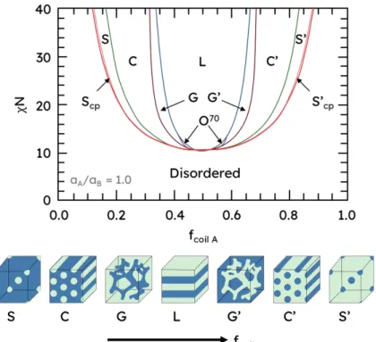
Figure 1-1. Canonical AB diblock copolymer phase diagram derived from self-consistent mean

field theory (SCFT) calculations.35 Phase abbreviations are as follows: S, S’: spheres, body-center cubic (BCC) spheres; Scp: close-packed spheres; C, C’: hexagonally packed cylinders; G,

G’: gyroid; O70_{: orthorhombic. The (’) indicates an inverse phase. The ratio a}

A:aB indicates the

ratio of statistical segment lengths. ... 31

Figure 1-2. Experimental phase diagram for solution-state mCherry-b-PNIPAM bioconjugates

(shown schematically in inset) at 25 °C, adapted from Thomas et al.49 ... 33

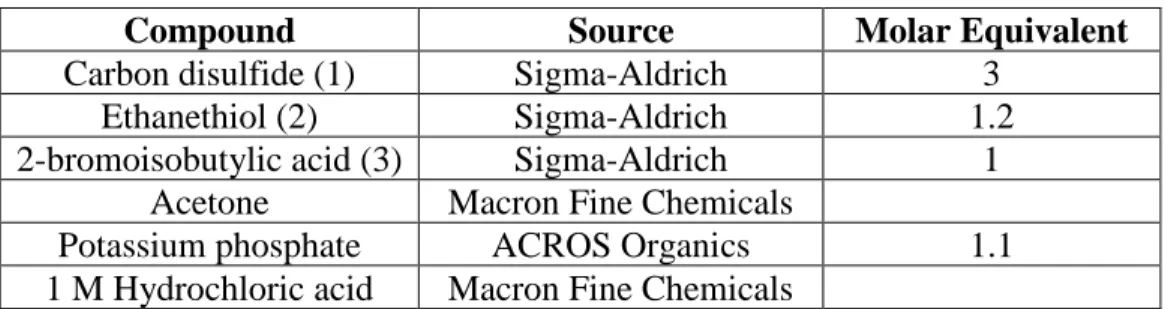
Figure 2-1. Synthesis of 2-(ethylsulfanylthiocarbonylsulfanyl)-2-methylpropionic acid (EMP)

from carbon disulfide, ethanethiol, and 2-bromoisobutylic acid. Molar ratios of each compound can be found in Table 2-1. ... 41

Figure 2-2. Chromatograph for EMP purification taken on a Biotage Isolera One Flash

Chromatography system. The solvent is 2:1 hexane:ethyl acetate. ... 42

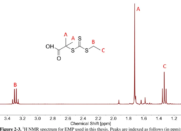
Figure 2-3. 1_{H NMR spectrum for EMP used in this thesis. Peaks are indexed as follows (in}

ppm): δA = 1.72, δB = 3.29, and δC = 1.33. The peaks were referenced to the solvent peak at 7.26

ppm (CDCl3). There are no additional peaks above the range shown here, besides the solvent

peak at CDCl3. ... 43 Figure 2-4. Synthesis of poly(N-isopropylacrylamide) (PNIPAM) by RAFT polymerization of

monomer NIPAM using EMP as a chain transfer agent and AIBN as the initiator. ... 43

Figure 2-5. (a) Airfree Schlenk flask (Chemglass part no. AF-0520-27) and accessories. The

copper wire is used to help seal the vessel, as shown in (b) an example of a sealed vessel with oval stir bar. For optimal stirring, use the oval stir bar in the reaction vessel and a paperclip to stir the oil bath. ... 45

Figure 2-6. Refractive index GPC trace for purified PNIPAM with Mn = 28,050 Da and Đ =

1.03... 45

Figure 2-7. 1H NMR spectrum for PNIPAM used in this thesis. Peaks are indexed as follows (in ppm): δA = 1.13, δB = 3.99, δC = 6.22, δD = 2.08, and δE = 1.33. The peaks were referenced to the

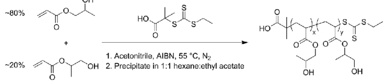
solvent peak at 7.26 ppm (CDCl3). There are no additional peaks above the range shown here. 46 Figure 2-8. Synthesis of poly(hydroxypropyl acrylate) (PHPA) by RAFT polymerization of

monomer HPA (95% mixture of monomers) using EMP as a chain transfer agent and AIBN as the initiator. ... 46

Figure 2-9. Refractive index GPC trace for purified PHPA with Mn = 27,960 Da and Đ = 1.07.

... 48

Figure 2-10. 1_{H NMR spectrum for PHPA used in this thesis. Peaks are indexed as follows (in}

ppm): δA,A’ = 1.19; δB = 4.00; δB’ = 3.62, 3.64; δC,C’ = 3.73; δD,D’ = 2.39; δE,E’ = 1.53, 1.71, 1.85,

1.97; δF = 4.00, and δF’ = 4.98. The peaks were referenced to the solvent peak at 7.26 ppm

(CDCl3, not shown). There are no additional peaks above the range shown here, besides the

solvent peak at CDCl3. To approximate the fraction of each monomer, the following ratio was

used: 𝐹′𝐷, 𝐷′ = 𝑦𝑥 + 𝑦 = 13.63 = 0.275. ... 48

Figure 2-11. Synthesis of poly(3-[N-(2-methacroyloyethyl)-N,N-dimethylammonio]propane

sulfonate) (PDMAPS) by RAFT polymerization of monomer DMAPS using CPP as a chain transfer agent and VA-044 as the initiator. ... 49

Figure 2-12. GPC traces for purified PDMAPS with Mn = 32,500 Da and Đ = 1.18. LS signifies

(15)

15

Figure 2-13. 1_{H NMR spectrum for PDMAPS used in this thesis. Peaks are indexed as follows}

(in ppm): δA = 2.28, δB = 3.60, δC = 3.23, δD = 2.98, δE = 3.81, δF = 4.50, δG = 1.99, and δH =

1.00-1.14. The peaks were referenced to the solvent peak at 4.79 (D2O). The quartet at 3.97 ppm

can be indexed to residual trifluoroethanol. ... 51

Figure 2-14. Screenshot of Astra 6.1 showing an example GPC trace for PNIPAM. The baseline

was corrected for the signal from each detector in the table. The range over which the baseline is calculated can be adjusted by dragging the width of the black selection window. ... 52

Figure 2-15. (a) DPLS sample holder pieces from left to right: brass outer cell, o-ring, quartz

window, Teflon spacer, quartz window, o-ring, and brass fastener. (b) DPLS sample holder after assembly. ... 54

Figure 2-16. Schematic of coarse-grained model and physical protein and polymer on which it is

based. (a) mCherry structure and size (b) Chemical structure of poly(N-isopropylacrylamide) (PNIPAM) (c) Structure of mCherry-b-PNIPAM bioconjugate (d) Coarse-grained dumbbell model of bioconjugate consisting of a hard sphere (green, representing protein) and a soft sphere (blue, representing polymer) with relevant length scales noted (e) Bioconjugates with coil fractions (fcoil) probed by simulations with equivalent polymer sizes (polymer radius of gyration,

Rg2) ... 61

Figure 2-17. A general overview of a molecular dynamics (MD) simulation ... 62 Figure 3-1. Order-disorder transition concentration, or CODT, for bioconjugates of mCherry and PNIPAM, POEGA, and PDMAPS, the three polymers studied here at different coil fractions (φcoil). The CODT is defined as the minimum concentration in solution at which order is observed. A lower CODT corresponds to a higher propensity for order. For this study, the equal volume ratios of protein to polymer correspond to a coil fraction of 0.5. ... 88

Figure 3-2. Chemical structures and molar masses of (a) PNIPAM, (b) POEGA, and (c)

PDMAPS. Cartoon of (d) mCherry, a beta-barrel protein. Dimensions for each polymer are reported as radius of gyration or fully extended end-to-end distance (contour length). Protein radius of gyration, as well as beta barrel dimensions are reported in (d). ... 90

Figure 3-3. Variations of SLD as a function of solvent composition corrected for exchangeable

protons in mCherry and hydration of the polymers ... 94

Figure 3-4. Absolute scattering intensities at various solvent fractions of D2O for mCherry

blends with (a) PNIPAM, (b) POEGA, and (c) PDMAPS. Experimentally obtained data is represented as open red squares, and reconstructed data from the decomposed partial scattering functions is represented as solid black lines. Data is multiplicatively offset by factors of 1, 10, 100, and 1000 for clarity. These curves do not reflect background and incoherent scattering correction, which was performed prior to decomposition and added back for the purpose of reconstruction. All percentages are % (v/v). ... 95

Figure 3-5. Decomposed partial structure factors for (a) PNIPAM, (b) POEGA, and (c)

PDMAPS. Self-correlation terms for the protein and polymer are represented by open circles and squares, respectively. Cross-correlation terms between the protein and polymer are represented by open diamonds. Smoothed data are represented by solid lines. ... 96

Figure 3-6. Single molecule and intermolecular components of the non-dimensionalized

protein-protein structure factor S11* in the presence of (a) PNIPAM, (b) POEGA, and (c) PDMAPS. The single molecule component P1cyl is the cylinder form factor for mCherry. The intermolecular component P11I is scaled by the volume fraction of mCherry. ... 97

Figure 3-7. Single chain and interchain components of the non-dimensionalized

(16)

16

molecule component P2Debye is the Debye form factor for Gaussian chains. The intermolecular component P22I is scaled by the volume fraction of polymer ... 98

Figure 3-8. Dimensionless concentration correlation function Γij* between components i and j

for (a) PNIPAM/mCherry, (b) POEGA/mCherry blend, and (c) PDMAPS/mCherry. ... 101

Figure 3-9. Interactions between mCherry and (a) PNIPAM (b) POEGA, and (c) PDMAPS.

PNIPAM drives a depletion interaction between mCherry molecules. POEGA experiences attractive interactions with mCherry molecules, leading to polymer adsorption close to the protein surface. PDMAPS also experiences attractive interactions with mCherry molecules but they are weaker than that of POEGA and driven by electrostatics. PDMAPS also induces

depletion interactions between mCherry molecules. The electrostatic surface potential (± 5 kT/ec,

with red and blue representing negative and positive values, respectively) at the

solvent-accessible surface of mCherry is rendered from the Adaptive Poisson-Boltzmann Solver (APBS) plugin of PyMOL.54-57 For mCherry and PDMAPS, red represents negative charge and blue represents positive charge. Nonionic polymers are depicted as black. ... 102

Figure 3-10. Variation in dimensionless correlation function Γij* with respect to hydration water

for (a) PNIPAM/PNIPAM interactions and (b) PNIPAM/mCherry interactions demonstrating that hydration number tunes the strength but not nature of interactions... 106

Figure 4-1. SDS-PAGE gel for TEV-CG-eGFP and conjugates. The lanes are as follows (from

left): (1) Ladder (2) TEV-CG-eGFP (3) LPAA-eGFP (4) DPAA-eGFP (5) LDPAA-eGFP ... 120

Figure 4-2. CD spectra for (a) poly(amino acids) alone and (b) bioconjugates and eGFP. All raw

CD signals (measured in mdeg) were converted into molar ellipticity. Error bars are ± 1σ. ... 124

Figure 4-3. CD spectra for variants of (a) LPAA, (b) DPAA, (c) LDPAA, and (d) eGFP. For all

four figures, the eGFP spectrum measured from a solution of only eGFP is shown in closed black circles. For figures (a) – (c), the CD spectra for the bioconjugates (XPAA-eGFP) are shown in closed colored circles (red for LPAA, blue for DPAA, and green in LDPAA). The CD spectra for the PAA while in the bioconjugate are shown in open circles; this was calculated by subtracting out the eGFP signal. The CD spectra for the PAA only (not in a bioconjugate) are shown in open squares. For figure (d), the CD spectra for eGFP in each type of conjugate after subtracting out the PAA signal is shown in colored circles (red for LPAA, blue for DPAA, and green for

LDPAA). ... 126

Figure 4-4. Phase diagrams for (a) eGFP, (b) DPAA-eGFP, and (c) 1:1 blend of

LPAA-eGFP and DPAA-LPAA-eGFP (L:D1:1-LPAA-eGFP). None of the samples showed significant birefringence, with all power fractions below 0.15. Birefringence curves for each sample can be found in the SI. ... 128

Figure 4-5. SAXS intensity curves for LPAA-eGFP at (a) 10 °C and (b) 50 °C for selected

concentrations (wt%). The lamellar peaks (q*, 2q*, 3q*, 4q*) are labeled for both lamellar phases (low concentration 1 and high concentration 2). SAXS patterns are offset for clarity. 45 wt% forms both lamellar phases. ... 130

Figure 4-6. SAXS intensity curves for all bioconjugates at 50 wt% for (a) 10 °C and (b) 50 °C.

The lamellar peaks (q*, 2q*) are labeled for the LPAA-eGFP curve. SAXS patterns are offset for clarity. All peaks observed in LPAA-eGFP, DPAA-eGFP, and L:D1:1-eGFP correspond to lamellae. The peaks in (b) correspond to aggregation at high temperature in LDPAA-eGFP samples. ... 130

Figure 4-7. (a) Dimensions of a bioconjugate. The eGFP block is a β-barrel modeled as a

cylinder. It has two hydration shells. The PAA block is an α-helix with (EG)3 side chains (shown

(17)

17

DPAA-eGFP. The domain spacing was averaged over all the temperatures over which a specific sample formed the same phase, since it is independent of temperature. Error bars represent ± 1σ. For all three types of bioconjugates, the domain spacing has a non-monotonic trend with the concentration. The closed circles represent domain spacing calculated from the main SAXS peak. The open square is the domain spacing calculated for the second set of peaks for LPAA-eGFP at 45 wt%, which exhibited two lamellar phases. The dashed lines (- -) represent the theoretical domain spacing if the bioconjugates arranged into bilayers or interdigitated layers, as shown in the inset schematics. The L:D1:1-eGFP blend (Figure B-16) was similar to both the LPAA and DPAA, with two lamellar phases at 45 wt%. ... 132

Figure 4-8. Size distribution histograms measured from DLS (represented as %intensity as a

function of diameter) for (a) LPAA-eGFP, (b) DPAA-eGFP, (c) L:D1:1-eGFP, and (d) LDPAA-eGFP at 1 mg/mL in water. Each curve represents a replicate. ... 135

Figure 4-9. UV-Vis absorbance curves for LPAA-eGFP (red), DPAA-eGFP (blue),

L:D1:1-eGFP (purple), and LDPAA-L:D1:1-eGFP (green) at 0.5 mg/mL in water ... 137

Figure 5-1. Process flow diagram for calculating hydration number (nH) from (a) dilute and (b) semidilute and concentrated solutions of polymers. For the generalized fit used in semidilute and concentrated solutions, there are two pathways to obtaining the hydration number: (i) fitting Δρ(f) and solving for nH through Equation 5.4.1 or (ii) fitting for nH directly. In both cases, Δρ(f) is needed for the contrast matching procedure (Equation 5.4.6) to obtain the volume vp. ... 150

Figure 5-2. Debye form factor fits (green lines) to SANS intensity data (dark blue squares) taken

for (a) PNIPAM, (b) PHPA, and (c) PDMAPS in 100% D2O at 13.75 mg/mL. The fits were done

using D-FF-SLD. The data shown in black squares represent 100 bootstrapped replicas of the original experiment. Error bars on inset parameters represent ±1σ from 100 replicas. ... 152

Figure 5-3. Scaled SANS intensity curves taken for dilute solution PNIPAM (13.75 mg/mL) fit

using the methods described in Table 5-2: (a) D-FF-SLD, (b) CV-MF-SLD, (c) CV-FF-SLD, (d) CV-FF-nH, (e) CV-SF-SLD and (f) CV-SF-nH. The subplot for the D-FF-SLD method includes

all 100 replicas of the SANS intensity curve taken in 100% D2O (dark blue squares), with the

light orange line representing the Debye fit. For clarity, methods (b) – (f) include only replica 1 (the original experiment, squares), with solid lines representing the fits. Error bars are standard deviation from the instrument. ... 157

Figure 5-4. Bar charts comparing the hydration number obtained through different fitting

methods for (a) PNIPAM, (b) PHPA, and (c) PDMAPS in dilute solution (13.75 mg/mL). The light blue bars represent hydration numbers averaged across high D2O blends. For PDMAPS, the

nH direct fits yield a hydration number of 0 with very small error bars. Error bars represent standard error of the mean from 100 replicas. ... 158

Figure 5-5. Bar charts comparing the hydration number obtained through different fitting

methods in the semi-dilute and concentrated regimes. Top row: (a) PNIPAM, (b) PHPA, and (c) PDMAPS in semidilute solution (50 mg/mL). Bottom row: (d) PNIPAM, (e) PHPA, and (f) PDMAPS in concentrated solution (250 mg/mL). Hydration numbers for 300 mg/mL solutions can be found in Figure C-52. The hydration numbers obtained from SLD (dark and light blue bars) are from the CV-SANS approach (i), and directly fit hydration numbers are from approach (ii). The light blue bars represent hydration numbers averaged across high D2O blends. Error bars

represent standard error of the mean from 100 replicas. ... 162

Figure 5-6. (a) Hydration number and (b) scaled hydration number as a function of polymer

concentration in solution. The colors are chosen to match those in Figure 5-4 and Figure 5-5, where green represents nH-based fitting methods (here, CV-FF-nH and CV-SF-nH), and blue

(18)

18

represents SLD-based methods (here, CV-MF-SLD). Open symbols are hydration numbers obtained from CV-FF-nH, and closed symbols are hydration numbers obtained from the

CV-MF-SLD or CV-SF-nH fits. Error bars (standard error of the mean over 100 replicas) are smaller than

the symbols. ... 166

Figure 6-1. Schematic of coarse-grained HS dumbbell model and physical protein and polymer

on which it is based. (a) mCherry structure and size (b) Chemical structure of

poly(N-isopropylacrylamide) (PNIPAM) (c) Structure of mCherry-b-PNIPAM bioconjugate (d) Coarse-grained HS dumbbell model of bioconjugate consisting of a hard sphere (green, representing protein) and a soft sphere (blue, representing polymer) with relevant length scales noted (e) Bioconjugates with selected coil fractions probed by simulations with equivalent polymer sizes ... 182

Figure 6-2. Intermolecular potentials for the (a) hard–hard (1–1) and soft–soft (2–2) interactions

at different coil fractions, (b) hard–hard and hard–soft (1–2) interactions at different values of

U12(0), and (c) hard–hard and hard–soft (1–2) interactions at different coil fractions. ... 184

Figure 6-3. Phase diagrams from MD simulations obtained using U12(0) of (a) 20kBT, (b) 50kBT, and (c) 100kBT. The experimental phase diagram for mCherry-b-PNIPAM bioconjugates

obtained from SAXS experiments8, 9 is shown in panel (d). The simulation snapshots are taken from the U12(0) = 20kBT phase diagram. ... 190

Figure 6-4. The onset of hard sphere packing as a function of concentration in a dumbbell with a

coil fraction of 0.67 and U12 (0) = 20kBT. Lamellar slices were taken for (a) (i) 20% and (ii) 70%, showing hexagonally packed hard spheres in (ii), with the 2D structure factor shown in (b). (c) Radial distribution function of only hard spheres for four concentrations, for which simulation snapshots are shown in insets for (i) 10%, (ii) 20%, (iii) 70%, and (iv) 100%. ... 196

Figure A-1. SDS-PAGE of FPLC purified mCherry. Lanes contain the following: 1-12) elutions

at 24 mL to 73.5 mL in increments of 4.5 mL. Lane 13 is the column wash with 2M NaCl after elution. Column volume was 10 mL. ... 211

Figure A-2. Gel permeation chromatography (GPC) traces for PNIPAM (Mn = 26.3 kDa, Đ = 1.08), POEGA (Mn = 26.4 kDa, Đ = 1.13), and PDMAPS (Mn = 26.7 kDa, Đ = 1.10). ... 212

Figure A-3. Debye form factor fits for (a) PNIPAM, (b) POEGA, and (c) PDMAPS. Open

squares are experimental SANS absolute intensities with incoherent background subtracted. The red line is the Debye form factor fit calculated using the inset radii of gyration and polymer SLD. Uncertainties are 1𝜎. ... 214

Figure A-4. Variation in scattering length density (SLD) with hydration number (nH) and solvent volume fraction of D2O for (a) PNIPAM, (b) POEGA, and (c) PDMAPS. ... 215 Figure A-5. Absolute SANS intensity curves for (a) PNIPAM, (b) POEGA, and (c) PDMAPS

showing the estimated background and incoherent scattering component that was subtracted prior to partial structure factor decomposition. Data for Q < 1 nm-1 have been truncated for clarity. The gray box illustrates the range over which the intensity was averaged. ... 217

Figure A-6. Linearized Guinier-like fits for scattering intensities of blends of mCherry and (a)

PNIPAM, (b) POEGA, and (c) PDMAPS. Fitting parameters for Equation A.6.9 are displayed next to the corresponding line of fit. Dashed lines indicate 95% confidence intervals for each fit. ... 218

Figure A-7. Results of Guinier-like fit (Equation A.6.9) used to extrapolate to Q = 0 nm-1 for absolute scattering intensities after background subtraction of blends of mCherry and (a)

(19)

19

Figure A-8. Dimensionless concentration correlation function Γij* between components i and j

for (a, d) PNIPAM/mCherry, (b, e) POEGA/mCherry blend, and (c, f) PDMAPS/mCherry. The set of figures shown in (a – c) were derived from the experimental data with only high Q extrapolation. The set of figures shown in (d – f) were derived from experimental data

extrapolated on both the low and high Q ends. ... 219

Figure A-9. Single molecule and intermolecular components of the non-dimensionalized

protein-protein structure factor S11* plotted on a log-log scale in the presence of (a) PNIPAM, (b) POEGA, and (c) PDMAPS. The single molecule component P1cyl is the cylinder form factor for mCherry. ... 221

protein-protein structure factor S11* plotted on a log-linear scale in the presence of (a) PNIPAM, (b) POEGA, and (c) PDMAPS. The single molecule component P1cyl is the cylinder form factor for mCherry. ... 221

polymer-polymer structure factor S22* plotted on a log-log scale for (a) PNIPAM, (b) POEGA, and (c) PDMAPS. The single molecule component P2Debye is the Debye form factor for Gaussian chains. ... 222

polymer-polymer structure factor S22* plotted on a log-linear scale for (a) PNIPAM, (b) POEGA, and (c) PDMAPS. The single molecule component P2Debye is the Debye form factor for Gaussian chains. ... 222

Figure A-13. Variation in dimensionless partial structure factor Sij* with respect to hydration water for (a) PNIPAM/PNIPAM interactions, (b) PNIPAM/mCherry interactions, (c)

POEGA/POEGA interactions, (d) POEGA/mCherry interactions, (e) PDMAPS/PDMAPS interactions, and (f) PDMAPS/mCherry interactions demonstrating that hydration number tunes the strength but not nature of interactions. ... 223

Figure A-14. Variation in dimensionless concentration correlation function Γij* with respect to

hydration water for (a) POEGA/POEGA interactions, (b) POEGA/mCherry interactions, (c) PDMAPS/PDMAPS interactions, and (d) PDMAPS/mCherry interactions demonstrating that hydration number tunes the strength but not nature of interactions... 224

Figure B-1. Normalized differential refractive index (dRI) signal as a function of retention time

as measured from GPC for each PAA. ... 225

Figure B-2. Proton NMR spectrum of P(EG)3-L-Glu88 PAA (LPAA) with proton groups labeled

on the inset molecule. Peak areas are shown underneath the spectrum and peak chemical shifts are shown next to each peak with the proton group. ... 226

Figure B-3. Proton NMR spectrum of P(EG)3-D-Glu97 PAA (DPAA) with proton groups labeled

on the inset molecule. Peak areas are shown underneath the spectrum and peak chemical shifts are shown next to each peak with the proton group. ... 226

Figure B-4. Proton NMR spectrum of P(EG)3-L/D-Glu100 PAA (LDPAA) with proton groups

labeled on the inset molecule. Peak areas are shown underneath the spectrum and peak chemical shifts are shown next to each peak with the proton group. ... 227

Figure B-5. Mass spectra of TEV-CG-eGFP and CG-eGFP. ... 227 Figure B-6. Cloud point temperature (Tcp) of all PAAs as a function of concentration in aqueous solution. For all PAAs, Tcp was too high to measure during SAXS because eGFP is expected to denature by 50 °C. The right axis is labeled with the estimated cloud point temperature at high concentration (300 mg/mL). ... 228

(20)

20

Figure B-7. SAXS intensity curves for LPAA-eGFP at (a) 10 °C, (b) 15 °C, (c) 20 °C, (d) 25 °C,

(e) 30 °C, (f) 35 °C, (g) 40 °C, (h) 45 °C, and (i) 50 °C. For each plot, from bottom to top, the concentration varies from 20 to 60 wt% in 5 wt% increments. SAXS curves are offset for clarity. ... 229

Figure B-8. SAXS intensity curves for DPAA-eGFP at (a) 10 °C, (b) 15 °C, (c) 20 °C, (d) 25 °C,

(e) 30 °C, (f) 35 °C, (g) 40 °C, (h) 45 °C, and (i) 50 °C. For each plot, from bottom to top, the concentration varies from 20 to 60 wt% in 5 wt% increments. SAXS curves are offset for clarity. ... 230

Figure B-9. SAXS intensity curves for L:D1:1-eGFP at (a) 10 °C, (b) 15 °C, (c) 20 °C, (d)

25 °C, (e) 30 °C, (f) 35 °C, (g) 40 °C, (h) 45 °C, and (i) 50 °C. For each plot, from bottom to top, the concentration varies from 20 to 60 wt% in 5 wt% increments. SAXS curves are offset for clarity. ... 231

Figure B-10. SAXS intensity curves for LDPAA-eGFP at (a) 10 °C, (b) 15 °C, (c) 20 °C, (d)

25 °C, (e) 30 °C, (f) 35 °C, (g) 40 °C, (h) 45 °C, and (i) 50 °C. For each plot, from bottom to top, the concentration varies from 20 to 60 wt% in 5 wt% increments. SAXS curves are offset for clarity. ... 232

Figure B-11. LPAA-eGFP birefringence (power fraction) and transmission curves as a function

of temperature as measured by depolarized light scattering (DPLS). Heating ramps are depicted in red, and cooling ramps are depicted in blue. Each double panel corresponds to a different wt%: (a) 25%, (b) 30%, (c) 35%, (d) 40%, (e) 45%, (f) 50%, (g) 55%, (h) 60%. There is no plot for 20% because this sample was too liquid-like to remain in the sample holder. Based on the behavior of the more dilute samples, 20% is not expected to exhibit any birefringence. ... 233

Figure B-12. DPAA-eGFP birefringence (power fraction) and transmission curves as a function

of temperature as measured by depolarized light scattering (DPLS). Heating ramps are depicted in red, and cooling ramps are depicted in blue. Each double panel corresponds to a different wt%: (a) 20%, (b) 25%, (c) 30%, (d) 35%, (e) 40%, (f) 45%, (g) 50%, (h) 55%, (i) 60%. ... 234

Figure B-13. L:D1:1-eGFP birefringence (power fraction) and transmission curves as a function

of temperature as measured by depolarized light scattering (DPLS). Heating ramps are depicted in red, and cooling ramps are depicted in blue. Each double panel corresponds to a different wt%: (a) 20%, (b) 25%, (c) 30%, (d) 35%, (e) 40%, (f) 45%, (g) 50%, (h) 55%, (i) 60%. ... 235

Figure B-14. LDPAA-eGFP birefringence (power fraction) and transmission curves as a

function of temperature as measured by depolarized light scattering (DPLS). Heating ramps are depicted in red, and cooling ramps are depicted in blue. Each double panel corresponds to a different wt%: (a) 20%, (b) 25%, (c) 30%, (d) 35%, (e) 40%, (f) 45%, (g) 50%. There are no data for 55 and 60 wt% because these were too turbid to measure. ... 236

Figure B-15. Domain spacing as a function of concentration at different temperatures for (a)

LPAA-eGFP, (b) DPAA-eGFP, and (c) L:D1:1-eGFP. There is a non-monotonic dependence of domain spacing on concentration due to the presence of two lamellar phases but no significant dependence on temperature. The open square is the domain spacing calculated for the second set of peaks for 45 wt%, which exhibited two lamellar phases in samples containing LPAA-eGFP. ... 237

Figure B-16. Domain spacing as a function of concentration averaged over all temperatures for

L:D1:1-eGFP. There is a non-monotonic dependence of domain spacing on concentration. The closed circles represent domain spacing calculated from the main SAXS peak. The open square is the domain spacing calculated for the second set of peaks for 45 wt.%, which exhibited two lamellar phases. ... 237

(21)

21

Figure B-17. CD spectra for 1:1 blend of LPAA-eGFP and DPAA-eGFP before and after

lyophilization at (a) 10 °C, (b) 25 °C, and (c) 50 °C. ... 238

Figure B-18. SAXS subtracted intensity curves for LDPAA-eGFP with a fit to the hard sphere

structure factor (Equations B.10.15, B.10.16, and B.10.18) for (a) 45 wt%, 45 °C, (b) 45 wt%, 50 °C, (c) 50 wt%, 35 °C, (d) 50 wt%, 40 °C, (e) 50 wt%, 45 °C, and (f) 50 wt%, 50 °C... 241

Figure C-1. Relative refractive index (RI) GPC trace for purified PNIPAM with Mn = 28,050 Da

and Đ = 1.03. ... 242

Figure C-2. Relative refractive index (RI) GPC trace for purified PHPA with Mn = 27,960 Da

and Đ = 1.07. ... 242

Figure C-3. Relative refractive index (RI) GPC trace for purified PDMAPS with Mn = 32,500

Da and Đ = 1.18. ... 243

Figure C-4. 1H NMR spectrum for PNIPAM. Peaks are indexed as follows (in ppm): δA = 1.13,

δB = 3.99, δC = 6.22, δD = 2.08, and δE = 1.33. The peaks were referenced to the solvent peak at

7.26 ppm (CDCl3). There are no additional peaks above the range shown here. ... 243 Figure C-5. 1_{H NMR spectrum for PHPA. Peaks are indexed as follows (in ppm): δ}_A,A’_{= 1.19;}

δB = 4.00; δB’ = 3.62, 3.64; δC,C’ = 3.73; δD,D’ = 2.39; δE,E’ = 1.53, 1.71, 1.85, 1.97; δF = 4.00, and

δF’ = 4.98. The peaks were referenced to the solvent peak at 7.26 ppm (CDCl3, not shown). There

are no additional peaks above the range shown here, besides the solvent peak at CDCl3. To

approximate the fraction of each monomer, the following ratio was used: 𝐹′𝐷, 𝐷′ = 𝑦𝑥 + 𝑦 = 13.63 = 0.275. ... 244

Figure C-6. 1H NMR spectrum for PDMAPS used in this thesis. Peaks are indexed as follows (in ppm): δA = 2.28, δB = 3.60, δC = 3.23, δD = 2.98, δE = 3.81, δF = 4.50, δG = 1.99, and δH =

1.00-1.14. The peaks were referenced to the solvent peak at 4.79 (D2O). The quartet at 3.97 ppm

can be indexed to residual trifluoroethanol. ... 244

Figure C-7. Cloud point curves for (a) PNIPAM, (b) PHPA, and (c) PDMAPS. PNIPAM and

PHPA are LCST polymers, and PDMAPS is an UCST polymer. ... 246

Figure C-8. SANS fitting through CV-MF-SLD for (a) PNIPAM, (b) PHPA, and (c) PDMAPS

at 13.75 mg/mL ... 246

at 50 mg/mL ... 247

at 250 mg/mL ... 247

at 300 mg/mL ... 247

Figure C-12. SANS fitting through CV-FF-SLD for (a) PNIPAM, (b) PHPA, and (c) PDMAPS

at 13.75 mg/mL ... 248

Figure C-13. SANS fitting through CV-FF-nH for (a) PNIPAM, (b) PHPA, and (c) PDMAPS at

13.75 mg/mL ... 248

Figure C-14. SANS fitting through CV-SF-SLD for (a) PNIPAM, (b) PHPA, and (c) PDMAPS

at 13.75 mg/mL ... 248

at 50 mg/mL ... 249

at 250 mg/mL. PNIPAM does not have a Zimm structure factor at high concentration. ... 249

(22)

22

Figure C-18. SANS fitting through CV-SF-nH for (a) PNIPAM, (b) PHPA, and (c) PDMAPS at

13.75 mg/mL ... 250

50 mg/mL ... 250

250 mg/mL. PNIPAM does not have a Zimm structure factor at high concentration. ... 250

300 mg/mL. PNIPAM does not have a Zimm structure factor at high concentration. ... 251

Figure C-22. SLD of polymer determined through CV-MF-SLD for (a) PNIPAM, (b) PHPA,

and (c) PDMAPS at 13.75 mg/mL ... 251

and (c) PDMAPS at 50 mg/mL ... 252

Figure C-26. SLD of polymer determined through CV-FF-SLD for (a) PNIPAM, (b) PHPA, and

(c) PDMAPS at 13.75 mg/mL ... 253

Figure C-27. SLD of polymer determined through CV-FF-nH for (a) PNIPAM, (b) PHPA, and

(c) PDMAPS at 13.75 mg/mL ... 253

Figure C-28. SLD of polymer determined through CV-SF-SLD for (a) PNIPAM, (b) PHPA, and

(c) PDMAPS at 13.75 mg/mL ... 254

(c) PDMAPS at 50 mg/mL ... 254

Figure C-32. SLD of polymer determined through CV-SF-nH for (a) PNIPAM, (b) PHPA, and

(c) PDMAPS at 13.75 mg/mL ... 255

Figure C-36. Form factor of PNIPAM in 13.75 mg/mL solution determined through (a)

D-FF-SLD, (b) CV-MF-D-FF-SLD, (c) CV-FF-D-FF-SLD, (d) CV-FF-nH, (e) CV-SF-SLD and (f) CV-SF-nH. In

this case, both P(q) and G(q) refer to the form factor. ... 257

Figure C-37. Form factor of PHPA in 13.75 mg/mL solution determined through (a) D-FF-SLD,

(b) CV-MF-SLD, (c) CV-FF-SLD, (d) CV-FF-nH, (e) CV-SF-SLD and (f) CV-SF-nH. In this

case, both P(q) and G(q) refer to the form factor. ... 258

Figure C-38. Form factor of PDMAPS in 13.75 mg/mL solution determined through (a)

D-FF-SLD, (b) CV-MF-D-FF-SLD, (c) CV-FF-D-FF-SLD, (d) CV-FF-nH, (e) CV-SF-SLD and (f) CV-SF-nH. .. 259 Figure C-39. Structure factor of PNIPAM in 50 mg/mL solution determined through (a)

(23)

23

Figure C-40. Structure factor of PHPA in 50 mg/mL solution determined through (a)

CV-MF-SLD, (b) CV-SF-CV-MF-SLD, and (c) CV-SF-nH ... 260 Figure C-41. Structure factor of PDMAPS in 50 mg/mL solution determined through (a)

CV-MF-SLD, (b) CV-SF-SLD, and (c) CV-SF-nH ... 260 Figure C-42. Structure factor of PNIPAM in 250 mg/mL solution determined through (a)

CV-MF-SLD, (b) CV-SF-SLD, and (c) CV-SF-nH ... 260 Figure C-43. Structure factor of PHPA in 250 mg/mL solution determined through (a)

CV-MF-SLD, (b) CV-SF-SLD, and (c) CV-SF-nH ... 261 Figure C-45. Structure factor of PNIPAM in 300 mg/mL solution determined through (a)

CV-MF-SLD, (b) CV-SF-SLD, and (c) CV-SF-nH ... 261 Figure C-46. Structure factor of PHPA in 300 mg/mL solution determined through (a)

CV-MF-SLD, (b) CV-SF-SLD, and (c) CV-SF-nH ... 262 Figure C-48. Box-and-whisker plots for hydration number obtained through different fitting

methods for (a) PNIPAM, (b) PHPA, and (c) PDMAPS in dilute solution (13.75 mg/mL). ... 263

Figure C-49. Box-and-whisker plots for hydration number obtained through different fitting

methods for (a) PNIPAM, (b) PHPA, and (c) PDMAPS in semidilute solution (50 mg/mL). CV-SF-SLD did not converge for PHPA. ... 263

methods for (a) PNIPAM, (b) PHPA, and (c) PDMAPS in concentrated solution (250 mg/mL). PNIPAM does not take on a Zimm structure factor in concentrated solution. ... 264

methods for (a) PNIPAM, (b) PHPA, and (c) PDMAPS in concentrated solution (300 mg/mL). PNIPAM does not take on a Zimm structure factor in concentrated solution. ... 264

Figure C-52. Bar charts comparing the hydration number obtained through different fitting

methods in the concentrated regime (300 mg/mL). (a) PNIPAM, (b) PHPA, and (c) PDMAPS The hydration numbers obtained from SLD (dark and light blue bars) are from the CV-SANS approach (i), and directly fit hydration numbers are from approach (ii). The light blue bars represent hydration numbers averaged across high D2O blends. Error bars represent standard

error of the mean from 100 replicas. ... 265

Figure C-53. Fits to Equation C.10.1 for PNIPAM in (a) 250 and (b) 300 mg/mL solution (100%

D2O). Error bars (standard deviation from the instrument) are smaller than the size of the data

point. ... 267

Figure D-1. Structure factors for simulations run with U12(0) = 20kBT and a coil fraction of 0.67 for concentrations of (a) 10%, (b) 20%, (c) 70%, and (d) 100%. ... 274

Figure D-2. Phase diagram for U12(0) = 9 kBT ... 274

Figure D-3. Phase diagram for U12(0) = 200 kBT ... 275

Figure G-1. (a) Full protein sequence for ELP-mCherry, including His-tag. The asterisk (*)

designates the stop codon. Relevant protein regions are highlighted. (b) Plasmid map for

pET28a(+)-ELP-mCherry. KanR indicates kanamycin resistance. ... 331

Figure G-2. Fermenter stirring speed controller. The optimized stirring speed is set by having

(24)

24

Figure G-3. Visual results of ammonium sulfate test precipitation. (a) The resulting suspensions

after adding 3 M ammonium sulfate to the final labeled concentrations. (b) The resulting

separation between supernatant and pellet after the first “hot spin” step (centrifugation at 4 °C for 30 min at 13,100 x g). ... 333

Figure G-4. Overview of inverse thermal cycling (ITC) process used to purify ELP-mCherry

and its deuterated analogue. The cold and hot spins are labeled; note that the hot spin is done using salt instead of temperature. The salt used here is ammonium sulfate. ... 334

Figure G-5. SDS-PAGE gel illustrating the typical ELP-mCherry purities attained after inverse

transition cycling purification (ITC). The lanes are as follows: (1) clarified lysate, (2) supernatant after first hot spin, (3) pellet after first hot spin, (4) supernatant after second hot spin, (5)

supernatant after first cold spin,* (6) pellet after first cold spin,* (7) supernatant after second hot spin,* (8) pellet after second hot spin, (9) pellet after second hot spin,* (10) pellet after second hot spin, * (11) pellet after second cold spin, (12) supernatant after second cold spin, (13) pellet after second cold spin*, (14) supernatant after second cold spin.* The asterisk (*) indicates a step that has been repeated due to residual ELP-mCherry in the wrong fractions (i.e. pure protein should not be in a hot spin supernatant or a cold spin pellet). The presence of residual ELP-mCherry in the wrong fraction is due to an excess of protein from overexpression. ... 335

Figure G-6. (a) Anion exchange FPLC chromatogram for ELP-mCherry showing the A280 trace

(cyan), the corresponding FPLC Buffer B concentration (green), and the fraction collection (each space between red tick marks is a separate fraction). (b) SDS-PAGE gels corresponding to selected FPLC fractions from the trace in (a). Pure protein was collected from fractions 5A10 – 5E5. ... 337

Figure G-7. SDS-PAGE gel showing the final purified ELP-mCherry. Each gel band is labeled.

There are two cleavage products due to the hydrolysis of an mCherry fragment during the

denaturation process of SDS-PAGE. ... 338

Figure G-8. Growth curves for test expressions using (a) condition 1: growth at 37 °C, followed

by expression at 20 °C (b) condition 2: growth at 30 °C, followed by expression at 20 °C, and (c) condition 3: growth and expression at 30 °C. Panel (a) shows a full growth curve, where time point 0 h is when the cells were induced. Panels (b) and (c) have been truncated to only show the growth after induction. ... 342

Figure G-9. Growth curve for full-scale expression of dELP-mCherry. Each color is a different

250 mL batch grown and expressed at the same conditions in the same refrigerated shaker. .... 342

Figure G-10. SDS-PAGE gel for ITC and FPLC of dELP-mCherry. Lanes 1 – 6 after the ladder

represent ITC fractions, and lanes 5 – 14 represent FPLC fraction well numbers. Lanes 1 – 6 are as follows: (1) supernatant after first hot spin, (2) pellet after first cold spin, (3) supernatant after first cold spin, (4) supernatant after second hot spin, (5) pellet after second cold spin, and (6) supernatant after second cold spin, which was dialyzed 3 times in Milli-Q water prior to running FPLC, shown in the subsequent lanes... 343

Figure G-11. Anion exchange FPLC chromatogram for dELP-mCherry showing the A280 trace

(cyan), the corresponding FPLC Buffer B concentration (green), and the fraction collection (each space between red tick marks is a separate fraction). Selected fractions were evaluated by SDS-PAGE gel shown in Figure G-10. The fractions collecting in 1A1, 1A2, 1B1, and 1B2 are protein impurities with an A280 signal. ... 344

Figure G-12. SDS-PAGE gel for dELP-mCherry for Ni-NTA chromatography. The lanes are as

follows. FT: flowthrough, W1: first wash, W2: second wash, E: eluted fraction. The final product is in the eluted fraction. ... 345

(25)

25

Figure G-13. MALDI-TOF mass spectra of dELP-mCherry in water (blue), dELP-mCherry in

D2O (red), and ELP-mCherry in water (black). The main peaks are labeled as (a) full length

singlet, (b) large fragment singlet, (c) full length doublet, and (d) large fragment doublet. The small fragment singlet is not expected to be within the range of m/z measured here. ... 346

Figure G-14. SDS-PAGE gel showing the purified ELP-mCherry (H) and its deuterated

analogue (D). The deuterated protein has two bands at ~ 80 kDa which can be attributed to populations of protein with different levels of deuteration and/or H/D exchange. ... 347

Figure G-15. (a) Circular dichroism (CD) spectra for dELP-mCherry and ELP-mCherry

showing that protein fold has not been affected significantly by deuteration. (b) UV-Vis spectra for dELP-mCherry and ELP-mCherry, showing that mCherry optical activity has not been affected significantly by deuteration. ... 347

Figure H-1. Schematic illustrating (a) amino acid sequences and components of P4 protein and

(b) hydrogel network structure... 351

Figure H-2. SDS-PAGE gel showing typical P4 purities for each fraction of ammonium sulfate

precipitation. S1: supernatant after first spin; P1: pellet after first spin; S2: supernatant after second spin; P2: pellet after second spin. ... 353

Figure H-3. (a) Anion exchange FPLC chromatogram for P4 showing the A280 trace (cyan), the

corresponding FPLC Buffer B concentration (green), and the fraction collection (red). (b) SDS-PAGE gels corresponding to selected FPLC fractions from the trace in (a). Pure protein was collected from 1C1 – 1C5. ... 354

Figure H-4. SDS-PAGE gel for pure P4 ... 355 Figure H-5. (a) Growth curve at 250 mL-scale for four batches of cells expressing deuterated P4

(dP4). (b) Growth curve at 1 L-scale for four batches of cells expressing deuterated P4 (dP4) .. 356 Figure H-6. (a) SDS-PAGE gel for ammonium sulfate test precipitation of dP4. The first two

lanes are the insoluble (INS) and the soluble (LYS) fractions after lysing. After the ladder, the lanes are the pellet (P) and supernatant (S) fractions of 0.5, 1.0, 1.5, and 2.0 M ammonium sulfate (final concentration of salt added). (b) SDS-PAGE gel for full-scale ammonium sulfate precipitation of dP4. The first and third lanes are the insoluble (INS) and the soluble (LYS)

fractions after lysing. The lanes after the ladder are (P1) pellet after first spin, (S1) supernatant after first spin, (P2) pellet after second spin, and (S2) supernatant after second spin ... 357

Figure H-7. (a) A280 trace for dP4 purification via anion exchange FPLC. Corresponding

SDS-PAGE gels for the FPLC purification are shown in (b) and (c). Pure fractions were collected from 1A10 – 1B5. ... 359

Figure H-8. SDS-PAGE gel for purified deuterated P4. The two fractions shown are the pure

fraction and the precipitate from dialysis (precip), which was discarded. ... 360

Figure H-9. MALDI-TOF mass spectra for deuterated P4 (dP4) in H2O, deuterated p4 (dP4) in

D2O, and P4 in H2O. The full length singlet is labeled (a), and the full length doublet is labeled

(b). ... 360

Figure H-10. Absolute SANS intensity for 6.5% P4 showing a fit to the broad-peak correlation

model (red). The components of the fit are shown in blue. ... 364

Figure H-11. Intermediate scattering functions at different q-slices for (a) 6.5% and (b) 15% P4

measured at 25 °C. The lines are fits to the KWW stretched exponential function. ... 366

Figure H-12. Dependence of (a) 𝜏 and (b) 𝛽 on q for 6.5% and 15% P4 gels. Error bars are

standard deviations determined by simulating 100 replicas of the NSE experiment. ... 367

Figure H-13. Histograms showing the distribution of relaxation times at different q values for

(26)

26

Figure H-14. Histograms showing the distribution of stretching exponents for 6.5% P4 at 25 °C.

... 368

Figure I-1. (a) DNA sequence and (b) protein sequence for DFPase, including His-tag. The

flanking restriction sites (SpeI and BamHI) are in green in the DNA sequence. Relevant protein regions are highlighted. (c) Plasmid map for pET28a(+)-ELP-mCherry. AmpR indicates

ampicillin resistance. The pET15b plasmid uses a T7 promoter. ... 370

Figure I-2. Representative SDS-PAGE gel for DFPase following Ni-NTA chromatography. The

abbreviations are as follows: LAD: ladder; LYS: cell lysate; FT: flowthrough; W1: wash 1; W2: wash 2; E: elution. The left panel represents gel samples taken directly from the collection flasks, and the right panel shows dilutions (fractions shown). ... 375

Figure I-3. (a) SDS-PAGE gels for DFPase selected FPLC fractions. The fractions deemed pure

are labeled on the gel. (b) Final SDS-PAGE gel for DFPase after dialysis. LAD marks the ladder. ... 376

Figure I-4. Size distribution of DFPase in 20 mM Tris buffer with 1 mM CaCl2 (pH 8) at three

different concentrations at room temperature. ... 378

different concentrations at 30 °C. ... 378

different concentrations at 50 °C. ... 379

Figure I-7. Reversibility of aggregation for DFPase at 4 mg/mL, where 25 °C blue was the

original sample, 35 °C red was the first temperature ramp up, and 25 °C green was the sample after heating and cooling back to 25 °C. ... 379

Figure I-8. (a) CD spectra taken for DFPase in 20 mM Tris buffer with 1 mM CaCl2 as

temperature was ramped from 4 to 76°C. ME is molar ellipticity. (b) Molar ellipticity at 210 nm. The 50 °C point is highlighted because it was selected for aging tests. ... 380

Figure I-9. CD spectra (molar ellipticity) for DFPase at 4 °C and 56 °C after incubating for

17.25 hour at each temperature (total age: 8 days from final buffer exchange, 17 days from lysis). ... 381

Figure I-10. CD spectra taken for DFPase at 0.36 mg/mL at (a) 4 °C over four days (from April

24 to April 27) and at (b) 50 °C over three days (from April 25 to April 27). ... 381

Figure I-11. Visual aggregation test for DFPase at 4 mg/mL in 20 mM Tris buffer (pH 8) with 1

mM CaCl2 held at 35 °C for (a) 0, (b) 24, (c) 66, and (d) 122 hours in an environmental chamber

without humidity control... 382

mM CaCl2 held at 56 °C at (a) time 0 (122 hr when the temperature was changed from 35 °C to

56 °C) and at (b) 20.75 hours in an environmental chamber without humidity control. ... 383

mM CaCl2 held at 35 °C for (a) 0, (b) 8.5, (c) 24.75, and (d) 49.5 hours in an environmental

Driving forces of self-assembly in protein-polymer bioconjugates