HAL Id: hal-00400843
https://hal.archives-ouvertes.fr/hal-00400843
Submitted on 5 Jan 2016
HAL is a multi-disciplinary open access
archive for the deposit and dissemination of
sci-entific research documents, whether they are
pub-lished or not. The documents may come from
teaching and research institutions in France or
abroad, or from public or private research centers.
L’archive ouverte pluridisciplinaire HAL, est
destinée au dépôt et à la diffusion de documents
scientifiques de niveau recherche, publiés ou non,
émanant des établissements d’enseignement et de
recherche français ou étrangers, des laboratoires
publics ou privés.
The Tropical Tropopause Layer 1960–2100
A. Gettelman, T. Birner, V. Eyring, H. Akiyoshi, Slimane Bekki, C. Brühl, M.
Dameris, D.E. Kinnison, Franck Lefèvre, F. Lott, et al.
To cite this version:
A. Gettelman, T. Birner, V. Eyring, H. Akiyoshi, Slimane Bekki, et al.. The Tropical Tropopause
Layer 1960–2100. Atmospheric Chemistry and Physics, European Geosciences Union, 2009, 9 (5),
pp.1621-1637. �10.5194/acp-9-1621-2009�. �hal-00400843�
Atmos. Chem. Phys., 9, 1621–1637, 2009 www.atmos-chem-phys.net/9/1621/2009/ © Author(s) 2009. This work is distributed under the Creative Commons Attribution 3.0 License.
Atmospheric
Chemistry
and Physics
The Tropical Tropopause Layer 1960–2100
A. Gettelman1, T. Birner2, V. Eyring3, H. Akiyoshi4, S. Bekki6, C. Br ¨uhl8, M. Dameris3, D. E. Kinnison1, F. Lefevre6, F. Lott7, E. Mancini11, G. Pitari11, D. A. Plummer5, E. Rozanov10, K. Shibata9, A. Stenke3, H. Struthers12, and W. Tian13
1National Center for Atmospheric Research, Boulder, CO, USA 2University of Toronto, Toronto, ON, Canada
3Deutsches Zentrum f¨ur Luft- und Raumfahrt, Oberpfaffenhofen, Germany 4National Institute for Environmental Studies, Tsukuba, Japan
5Canadian Centre for Climate Modeling and Analysis, Victoria, BC, Canada 6Universit´e Pierre and Marie Curie, Service d’Aeronomie, Paris, France 7L’Institut Pierre-Simon Laplace, Ecole Normale Superieur, Paris, France 8Max Planck Institut f¨ur Chemie, Mainz, Germany
9Meteorological Research Institute, Tsukuba, Japan
10Physikalisch-Meteorologisches Observatorium Davos, Davos, Switzerland 11Universita degli Studi de L’Aquila, L’Aquila, Italy
12National Institute for Water and Atmosphere, New Zealand 13University of Leeds, Leeds, UK
Received: 4 December 2007 – Published in Atmos. Chem. Phys. Discuss.: 29 January 2008 Revised: 23 January 2009 – Accepted: 23 January 2009 – Published: 4 March 2009
Abstract. The representation of the Tropical Tropopause
Layer (TTL) in 13 different Chemistry Climate Models (CCMs) designed to represent the stratosphere is analyzed. Simulations for 1960–2005 and 1980–2100 are analyzed. Simulations for 1960–2005 are compared to reanalysis model output. CCMs are able to reproduce the basic struc-ture of the TTL. There is a large (10 K) spread in annual mean tropical cold point tropopause temperatures. CCMs are able to reproduce historical trends in tropopause pres-sure obtained from reanalysis products. Simulated histori-cal trends in cold point tropopause temperatures are not con-sistent across models or reanalyses. The pressure of both the tropical tropopause and the level of main convective out-flow appear to have decreased (increased altitude) in histori-cal runs as well as in reanalyses. Decreasing pressure trends in the tropical tropopause and level of main convective out-flow are also seen in the future. Models consistently pre-dict decreasing tropopause and convective outflow pressure, by several hPa/decade. Tropical cold point temperatures are projected to increase by 0.09 K/decade. Tropopause
anoma-Correspondence to: A. Gettelman ([email protected])
lies are highly correlated with tropical surface temperature anomalies and with tropopause level ozone anomalies, less so with stratospheric temperature anomalies. Simulated strato-spheric water vapor at 90 hPa increases by up to 0.5–1 ppmv by 2100. The result is consistent with the simulated increase in temperature, highlighting the correlation of tropopause temperatures with stratospheric water vapor.
1 Introduction
The Tropical Tropopause Layer (TTL), the region in the trop-ics within which air has characteristtrop-ics of both the tropo-sphere and the stratotropo-sphere, is a critical part of the atmo-sphere. Representing the TTL region in global models is crit-ical for being able to simulate the future of the TTL and the effects of TTL processes on climate and chemistry.
The TTL is the layer in the tropics between the level of main convective outflow and the cold point (see Sect. 2), about 12–18 km (Gettelman and Forster, 2002). The TTL has also been defined as a shallower layer between 15– 18 km (see discussion in World Meteorological Organiza-tion (2007), Chapter 2). We will use the deeper definiOrganiza-tion of the TTL here because we seek to understand not just the
stratosphere, but the tropospheric processes that contribute to TTL structure (see below).
The TTL is maintained by the interaction of convective transport, convectively generated waves, radiation, cloud mi-crophysics and the large scale stratospheric circulation. The TTL is the source region for most air entering the strato-sphere, and therefore the chemical boundary conditions of the stratosphere are set in the TTL. Clouds in the TTL, both thin cirrus clouds and convective anvils, have a significant impact on the radiation balance and hence tropospheric cli-mate (Stephens, 2005).
Changes to the tropopause and TTL may occur over long periods of time in response to anthropogenic forcing of the climate system. These trends are in addition to natu-ral variability, which includes inter-annual variations such as the Quasi Biennial Oscillation (QBO, ∼2 years), the El Ni˜no Southern Oscillation (ENSO, 3–5 years), the solar cy-cle (11 years), or transient variability forced by volcanic eruptions of absorbing and scattering aerosols. Changes in the thermal structure of the TTL may alter clouds, affect-ing global climate through water vapor and cloud feedbacks (Bony et al., 2006). Changes to TTL structure may alter transport (Fueglistaler and Haynes, 2005) and water vapor (Gettelman et al., 2001). TTL water vapor in turn may af-fect stratospheric chemistry, ozone (Gettelman and Kinnison, 2007) and water vapor, as well as surface climate (Forster and Shine, 2002). Changes in the Hadley circulation (Seidel et al., 2008) and the stratospheric Brewer-Dobson circula-tion (Butchart et al., 2006) may affect the meridional extent of the TTL. The changes may be manifest as changes to the mid-latitude storm tracks (Yin, 2005).
Several studies have attempted to look at changes to the tropopause and TTL over time. Seidel et al. (2001) found decreases in tropopause pressure (increasing height) trends in tropical radiosonde records. Gettelman and Forster (2002) described a climatology of the TTL, and looked at changes over the observed record from radiosondes, also finding de-creases in tropopause pressure (increasing height) with lit-tle significant change in the bottom of the TTL (see below). Fueglistaler and Haynes (2005) showed that TTL trajectory analyses could reproduce changes in stratospheric entry wa-ter vapor. Sanwa-ter et al. (2003) examined simulated changes in thermal tropopause height and found that they could only ex-plain observations if anthropogenic forcings were included. Dameris et al. (2005) looked at simulations from 1960–1999 in a global model and found no consistent trend in ther-mal tropopause pressure or water vapor. Son et al. (2008) looked at changes to the global thermal tropopause pres-sure in global models and found a decrease (height increase) through the 21st century, less in models with ozone recovery. Recently, Gettelman and Birner (2007), hereafter GB2007, have shown that two Coupled Chemistry Climate Models (CCMs), which are General Circulation Models (GCMs) with a chemistry package coupled to the radiation (so chem-ical changes affect radiation and climate), can reproduce key
structural features of the TTL and their variability in space and time. GB2007 found that 2 models, the Canadian Mid-dle Atmosphere Model (CMAM) and the Whole Atmosphere Community Climate Model (WACCM), were able to repro-duce the structure of TTL temperatures, ozone and clouds. Variability from the annual cycle down to planetary wave time and space scales (days and 100 s km) was reproduced, with nearly identical standard deviations. There were sig-nificant differences in the treatment of clouds and convec-tion between the two models, but this did not seem to al-ter the structure of the TTL. GB2007 conclude that CMAM and WACCM are able to reproduce important features of the TTL, and that these features must be largely regulated by the large scale structure, since different representations of sub-grid scale processes (like convection) did not alter TTL struc-ture or variability.
In this work, we will look at changes to the TTL over the recent past (1960–2005) and potential changes over the 21st century. We apply a similar set of diagnostics as GB2007 to WACCM, CMAM and 11 other CCMs that are part of a multi-model ensemble with forcings for the historical record (1960–2005), and using scenarios for the past and future (1980–2100). We will compare the models to observations over the observed record, and then examine model predic-tions for the evolution of the TTL in the 21st Century. These simulations have been used to assess future trends in strato-spheric ozone in Eyring et al. (2007) and World Meteorolog-ical Organization (2007), Chapter 6. Trends are calculated only over periods when many or most models have output. We focus discussion on three questions: (1) Do tropospheric or stratospheric changes dominate at the cold point? (2) Does ozone significantly affect TTL structure? (3) What will hap-pen to stratospheric water vapor?
The methodology, models, data and diagnostics are de-scribed in Sect. 2. The model climatologies are discussed in Sect. 3. Past and future trends from models and analysis systems are in Sect. 4. Discussion of some key issues is in Sect. 5 and conclusions are in Sect. 6.
2 Methodology
In this section we first describe the definition and diagnostics for the TTL (Sect. 2.1). We then briefly describe the models used and where further details, information and output can be obtained (Sect. 2.2). Finally we verify that using zonal monthly mean data provides a correct picture of the clima-tology and trends (Sect. 2.3).
2.1 Diagnostics
To define the TTL we focus on the vertical temperature structure, and we adopt the TTL definition of Gettelman and Forster (2002), also used in GB2007, as the layer be-tween the level of maximum convective outflow and the cold
A. Gettelman et al.: TTL Trends 1623 point tropopause (CPT). We also calculate the Lapse Rate
Tropopause (LRT) for comparison and for analysis of the subtropics. The LRT is defined using the standard definition of the lowest point where the lapse rate is less than 2 K km−1 for 2 km (−dT /dz<2 K km−1). The bottom of the TTL is defined as the level of maximum convective outflow. Prac-tically, as shown by Gettelman and Forster (2002) the max-imum convective outflow is where the potential temperature Lapse Rate Minimum (LRM) is located (the minimum in dθ/dz), and it is near the Minimum Ozone level.
The TTL definition above is not the only possible one, but conceptually marks the boundary between which air is gen-erally tropospheric (below) and stratospheric (above). The definition is convenient because the TTL can be diagnosed locally from a temperature sounding, and facilitates compar-isons with observations.
We also examine the Zero Lapse Rate level (ZLR). The ZLR can be thought of as an interpolated CPT. The ZLR is defined in the same way as the lapse rate tropopause, ex-cept stating that instead of the threshold of −2 K km−1, it is 0 K km−1. It is the lowest point (in altitude) where the lapse rate is less than 0 K km−1for 2 km (−dT /dz<0 K km−1). As the lapse rate changes from negative (troposphere) to positive (stratosphere) it will have a value of zero at some intermedi-ate location. The ZLR can be found by interpolation, so the ZLR is just a way to interpolate the temperature sounding to find the cold point instead of forcing the cold point to be at a defined level. The ZLR is found as for the LRT by taking the derivative of the temperature profile and interpolating to find the ZLR point. For the zonal monthly mean data avail-able for this study the ZLR can capture changes to the ther-mal structure not seen in the CPT level. The CPT is defined to be a model level, while the ZLR can be interpolated like the LRT. It also serves as a check on the CPT. In general we find agreement between PZLRand PLRTto within 10 hPa, and
strong correlation in their variability. Table 1 provides a list of these abbreviations. For a schematic diagram, see Gettel-man and Forster (2002), Fig. 11. Average locations of these levels are also shown in GB2007, Fig. 2.
2.2 Models
This work uses model simulations developed for the Chem-istry Climate Model Validation (CCMVal) activity for the Stratospheric Processes and Their Role in Climate (SPARC) project of the World Climate Research Program (WCRP). The work draws upon simulations defined by CCMVal in support of the Scientific Assessment of Ozone Depletion: 2006 (World Meteorological Organization, 2007). There are two sets of simulations used. The historical simulation REF1 is a transient run from 1960 or 1980 to 2005 and was de-signed to reproduce the well-observed period of the last 25 years. All models use observed sea-surface temperatures, and include observed halogens and greenhouse gases. Some models include volcanic eruptions. Details of the forcings
are described by Eyring et al. (2006), but are described here as they impact the results.
An assessment of temperature, trace species and ozone in the simulations of the thirteen CCMs participating here was presented in Eyring et al. (2006). Scenarios for the future are denoted “REF2” and are analyzed from 1960 or 1980 to 2050 or 2100 (as available). These simulations are described in more detail by Eyring et al. (2007), who projected the fu-ture evolution of stratospheric ozone in the 21st century from the 13 CCMs used here. Table 2 lists the model names, hori-zontal resolution and references, while details on the CCMs can be found in Eyring et al. (2006, 2007) and references therein. For the MRI and ULAQ CCMs the simulations used in Eyring et al. (2006, 2007) have been replaced with sim-ulations from updated model configurations as the previous runs included weaknesses in the TTL.
Our purpose is not so much to evaluate individual models, but to look for consistent climatology and trends across the models. Details of individual model performance are con-tained in Eyring et al. (2006). We do however have high confidence in the present day TTL climatologies (mean and variability) of CMAM and WACCM, based on our more de-tailed analysis and dede-tailed comparisons to observations in GB2007. We first will analyze model representation of the recent past to see if the models reproduce TTL diagnostics from observations. The analysis provides some insight into the confidence we might place in future projections. We will have more confidence of future projections for those diag-nostics that (1) have consistent trends between models and (2) trends which match observations for the past.
Model output was archived at the British Atmospheric Data Center (BADC), and is used under the CCMVal data
protocol. For more information obtaining the data,
con-sult the CCMVal project (http://www.pa.op.dlr.de/CCMVal). The analysis from 11 models is conducted on monthly zonal mean output on standard pressure levels. In the TTL these levels are 500, 400, 300, 250, 200, 170, 150, 130, 115, 100, 90, 80 and 70 hPa. In Sect. 2.3 below we describe the impli-cations of using monthly zonal means for calculating diag-nostics rather than full 3-D fields.
For comparison with model output for the historical “REF1” runs, we use model output from the National Cen-ters for Environmental Prediction/National Center for Atmo-spheric Research (NCEP/NCAR) Reanalysis Project (Kalnay et al., 1996), and the European Center for Medium rage Weather Forecasting (ECMWF) 40 year reanalysis “ERA40” (Uppala et al., 2005). Both are analyzed on 23 standard lev-els (i.e. 300, 250, 150, 100, 70 for TTL analyses). Because of significant uncertainties in trend calculations due to changes in input data records, we restrict our use of the NCEP/NCAR and ERA40 reanalysis data to the period from 1979–2001, when satellite temperature data is input for the reanalyses (and both ERA40 and NCEP have analyses). Even for the 1979–2001 period, analyses diverge between them for some
Table 1. Diagnostic Abbreviations used in the text
Abbreviation Name
CPT Cold Point Tropopause (at model levels)
ZLR Zero Lapse Rate (interpolated −dT /dz<0 K km−1) LRT Lapse Rate Tropopause (interpolated −dT /dz¡2 K km−1) LRM Lapse Rate Minimum (interpolated dθ/dz minimum)
Table 2. CCMs Used in this study. Abbreviations for Institutions: Geophysical Fluid Dynamics Laboratory (GFDL), National Institute
for Environmental Studies (NIES), Deutsches Zentrum f¨ur Luft- und Raumfahrt (DLR), National Aeronautics and Space Administration – Goddard Space Flight Center (NASA-GSFC), L’Institut Pierre-Simon Laplace (IPSL), Max Planck Institute (MPI), Meteorological Research Institute (MRI), Physikalisch-Meteorologisches Observatorium Davos (PMOD), Eidgen¨ossische Technische Hochschule Z¨urich (ETHZ), National Center for Atmospheric Research (NCAR).
Horizontal TTL Vertical
Model Resolution Res (km) Institution Reference
AMTRAC 2◦×2.5◦ 1.5 GFDL, USA Austin and Wilson (2006); Austin et al. (2007) CCSRNIES 2.8◦×2.8◦ 1.1 NIES, Japan Akiyoshi et al. (2004); Kurokawa et al. (2005) CMAM 3.75◦×3.75◦ 1.1 Univ. Toronto, York Univ. Canada, Beagley et al. (1997); de Grandpr´e et al. (2000) E39C 3.75◦×3.75◦ 0.7 DLR, Germany Dameris et al. (2005, 2006)
GEOSCCM 2◦×2.5◦ 1.0 NASA/GSFC, USA Bloom et al. (2005); Stolarski et al. (2006) LMDZrepro 2◦×2.5◦ 1.0 IPSL, France Lott et al. (2005); Jourdain et al. (2007) MAECHAM4 3.75◦×3.75◦ 1.5 MPI Met & MPI Chem. Germany, Manzini et al. (2003); Steil et al. (2003) MRI 2.8◦×2.8◦ 0.5 MRI, Japan Shibata and Deushi (2005); Shibata et al. (2005) SOCOL 3.75◦×3.75◦ 0.7 PMOD & ETHZ, Switzerland Egorova et al. (2005); Rozanov et al. (2005) ULAQ 10◦×22.5◦ 2.5 Univ. L’Aquila, Italy Pitari et al. (2002)
UMETRAC 2.5◦×3.75◦ 1.5 Met Office, UK Austin (2002); Austin and Butchart (2003) Struthers et al. (2004)
UMSLIMCAT 2.5◦×3.75◦ 1.5 Univ. Leeds, UK Tian and Chipperfield (2005)
WACCM 4◦×5◦ 1.1 NCAR, USA Garcia et al. (2007)
diagnostics. The difference is one indication of where sys-tematic uncertainties lie.
There are known and significant problems with estimat-ing tropopause trends from both the NCEP and ERA40 re-analyses due to data inhomogeneities and other sources. So we also include comparisons with a carefully selected ra-diosonde archive (Seidel and Randel, 2006) for PLRT, TLRT,
PCPT, TCPTand PLRM. Data were converted from monthly
to annual anomalies by linear averages. For purposes of dis-play, we have added the ERA40 mean to these anomalies on the plots.
Trends are calculated from annual diagnostic values us-ing a bootstrap fit (Efron and Tibshirani, 1993). The boot-strap fitting procedure yields a standard deviation (σ ) of the linear trend slope, which can be used to estimate the uncer-tainty. For calculations here we report the 2σ (95%) confi-dence interval. For multi-model ensembles we generate an-nual anomaly time series from each model. We take the mean of these annual anomalies for each year from all models, and
then add back in the multi-model mean. The trend is calcu-lated on the ensemble mean time-series using a bootstrap fit and a 2σ (95%) confidence interval for significance of the multi-model mean. The method described above is nearly the same as the method used by Solomon et al. (2007) in es-timating multi-model ensemble differences and trends. Note that for almost all cases the mean of individual model trends is almost identical to the multi-model ensemble trend. We also use multiple linear regression to explore relationships between TTL diagnostics and surface temperature, strato-spheric temperature and ozone at various levels.
2.3 Analysis
Zonal monthly mean output on a standard set of levels (see Sect. 2.2 and Fig. 3), is available from most CCMs. In this section we show that use of zonal monthly mean tempera-tures and ozone on these standard levels to calculate TTL di-agnostics has only minor affects on the results of the analysis
A. Gettelman et al.: TTL Trends 1625 to be presented in Sects. 3 and 4 below, and does not
signifi-cantly impact the conclusions.
In general a diagnostic calculated from an average of in-dividual profiles is not equal to the average of the diagnostic calculated for each profile. For example, in the case of the LRT interpolation to standard levels and monthly and zonal averaging of a model temperature field is involved, and the averaging may affect the results. However, we do have 3-D instantaneous model output available from WACCM and CMAM for comparison to verify that the averaging does not affect the results. Differences between 2-D and 3-D out-put have also been discussed by Son et al. (2008) for global tropopause height trends using a subset of model runs in this study.
Figure 1 shows (A) WACCM January zonal mean Cold
Point Tropopause Temperature (TCPT), (B) Lapse Rate
Tropopause Pressure (PLRT) and (C) Lapse Rate Minimum
pressure (PLRM) from 3-D instantaneous profiles (black) and
from monthly zonal mean output (gray) for 60 S–60 N lati-tude. The thin lines are ±2σ in the 3-D model output. The monthly zonal mean cold point and lapse rate minimum are reproduced, within 1 K (TCPT) and 10 hPa (PLRM) in the
trop-ics, and within the ±2σ (95%) variability (Fig. 1a and b). The PLRM is also reproduced in the tropics to within one
model level and within the 2σ variability of the 3-D model output (Fig. 1c). Since the PLRMis a level and not
interpo-lated, a single monthly mean value has a coarse distribution dependent on standard pressure levels. A plot of PLRMlike
Fig. 1 for CMAM also shows agreement between zonally av-eraged and 3-D output within the range of model variabil-ity. Results for other months yield the same conclusions for WACCM and CMAM.
GB2007 analyzed models with much higher (0.3 km) ver-tical resolution and 1.1 km verver-tical resolution, and obtained TTL structures that were not qualitatively different. The lapse rate and cold point tropopause, the level of zero ra-diative heating, the minimum ozone level and the minimum lapse rate level were all in approximately the same location, and the same location relative to each other, with about the same variability. Thus we do not think the model vertical resolution (between 0.3 and 1.1 km) will have a strong im-pact on the estimates of the diagnostics. The level of the ozone minimum is often not well defined in zonal mean data because the mid-tropospheric vertical gradients in ozone are small. Thus we refrain from showing these diagnostics for zonal mean output.
Trends calculated using WACCM and CMAM 3-D monthly mean fields on model pressure levels are used to estimate the diagnostics at each point. We compare the zonal mean of the point-by-point trends on model levels to trends estimated using zonal mean temperature and ozone interpo-lated to a standard set of levels for each diagnostic For the diagnostics in Sect. 4, the individual annual tropical means in WACCM have a linear correlation of ∼0.96 between di-agnostics calculated with 2-D (zonal mean) and 3-D output
Figures
A) Jan Zonal mean TCPT
-60 -30 0 30 60 Latitude 220 210 200 190 180 Temp (K)
Instant
Zonal Mean
C) Jan Zonal mean PLRM
-60 -30 0 30 60 Latitude 400 350 300 250 200 Press (hPa)
B) Jan Zonal mean PLRT
-60 -30 0 30 60 Latitude 250 200 150 100 Press (hPa)
Fig. 1. Comparison between TTL diagnostics calculated using instantaneous WACCM January 3D output
(Black) and zonal mean monthly output (Gray) for Cold Point tropopause temperature (TCP T-top), lapse rate
tropopause pressure (PLRT-middle) and lapse rate minimum pressure (PLRM-bottom). Two standard deviation
(2σ) zonal range for 3D output is shown by thin solid lines.
27
Fig. 1. Comparison between TTL diagnostics calculated us-ing instantaneous WACCM January 3-D output (Black) and zonal mean monthly output (Gray) for Cold Point tropopause tempera-ture (TCPT-top), lapse rate tropopause pressure (PLRT-middle) and lapse rate minimum pressure (PLRM-bottom). Two standard devia-tion (2σ ) zonal range for 3-D output is shown by thin solid lines.
fields (temperature and ozone). The trends in WACCM and CMAM calculated in different ways differ by only a few per-cent, and are not statistically different. We expect the trend consistency to be valid for models which interpolated their output using all model levels when data was put into the archive, as discussed by Son et al. (2008) for a subset of these models. The GEOSCCM model has undergone inter-polation for tracer fields after saving only a limited number of levels, and MRI interpolated twice, which may effect trends. GEOSCCM and MRI are not reported in the multi-model en-semble trend numbers, but are shown on the plots.
A) REF1 15S-15N Cold Point Temperature
Jan Feb Mar Apr May Jun Jul Aug Sep Oct Nov Dec Month 180 185 190 195 200 Temperature (K)
AMTRAC (S)CCSRNI (D)CMAM (S) E39C (D) GEOSCC (S)LMDZre (D)MAECHA (S)MRI (D)
SOCOL (S) ULAQ (D) UMETRA (S)UMSLIM (D)WACCM (S)WACCM (D)WACCM (S)NCEP (D) ERA40 (S)
B) REF1 15S-15N Cold Point Temperature Anomalies
Jan Feb Mar Apr May Jun Jul Aug Sep Oct Nov Dec Month -4 -2 0 2 4 Temperature (K)
Fig. 2. Annual Cycle of Tropical (15S-15N) Zonal mean Cold Point Temperature (TCP T) from REF1 (1979–
2001) scenarios of CCMVal Models. A) Temperature. B) Temperature anomalies (annual mean removed). Thick Red lines are NCEP/NCAR (dotted) and ERA40 (solid) Reanalysis. Gray shading is ±2 standard devia-tions from ERA40. Models are either solid (S) or dashed (D) lines as indicated in the legend.
28
A) REF1 15S-15N Cold Point Temperature
Jan Feb Mar Apr May Jun Jul Aug Sep Oct Nov Dec Month 180 185 190 195 200 Temperature (K)
AMTRAC (S)CCSRNI (D)CMAM (S) E39C (D) GEOSCC (S)LMDZre (D)MAECHA (S)MRI (D)
SOCOL (S) ULAQ (D) UMETRA (S)UMSLIM (D)WACCM (S)WACCM (D)WACCM (S)NCEP (D) ERA40 (S)
B) REF1 15S-15N Cold Point Temperature Anomalies
Jan Feb Mar Apr May Jun Jul Aug Sep Oct Nov Dec Month -4 -2 0 2 4 Temperature (K)
Fig. 2. Annual Cycle of Tropical (15S-15N) Zonal mean Cold Point Temperature (T
CP T) from REF1 (1979–
2001) scenarios of CCMVal Models. A) Temperature. B) Temperature anomalies (annual mean removed).
Thick Red lines are NCEP/NCAR (dotted) and ERA40 (solid) Reanalysis. Gray shading is ±2 standard
devia-tions from ERA40. Models are either solid (S) or dashed (D) lines as indicated in the legend.
28
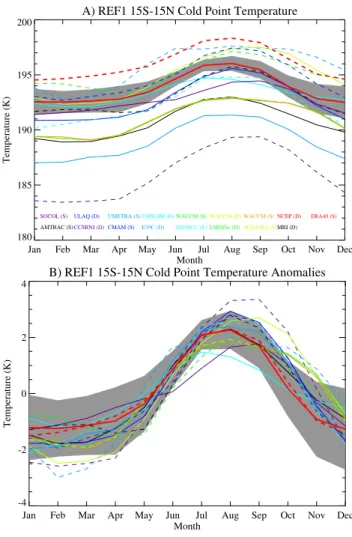
Fig. 2. Annual Cycle of Tropical (15 S–15 N) Zonal mean Cold Point Temperature (TCPT) from REF1 (1979–2001) scenarios of CCMVal Models. (A) Temperature. (B) Temperature anomalies (annual mean removed). Thick Red lines are NCEP/NCAR (dot-ted) and ERA40 (solid) Reanalysis. Gray shading is ±2 standard deviations from ERA40. Models are either solid (S) or dashed (D) lines as indicated in the legend.
3 Multi-model climatology
First we show a few examples of the climatology from the multi-model ensemble from the historical scenarios to ver-ify that CCMs beyond WACCM and CMAM analyzed by GB2007 reproduce the basic structure of the TTL.
Figure 2 illustrates the mean annual cycle of tropical TCPT
for 1980–2000. The full field is shown in Fig. 2a and anoma-lies about the annual mean (highlighting the annual cycle) are shown in Fig. 2b. Models are shown with solid (S) or dashed (D) lines as indicated in the legend for Fig. 2a. The analysis is nearly the same as that for 100 hPa Temperatures shown in Fig. 7 of Eyring et al. (2006). The amplitude of the annual cycle of TCPT(4 K) is similar to the annual cycle amplitude
of 100 hPa temperatures (4 K) in ERA40, and the seasonality is the same.
All models have the same annual cycle of TCPT(Fig. 2b),
to the extent that the peak-to-peak amplitude is 3–5 K with a minimum in December–February and a maximum
in August–September. This is also true for the Lapse
Rate Tropopause Temperature (not shown). Tropical mean TCPTis lowest in December–March, and highest in August–
September. There are some models in which the annual cycle is shifted by 1–2 months relative to the reanalysis (red lines in Fig. 2). The amplitude of annual cycle is 4–5 K in most mod-els (Fig. 2b), but the absolute value varies by 10 K (Fig. 2a). Note that the analysis systems (ERA40 and NCEP) are also different, with NCEP warmer. The differences in analysis systems is due to differences in use of satellite temperature data and radiosonde data (Pawson and Fiorino, 1999). The reasons for the differences in simulated TCPTare likely to be
complex, having to do both with model formulation and the use of monthly mean output. TCPTis analyzed from monthly
mean output on standard levels and may not be relevant for water vapor, since 3-D transport plays a role (see Sect. 5). The difference in TCPT between CCMs is partially due to
slight differences in the pressure of the minimum tempera-ture, which varies similarly to the PLRT (see Fig. 5 below).
GB2007 have shown for WACCM and CMAM overall agree-ment of TCPTand PLRTwith radiosonde and Global
Position-ing System (GPS) radio occultation observations in both the mean and standard deviation.
Differences between 3-D WACCM or 3-D CMAM (cal-culated on model levels using 3-D monthly means) and 2-D WACCM or 2-D CMAM (calculated on standard CCMVal levels using zonal means as input) indicate about 1–2 K tem-perature differences between 2-D and 3-D, (Fig. 1a). Thus for CMAM and WACCM the effect of averaging and inter-polation to standard vertical levels is small. However, the dif-ference makes it somewhat difficult to relate the difdif-ferences in TCPTto differences in water vapor (shown by Eyring et al.
(2006) for these runs). The reanalysis systems have warmer TCPTthan most models, which may be a bias in the analysis
(Pawson and Fiorino, 1999), or due to coarse vertical resolu-tion (Birner et al., 2006). The inter-annual variability, shown as a 2σ confidence interval for the reanalysis in Fig. 2a, is about 2 K.
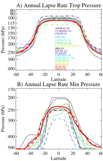
Figure 3a illustrates the annual zonal mean PLRT. The
lapse rate tropopause pressure is a better metric than the cold point tropopause pressure for trends, because in many cases the cold point is always the same level (it is not in-terpolated). TCPTat a constant level occurs when
variabil-ity is less than the model vertical grid spacing. However, we note that TZLR (the cold point interpolated in pressure)
is close to TCPT, and we have also examined PZLR, which
is within 10 hPa of PLRT, and is highly correlated in space
and time. The seasonal cycle is not shown, but the PLRTis
lowest (highest altitude) in February–April (flat in winter), and maximum, (lowest altitude) in July–October. There is more variation seasonally between models, but models are generally clustered with an annual tropical mean of between
A. Gettelman et al.: TTL Trends 1627 92–102 hPa (PLRTis interpolated) and an annual cycle
am-plitude of about 10 hPa. There is more variation between models poleward of 30◦latitude.
The PLRM is illustrated in Fig. 3b. PLRM is generally
around 250 hPa in the deep tropics (15 S–15 N latitude), with 2 models near 200 hPa, and scatter below this. There is lit-tle annual cycle in most models (not shown). PLRMis well
defined in convective regions (see GB2007 for more details) within ∼20◦of the equator. It is not well defined outside of the deep tropics and is not a useful diagnostic there.
4 Long term trends
As noted in Sect. 2.3 we have analyzed trends from WACCM and CMAM with both 3-D and zonal monthly mean data, and found no significant differences in PLRT, TCPTor PLRM. For
WACCM the correlation between 3-D and 2-D annual means is ∼0.96. So for estimating trends, we use the zonal monthly mean data available from all the models. We start with his-torical trends (REF1: 1960–2001) in Sect. 4.1 and then dis-cuss scenarios for the future in Sect. 4.2. Table 3 summarizes multi-model and observed trends for various quantities, with statistical significance (indicated by an asterisk in the table) based on the 2σ (95%) confidence intervals from a bootstrap fit of the multi-model ensemble mean time-series. For the last three columns, not all models provide output over the entire time period (see for example, Fig. 4). Eleven mod-els are included in statistics for REF1 and nine for REF2. E39C and UMETRAC REF2 runs were not available, and the GEOSCCM and MRI values were not included due to double interpolation. ULAQ is not included for analysis of PLRMdue to resolution.
4.1 Historical trends
Little change is evident from 1960–2005 in simulated TCPT
(Fig. 4). It is hard to find any trends which are significantly different from zero in the simulations (Table 3). Some mod-els appear to cool, some to warm, but these do not appear to be significant trends. However, many models and the reanal-ysis systems do indicate cooling from 1991–2004. The result is consistent with Fig. 2 of Eyring et al. (2007) that shows the vertical structure of tropical temperature trends. There is a significant negative trend in TCPTestimated from radiosonde
analyses. NCEP reproduces the trend, but ERA40 does not. However, the NCEP trend may be spurious (Randel et al. (2006), and references therein) resulting from changes in in-put data over time. Thus there is also significant uncertainty in TCPTtrends in the reanalysis data. Radiosonde trends are
considered more robust (Seidel and Randel, 2006).
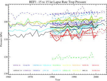
The Lapse Rate Tropopause Pressure (PLRT) does appear
to decrease in the simulations (Fig. 5) and in the reanalyzes, indicating a lower pressure (higher altitude) to the tropical tropopause of −1 to −1.5 hPa/decade (Table 3). However,
A) Annual Lapse Rate Trop Pressure
-60 -40 -20 0 20 40 60 Latitude 400 300 250 200 170 150 130 115 10090 80 Pressure (hPa) AMTRAC (S) CCSRNIES (D) CMAM (S) E39C (D) GEOSCCM (S) LMDZrepro (D) MAECHAM4CHEM (S) MRI (D) SOCOL (S) ULAQ (D) UMETRAC (S) UMSLIMCAT (D) WACCM (S) WACCM (D) WACCM (S) NCEP (D) ERA40 (S)
B) Annual Lapse Rate Min Pressure
-60 -40 -20 0 20 40 60 Latitude 500 400 300 250 200 170 Pressure (hPa)
Fig. 3. Zonal mean (A) Lapse Rate Tropopause Pressure (PLRT) and (B) Lapse Rate Minimum Pressure
(PLRM) from CCMVal models (REF1 scenarios, 1979–2001). Thick Red lines are NCEP/NCAR (dashed) and
ERA40 (solid) Reanalyses. Models are either solid (S) or dashed (D) lines as indicated in the legend in (A). Vertical levels used are noted by tick marks on the vertical axis.
29
Fig. 3. Zonal mean (A) Lapse Rate Tropopause Pressure (PLRT) and (B) Lapse Rate Minimum Pressure (PLRM) from CCM-Val models (REF1 scenarios, 1979–2001). Thick Red lines are NCEP/NCAR (dashed) and ERA40 (solid) Reanalyses. Models are either solid (S) or dashed (D) lines as indicated in the legend in (A). Vertical levels used are noted by tick marks on the vertical axis.
there is no trend in radiosonde analyses of PLRTfrom 1979–
2001. Other analyses with the Parallel Climate Model (San-ter et al., 2003), a subset of these models (Son et al., 2008) and observations (Seidel et al., 2001; Gettelman and Forster, 2002) do show decreases in PLRT. Simulated PLRTtrends are
of the same sign and magnitude as PZLRtrends. In general
the trend is consistent across models in Fig. 5. Inter-annual variability in any model is generally less than in the reanal-yses or radiosondes. As noted, TCPTis correlated with CPT
pressure. The correlation can be seen in the PLRTas well in
Fig. 5: models with lower pressure PLRT have lower TCPT
(Fig. 4).
These tropopause changes represent changes in the “top” of the TTL. The “bottom” of the TTL is represented by the Lapse Rate Minimum pressure (PLRM), which is related to
Table 3. Trends (per decade “d”) in Key TTL quantities from analysis systems (NCEP/NCAR and ERA40) and model simulations. Trends
significantly different from zero (based on 2σ confidence intervals, or 95% level) indicated with an asterix. 13 models are included in statistics for REF1 and 10 for REF2.
Diagnostic Units NCEP/NCAR ERA40 RAOBS Sim REF1 Sim REF1 Sim REF2 Sim REF2 1979–2001 1979–2001 1979–2001 1979–2001 1960–2004 1980–2100 1980–2050 TCPT K/d −0.94∗ 0.54∗ −0.68∗ −0.03 −0.04 0.09∗ 0.09∗ TZLR K/d −1.1∗ 0.53∗ −0.03 −0.03 0.10∗ 0.10∗ PZLR hPa/d −0.28 −0.86∗ −0.58∗ −0.72∗ −0.53∗ −0.60∗ PLRT hPa/d −1.0∗ −1.3∗ 0.0 −0.75∗ −0.66∗ −0.60∗ −0.64∗ PLRM hPa/d −2.8∗ −15∗ −0.36 −2.6∗ −0.25 −2.6∗ −2.3∗
REF1 -15 to 15 lat Cold Point Temperature
1960 1970 1980 1990 2000 Year 180 185 190 195 200 Temperature (K)
AMTRAC (S)CCSRNI (D) CMAM (S) E39C (D) GEOSCC (S) LMDZre (D) MAECHA (S)MRI (D) SOCOL (S) ULAQ (D) UMETRA (S)UMSLIM (D)WACCM (S) WACCM (D)WACCM (S) NCEP (D) ERA40 (S)
RAOB (Dot) REF1 -15 to 15 lat Cold Point Temperature
1960 1970 1980 1990 2000 Year 180 185 190 195 200 Temperature (K)
AMTRAC (S)CCSRNI (D) CMAM (S) E39C (D) GEOSCC (S) LMDZre (D) MAECHA (S)MRI (D) SOCOL (S) ULAQ (D) UMETRA (S)UMSLIM (D)WACCM (S) WACCM (D)WACCM (S) NCEP (D) ERA40 (S)
RAOB (Dot)
Fig. 4. Tropical mean Cold Point Tropopause Temperature (TCP T) from various models for Historical (REF1)
runs. Thin lines are linear trends. Models are either solid (S) or dashed (D) lines as indicated in the legend. Thick red lines are NCEP/NCAR (dashed), ERA40 (solid) Reanalyses and thick red dotted line is radiosonde annual anomalies as described in the text. Thick black line is the multi-model mean anomalies added to the ERA40 inter-annual mean as described in the text.
30
Fig. 4. Tropical mean Cold Point Tropopause Temperature (TCPT) from various models for Historical (REF1) runs. Thin lines are lear trends. Models are either solid (S) or dashed (D) lines as in-dicated in the legend. Thick red lines are NCEP/NCAR (dashed), ERA40 (solid) Reanalyses and thick red dotted line is radiosonde annual anomalies as described in the text. Thick black line is the multi-model mean anomalies added to the ERA40 inter-annual mean as described in the text.
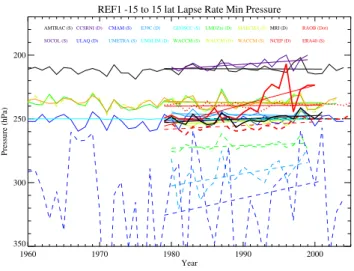
the main convective outflow, and thus a measure of where convection impacts the thermodynamic profile in the TTL. Trends in PLRMare shown in Fig. 6. Large variability and
a higher PLRM in ULAQ is likely due to coarse vertical
(2500 m) and horizontal resolution (10◦×22.5◦).
The multi-model trend in PLRMfor the 1979–2001 is
sig-nificant, with a PLRMdecrease of −2.6 hPa/decade. ERA40
shows a large (−15 hPa/decade) decrease in PLRM, mostly
from 1990–2001. However, radiosondes show no significant trend in PLRM. The reason for the discrepancy in the
analy-sis systems and radiosondes is not known, but may be due to limited radiosonde sampling. The LRM level can vary with unconstrained parts of model convective parameterizations in both CCMs and reanalyses. Thus the diagnostic may not be
REF1 -15 to 15 lat Lapse Rate Trop Pressure
1960 1970 1980 1990 2000 Year 130 120 110 100 90 Pressure (hPa)
AMTRAC (S)CCSRNI (D) CMAM (S) E39C (D) GEOSCC (S)LMDZre (D) MAECHA (S)MRI (D) SOCOL (S) ULAQ (D) UMETRA (S)UMSLIM (D)WACCM (S)WACCM (D)WACCM (S)NCEP (D) ERA40 (S)
RAOB (Dot)
Fig. 5. Tropical mean Lapse Rate Tropopause Pressure (PLRT) from various models for Historical (REF1)
runs. Thin lines are linear trends. Models are either solid (S) or dashed (D) lines as indicated in the legend. Thick red lines are NCEP/NCAR (dashed), ERA40 (solid) Reanalyses and thick red dotted line is radiosonde annual anomalies as described in the text. Thick black line is the multi-model mean anomalies added to the ERA40 inter-annual mean as described in the text.
31
Fig. 5. Tropical mean Lapse Rate Tropopause Pressure (PLRT) from various models for Historical (REF1) runs. Thin lines are lear trends. Models are either solid (S) or dashed (D) lines as in-dicated in the legend. Thick red lines are NCEP/NCAR (dashed), ERA40 (solid) Reanalyses and thick red dotted line is radiosonde annual anomalies as described in the text. Thick black line is the multi-model mean anomalies added to the ERA40 inter-annual mean as described in the text.
quantitatively robust. However, the PLRTin Fig. 5 is much
more tightly constrained, with both analysis systems highly correlated, and many of the models also having correlated inter-annual variability, most likely forced by Sea Surface Temperature patterns (ENSO).
To better understand the above trends, we have analyzed TCPT (Fig. 7a), PLRT (Fig. 7b) and PLRM (Fig. 7c) trends
at each grid point in the REF1 WACCM simulations
us-ing 3-D monthly mean output. The trends are indicated
in Fig. 7, along with trends in cloud top pressure by loca-tion (Fig. 7d). Shaded trends more than one contour inter-val from zero in Fig. 7 are almost always significant at the 95% (2σ ) level. The figure represents an average of trends from all 3 WACCM REF1 realizations, which all have similar patterns. WACCM has moderate correlations with reanalysis
A. Gettelman et al.: TTL Trends 1629 PLRT(Fig. 5), but with less inter-annual variability. WACCM
has less variability because it does not include the aerosol ef-fects of significant volcanic eruptions (such as Mt. Pinatubo in 1991 or El Chichon in 1983).
In Fig. 7a simulated TCPT decreases throughout the
trop-ics in WACCM and increases in the subtroptrop-ics. WACCM simulated TCPTchanges are largest centered over the
West-ern Pacific, but simulated TCPTactually increases over
Trop-ical Africa. The simulated zonal mean trend is not signif-icant. These changes can be partially explained with the pattern of changes in simulated cloud top pressure (Fig. 7d) in WACCM, with decreasing pressure (higher clouds) in the Western Pacific and increasing pressure (lower clouds) in the Eastern Pacific. The clouds appear to shift towards the equa-tor from the South Pacific Convergence Zone (SPCZ), with increasing cloud pressure north of Australia in the WACCM simulations. Figure 7b shows that the simulated PLRT has
decreased almost everywhere in the tropics and sub-tropics, with largest changes in the Eastern Pacific. Simulated PLRM
(Fig. 7c) does not have a coherent trend in WACCM, consis-tent with Fig. 6.
There are very large differences in mean 300 hPa ozone in the tropical troposphere in the models (Fig. 8b). 300 hPa is a level near the ozone minimum. The differences are ex-pected since tropospheric ozone boundary conditions were not specified, and the models have different representations of tropospheric chemistry. The spread of ozone at 300 hPa is 10–80 ppbv with most models clustered around the observed value of 30 ppbv (from SHADOZ Ozonezondes). CMAM ozone (the lowest) is low due to a lack of tropospheric ozone sources or chemistry which may impact TCPT.
Even at 100 hPa near the tropopause there are variations in ozone between 75–300 ppbv (Fig. 8a). The values get larger than the ∼120 ppbv observed from SHADOZ. Most mod-els have a low bias relative to SHADOZ. Several modmod-els are not clustered with the others in Fig. 8a, including LMDZ, MAECHAM, MRI, SOCOL and ULAQ. For MAECHAM this is related to low ascent rates in the lower stratosphere (Steil et al., 2003). There is also a positive correlation (linear correlation coefficient ∼0.6) between average Cold Point Temperature and average ozone in models around the tropopause (150–70 hPa). Models with higher ozone have higher tropopause temperatures in Fig. 2, consistent with an important role for ozone in the radiative heating of the TTL. It may also result from differences in dynamical pro-cesses (slower uplift would imply both higher temperatures and higher ozone). We discuss this further in Sect. 5.
4.2 Future scenarios
We now examine the evolution of the TTL for the future
scenario (REF2). As discussed in Eyring et al. (2007),
the future scenario uses near common forcing for all
mod-els. Models were run from 1960 or 1980 to 2050 or
2100. Surface concentrations of greenhouse gases (CO2,
REF1 -15 to 15 lat Lapse Rate Min Pressure
1960 1970 1980 1990 2000 Year 350 300 250 200 Pressure (hPa)
AMTRAC (S)CCSRNI (D) CMAM (S) E39C (D) GEOSCC (S)LMDZre (D) MAECHA (S)MRI (D) SOCOL (S) ULAQ (D) UMETRA (S)UMSLIM (D)WACCM (S)WACCM (D)WACCM (S) NCEP (D) ERA40 (S)
RAOB (Dot)
Fig. 6. Tropical mean Lapse Rate Minimum Pressure (PLRM) from various models for Historical (REF1) runs.
Thin lines are linear trends. Models are either solid (S) or dashed (D) lines as indicated in the legend. Thick red lines are NCEP/NCAR (dashed), ERA40 (solid) Reanalyses and thick red dotted line is radiosonde annual anomalies as described in the text. Thick black line is the multi-model mean anomalies added to the ERA40 inter-annual mean as described in the text.
32
Fig. 6. Tropical mean Lapse Rate Minimum Pressure (PLRM) from various models for Historical (REF1) runs. Thin lines are linear trends. Models are either solid (S) or dashed (D) lines as indicated in the legend. Thick red lines are NCEP/NCAR (dashed), ERA40 (solid) Reanalyses and thick red dotted line is radiosonde annual anomalies as described in the text. Thick black line is the multi-model mean anomalies added to the ERA40 inter-annual mean as described in the text.
CH4, N2O) are specified from the Intergovernmental Panel
on Climate Change (IPCC) Special Report on Emissions Scenarios (SRES) GHG scenario A1b (medium) (IPCC,
2000). Surface halogens (chlorofluorocarbons (CFCs),
hydro-chlorofluorocarbons (HCFCs), and halons) are pre-scribed according to the A1b scenario of World Meteorolog-ical Organization (2003). Sea surface temperatures (SSTs) and sea ice distributions are derived from IPCC 4th Assess-ment Report simulations with the coupled ocean-atmosphere models upon which the CCMs are based. Otherwise, SSTs and sea ice distributions are from a simulation with the UK Met Office Hadley Centre coupled ocean-atmosphere model HadGEM1 (Johns et al., 2006). See Eyring et al. (2007) for details. Trends in Table 3 are calculated from available data for each model from 1980 to 2050, since only 3 CCMs (AM-TRAC, CMAM, GEOSCCM) are run to 2100. Future trends are broadly linear, and trends for those models run to 2100 are not significantly different if the period 1980–2100 is used (the last two columns are nearly identical. Trends are slightly larger for 2000–2050, likely due to additional forcing from ozone recovery.
Figure 9 illustrates changes in TCPT, similar to Fig. 4 but
for the future (REF2) scenario. Models generally project cold point or lapse rate tropopause temperatures to increase slightly. The multi-model rate of temperature increase is only 0.09 K/decade (Table 3), but is significant. For AMTRAC, the increase is almost 0.3 K/decade in the early part of the 21st century. The increase may be related to the low ozone at the tropopause (Son et al., 2008). The analysis is consistent
A) 1960-2004 TCPT Trend (K/decade) -0.15 -0.05 -0.05 0.10 0.10 0.1 0 B) 1960-2004 PLRT Trend (hPa/decade) -0.5 -0.5 -0.5 -0 .5 C) 1960-2004 PLRM Trend (hPa/decade) -2 -2 -2 -2 -2 -2 4
D) 1960-2004 Cloud Top Press Trend (hPa/decade)
-21 -7 -7 -7 -7 -7 -7 14 14 30N 30S 15N 15S 0 30N 30S 15N 15S 0 0 90 180 270 0 0 90 180 270 0
Fig. 7. Map of trends from historical (REF1) WACCM simulations. Figure shows average of trends from 3
simulations. A) Cold Point Tropopause Temperature (T
CP T) trends, contour interval 0.05K/decade. B) Lapse
Rate Tropopause pressure (P
LRT) trends, contour interval 0.5hPa/decade C) Lapse Rate Minimum Pressure
(P
LRM) trends, contour interval 2hPa/decade. D) Cloud Top Pressure trends, contour interval 7hPa/decade.
Dashed lines are negative trends, no zero line.
A) REF1 -15 to 15 lat 100 hPa Ozone
1960 1970 1980 1990 2000 Year 50 100 150 200 250 300 350 400 Ozone (ppbv)
AMTRAC (S)CCSRNI (D) CMAM (S) E39C (D) GEOSCC (S) LMDZre (D) MAECHA (S)MRI (D)
SOCOL (S) ULAQ (D) UMETRA (S)UMSLIM (D) WACCM (S) WACCM (D) WACCM (S)
B) REF1 -15 to 15 lat 300 hPa Ozone
1960 1970 1980 1990 2000 Year 20 40 60 80 100 Ozone (ppbv)
Fig. 8. Tropical mean Ozone from various models at (A) 100hPa and (B)300hPa. Thin lines are linear trends.
Thick black dashed lines are the SHADOZ observed mean from 1998-2005 at these levels. Models are either
solid (S) or dashed (D) lines as indicated in the legend.
33
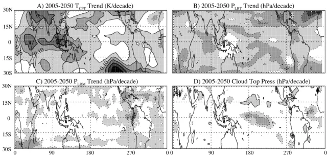
Fig. 7. Map of trends from historical (REF1) WACCM simulations. Figure shows average of trends from 3 simulations. (A) Cold Point
Tropopause Temperature (TCPT) trends, contour interval 0.05 K/decade. (B) Lapse Rate Tropopause pressure (PLRT) trends, contour interval 0.5 hPa/decade (C) Lapse Rate Minimum Pressure (PLRM) trends, contour interval 2 hPa/decade. (D) Cloud Top Pressure trends, contour interval 7 hPa/decade. Dashed lines are negative trends, no zero line.
A) 1960-2004 TCPT Trend (K/decade) -0.15 -0.05 -0.05 0.10 0.10 0.1 0 B) 1960-2004 PLRT Trend (hPa/decade) -0.5 -0.5 -0.5 -0 .5 C) 1960-2004 PLRM Trend (hPa/decade) -2 -2 -2 -2 -2 -2 4
D) 1960-2004 Cloud Top Press Trend (hPa/decade)
-21 -7 -7 -7 -7 -7 -7 14 14 30N 30S 15N 15S 0 30N 30S 15N 15S 0 0 90 180 270 0 0 90 180 270 0
Fig. 7. Map of trends from historical (REF1) WACCM simulations. Figure shows average of trends from 3
simulations. A) Cold Point Tropopause Temperature (TCP T) trends, contour interval 0.05K/decade. B) Lapse
Rate Tropopause pressure (PLRT) trends, contour interval 0.5hPa/decade C) Lapse Rate Minimum Pressure
(PLRM) trends, contour interval 2hPa/decade. D) Cloud Top Pressure trends, contour interval 7hPa/decade.
Dashed lines are negative trends, no zero line.
A) REF1 -15 to 15 lat 100 hPa Ozone
1960 1970 1980 1990 2000 Year 50 100 150 200 250 300 350 400 Ozone (ppbv)
AMTRAC (S)CCSRNI (D) CMAM (S) E39C (D) GEOSCC (S)LMDZre (D) MAECHA (S)MRI (D)
SOCOL (S) ULAQ (D) UMETRA (S)UMSLIM (D)WACCM (S)WACCM (D)WACCM (S)
B) REF1 -15 to 15 lat 300 hPa Ozone
1960 1970 1980 1990 2000 Year 20 40 60 80 100 Ozone (ppbv)
Fig. 8. Tropical mean Ozone from various models at (A) 100hPa and (B)300hPa. Thin lines are linear trends.
Thick black dashed lines are the SHADOZ observed mean from 1998-2005 at these levels. Models are either solid (S) or dashed (D) lines as indicated in the legend.
33
Fig. 8. Tropical mean Ozone from various models at (A) 100 hPa
and (B) 300 hPa. Thin lines are linear trends. Thick black dashed lines are the SHADOZ observed mean from 1998–2005 at these levels. Models are either solid (S) or dashed (D) lines as indicated in the legend.
with Fig. 2 of Eyring et al. (2007) that shows the vertical structure of tropical temperature trends.
In addition to the small temperature increase, simu-lated PLRT decreases as well (altitude increase), seen in
Fig. 10. The rate of decrease of the multi-model ensemble is −0.64 hPa/decade, less than observed during the histori-cal record in REF1 scenarios or observed in the reanalyses
REF2 -15 to 15 lat Cold Point Temperature
1960 1980 2000 2020 2040 2060 2080 2100 Year 180 185 190 195 200 Temperature (K)
AMTRAC (S)CCSRNI (D) CMAM (S) CMAM (D) CMAM (S) GEOSCC (D)MAECHA (S)MRI (D) SOCOL (S) ULAQ (D) UMSLIM (S)WACCM (D)WACCM (S) WACCM (D)
Fig. 9. Tropical mean Cold Point Tropopause Temperature (TCP T) from various models showing expected
future scenarios (REF2). Thin lines are linear trends. Models are either solid (S) or dashed (D) lines as indicated in the legend. Thick black line is the multi-model mean anomalies added to the multi-model inter-annual mean.
34
Fig. 9. Tropical mean Cold Point Tropopause Temperature (TCPT) from various models showing expected future scenarios (REF2). Thin lines are linear trends. Models are either solid (S) or dashed (D) lines as indicated in the legend. Thick black line is the multi-model mean anomalies added to the multi-multi-model inter-annual mean.
(Table 3). However, there is consistency among most of the model trends. All models except one have the same sign of the trend, though with some spread in magnitude (Fig. 10). The ∼15 hPa spread in pressure is likely due to different model formulations and vertical resolution.
A. Gettelman et al.: TTL Trends 1631
REF2 -15 to 15 lat Lapse Rate Trop Pressure
1960 1980 2000 2020 2040 2060 2080 2100 Year 120 115 110 105 100 95 90 Pressure (hPa)
AMTRAC (S)CCSRNI (D)CMAM (S) CMAM (D) CMAM (S) GEOSCC (D)MAECHA (S)MRI (D) SOCOL (S) ULAQ (D) UMSLIM (S)WACCM (D)WACCM (S)WACCM (D)
Fig. 10. Tropical mean Lapse Rate Tropopause Pressure (PLRT) from various models showing expected future
scenarios (REF2). Thin lines are linear trends. Models are either solid (S) or dashed (D) lines as indicated in the legend. Thick black line is the multi-model mean anomalies added to the multi-model inter-annual mean.
35
Fig. 10. Tropical mean Lapse Rate Tropopause Pressure (PLRT) from various models showing expected future scenarios (REF2). Thin lines are linear trends. Models are either solid (S) or dashed (D) lines as indicated in the legend. Thick black line is the multi-model mean anomalies added to the multi-multi-model inter-annual mean.
Figure 11 indicates that the PLRM decreases
signifi-cantly in some simulations (CMAM, WACCM, AMTRAC, MAECHAM), and does not change in others (SOCOL). In some simulations (MRI), the PLRMis not well defined, and
its pressure is indeterminate. In other simulations (CMAM) there are apparent differences in trend before and after 2000.
Since the PLRM represents the impact of convection on
thermodynamics, differences are likely due to different con-vective parameterizations in the simulations. For the multi-model ensemble, the change is −2.3 hPa/decade, and is sig-nificant. Changes in the PLRMindicate changes in the
out-flow of convection in the upper troposphere. The changes in PLRMand PLRTtogether imply a thinner TTL (in mass).
Figure 12 illustrates the map of trends for WACCM from the REF2 runs from 1975–2050. As with Fig. 7, the map is an average of 3 runs with similar patterns. WACCM simu-lated trends in TCPTare smaller than some models (Fig. 9).
WACCM simulated PLRT trends are of similar magnitude
to other models (Fig. 10). Figure 12a indicates that simu-lated TCPT increases in most regions of the tropics.
Sim-ulated TCPT trends are largest (0.2 K/decade) over 0–120 E
(Africa–Indonesia). Simulated TCPT does not change over
the subtropical Pacific. In addition, clouds go up to higher al-titudes, trends up to −14 hPa/decade, over the Central Pacific (Fig. 12d) extending into the Western Pacific. The changes are consistent with 21st century rainfall anomalies in the un-derlying GCM for WACCM (Meehl et al., 2006). These changes are not necessarily consistent in multi-model pro-jections of changes in precipitation (Solomon et al., 2007). The simulated TCPTtrend pattern is consistent with
decreas-ing temperatures from enhanced Central Pacific heatdecreas-ing. The
REF2 -15 to 15 lat Lapse Rate Min Pressure
1960 1980 2000 2020 2040 2060 2080 2100 Year 260 240 220 200 180 Pressure (hPa)
AMTRAC (S)CMAM (D) CMAM (S) CMAM (D) MAECHA (S)UMSLIM (D)WACCM (S)WACCM (D) WACCM (S)
Fig. 11. Tropical mean Lapse Rate Minimum Pressure (PLRM) from various models showing expected future
scenarios (REF2). Thin lines are linear trends. Models are either solid (S) or dashed (D) lines as indicated in the legend. Note that ULAQ is off scale. Thick black line is the multi-model mean anomalies added to the multi-model inter-annual mean.
36
Fig. 11. Tropical mean Lapse Rate Minimum Pressure (PLRM) from various models showing expected future scenarios (REF2). Thin lines are linear trends. Models are either solid (S) or dashed (D) lines as indicated in the legend. Note that ULAQ is off scale. Thick black line is the multi-model mean anomalies added to the multi-model inter-annual mean.
pattern is the same as that observed for the historical record (Fig. 7, see Section 4.1), superimposed on an overall warm-ing.
Simulated PLRT appears to decrease everywhere in the
tropics (Fig. 12b). There is not much structure to the de-crease, though it is larger over the Central Pacific where clouds are going higher in WACCM (Fig. 12d). Simulated PLRM(Fig. 12c) also goes up in most regions of the tropics.
The pattern does not have much structure. There are larger changes near the coast of South America. Simulated changes do not appear to be associated with changes in cloud pressure (Fig. 12d). It may be that another variable would be better suited to looking at coupling between cloud detrainment and the PLRM, but only limited diagnostics are available. These
diagnostics do not indicate as direct a connection between clouds and PLRMchanges as seen in REF1 runs (Fig. 7).
The Zero Lapse Rate (ZLR) pressure (PZLR) and
tempera-ture (TZLR) are another way to examine the thermal structure
around the tropopause. The ZLR is defined identically to the Lapse Rate Tropopause, but for a lapse rate of 0 K/km not −2 K/km. It also defines the cold point, but can be interpo-lated from coarse temperature profiles. The TZLR and PZLR
trends are indicated in Table 3, and are basically identical to TCPT and PLRT trends. TZLR and PZLR trends from the
REF1 scenarios and reanalyses (not shown) are of the same sign (Fig. 4 and Fig. 5). The sign of the trends for TZLR and
PZLRis also the same as TCPTand PLRTtrends for the REF2
scenarios (Figs. 9 and 10). The ZLR trends serve as a con-sistency check on the derived tropopause trends.
A) 2005-2050 TCPT Trend (K/decade) 0.10 0. 10 0.10 0 .10 0.10 B) 2005-2050 PLRT Trend (hPa/decade) C) 2005-2050 PLRM Trend (hPa/decade) 2--2 -2 -2 -2 -2 -2 -2 -2 -2
D) 2005-2050 Cloud Top Press (hPa/decade)
-7 -7 0 90 180 270 0 0 90 180 270 0 30N 30S 15N 15S 0 30N 30S 15N 15S 0
Fig. 12. Map of trends from future (REF2) WACCM simulations. Figure shows average of trends from 3
simulations. A) Cold Point Tropopause Temperature (T
CP T) trends, contour interval 0.05K/decade. B) Lapse
Rate Tropopause pressure (P
LRT) trends, contour interval 0.5hPa/decade C) Lapse Rate Minimum Pressure
(P
LRM) trends, contour interval 2hPa/decade. D) Cloud Top Pressure trends, contour interval 7hPa/decade.
Dashed lines are negative trends, no zero line.
1980 and 2050 T Profiles
185 190 195 200 205 210 Temperature (K) 200 170 150 130 115 100 90 80 70 50 Pressure (hPa) CMAM WACCMFig. 13. Tropical temperature profiles from WACCM and CMAM models for future (REF2) scenarios. Solid
lines: 1980 average. Dashed lines: 2050 average for each of 3 realizations.
37
Fig. 12. Map of trends from future (REF2) WACCM simulations. Figure shows average of trends from 3 simulations. (A) Cold Point Tropopause Temperature (TCPT) trends, contour interval 0.05 K/decade. (B) Lapse Rate Tropopause pressure (PLRT) trends, contour interval 0.5 hPa/decade (C) Lapse Rate Minimum Pressure (PLRM) trends, contour interval 2 hPa/decade. (D) Cloud Top Pressure trends, contour interval 7 hPa/decade. Dashed lines are negative trends, no zero line.
5 Discussion
Finally we address three derived questions that result from these simulations. First, we look at why Cold Point Temper-atures increase but the tropopause rises (decreases in pres-sure) and causes of these changes. Second, we try to use the spread of model ozone values to ask if ozone effects the TTL structure. Third, we look at the implications of tropopause temperature changes on stratospheric water vapor.
5.1 Tropopause changes
It is useful to consider the geometric picture of tropopause trends for an analysis of changes in tropopause tempera-ture given changes in tropopause height (or pressure) and changes in tropospheric and stratospheric temperature, re-spectively. Assume that the temperature profile is piecewise linear and continuous in height with distinct tropospheric and stratospheric temperature gradients 0t and 0s, respectively:
T =0tz+Tsfc for z≤zTP and T =0sz+T0s for z≥zTP. Here,
zTP refers to tropopause height, Tsfc refers to surface
tem-perature and its changes represent tropospheric temtem-perature trends, and T0s is the temperature at which the stratospheric
profile would intersect the ground and its changes repre-sent stratospheric temperature trends. It is straight forward to combine both tropospheric and stratospheric temperature profiles to yield tropopause temperature:
TTP=
0t+0s
2 zTP+
Tsfc+T0s
2 .
Potential trends in tropical tropopause temperature thus result from the combined trends in tropospheric and stratospheric temperatures. Since these are of opposite sign, and the sign changes in the vicinity of the tropopause, it is not clear from simple analytical arguments whether tropopause temperature will increase or decrease. It depends on the bal-ance of the terms in the equation above.
Changes to the TTL given greenhouse gas forcing imply that the tropical tropopause pressure should decrease due to stratospheric cooling or due to tropospheric warming (see
below). However, it is not clear what should happen to
tropopause temperature. If the troposphere warms, the up-per troposphere may warm by a larger amount than the sur-face (Santer et al., 2005). Assuming no change to strato-spheric temperatures, the change would push the tropopause to higher altitudes (lower pressures) and higher temperatures. If the stratosphere cools and the troposphere stays constant, the change would push the tropopause to higher altitudes (lower pressures) and lower temperatures.
In reality, radiative forcing by anthropogenic greenhouse gases both warms the troposphere (increasing Tsfc) and cools
the stratosphere (Solomon et al., 2007). Stratospheric cool-ing will change T0s, depending on the structure and
magni-tude of the temperature change. The changes are illustrated in the vertical profile of temperature trends from these sim-ulations, Fig. 2 of Eyring et al. (2007). The change from warming to cooling is right around the tropopause.
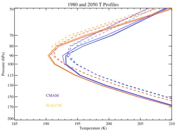
Thus we expect tropopause rises, but what will happen to its temperature? Figure 13 illustrates 1980 (solid) and 2050 (dashed) profiles from WACCM (orange-red) and CMAM
A. Gettelman et al.: TTL Trends 1633 (purple) realizations. Here it is clear that the troposphere is
warming, and the stratosphere is cooling, but the result is a slight warming of the tropopause temperature. The response seems consistent across all model simulations (Fig. 9). As noted by Son et al. (2008) this is dependent upon ozone re-covery, and may be different for those models without inter-active ozone chemistry. We further note that for WACCM
and CMAM, as well as most other models, 0s is
increas-ing in magnitude (more negative) in the stratosphere due to greenhouse gas induced cooling. 0tis increasing in the upper
troposphere at 250 hPa (due to tropospheric warming). The change in sign of the trends is at ≈200 hPa, 100 hPa below the tropopause. The location of the change may imply that over the long term, surface processes (convective equilib-rium) have less of a direct influence on the trends at 150 hPa and lower pressures.
Another way of looking at causes of changes in tropopause height is to do a simple multiple linear regression of TTL di-agnostics on stratospheric temperature and surface tempera-ture. We performed a simple multiple linear regression on annual anomalies of tropical (15 S–15 N) mean TCPT, PLRT
and PLRM, against annual tropical mean anomalies of
strato-spheric (50 hPa) temperature and surface (1000 hPa) temper-ature. We have included ozone concentrations at various lev-els and report those configurations that maximize the fit. The regressions are judged by the percent of variance explained, and individual terms evaluated by the effect on the TTL diag-nostic:◦C (TCPT), hPa (PLRTand PLRM) per standard
devia-tion (σ ) of the predictor (T1000, T50, O3). We have performed
regression on each model time-series included in the multi-model mean for REF2, with available ozone and temperature data: 5 models with 9 realizations: AMTRAC, CMAM (3 realizations), MAECHAM, UMSLIMCAT and WACCM (3 realizations). Regression results are consistent across CCMs. Below we report means across 9 realizations.
Approximately 77% of the interannual variance in tropical averaged TCPTcan be explained by multiple regression with
just 1000 hPa and 50 hPa temperature, and 100hPa Ozone. Where higher T1000, T50 or O3 corresponds to a warmer
tropopause. Surface temperature is the most important
(0.7◦C/σ T1000) followed by 100 hPa Ozone (0.3◦C/σ O3) and
50 hPa temperature (0.2◦C/σ T50). For PLRTa regression with
surface temperature, 50hPa temperature and 100 hPa ozone explains ∼91% of the variance. Higher ozone at 100 hPa implies higher PLRT(0.9 hPa/σ O3) and warmer surface
tem-peratures correlate with lower PLRT (higher tropopause by
−0.7 hPa/σ T1000). Colder stratospheric temperatures
corre-late with higher PLRT (0.4 hPa/σ T50). For PLRM the
sur-face temperatures dominate (81% of interannual variance explained), and an increasing surface temperature causes a decrease in PLRM of −9 hPa/σ T1000. The ozone effect is
smaller, and largest for lower tropospheric ozone (700 hPa: 2.7 hPa/σ O3), and the effect of the stratospheric temperatures
is small (1.5 hPa/σ T50). A) 2005-2050 TCPT Trend (K/decade) 0.10 0. 10 0.10 0 .10 0.10 B) 2005-2050 PLRT Trend (hPa/decade) C) 2005-2050 PLRM Trend (hPa/decade) 2--2 -2 -2 -2 -2 -2 -2 -2 -2
D) 2005-2050 Cloud Top Press (hPa/decade)
-7 -7 0 90 180 270 0 0 90 180 270 0 30N 30S 15N 15S 0 30N 30S 15N 15S 0
Fig. 12. Map of trends from future (REF2) WACCM simulations. Figure shows average of trends from 3
simulations. A) Cold Point Tropopause Temperature (TCP T) trends, contour interval 0.05K/decade. B) Lapse
Rate Tropopause pressure (PLRT) trends, contour interval 0.5hPa/decade C) Lapse Rate Minimum Pressure
(PLRM) trends, contour interval 2hPa/decade. D) Cloud Top Pressure trends, contour interval 7hPa/decade.
Dashed lines are negative trends, no zero line.
1980 and 2050 T Profiles 185 190 195 200 205 210 Temperature (K) 200 170 150 130 115 100 90 80 70 50 Pressure (hPa) CMAM WACCM
Fig. 13. Tropical temperature profiles from WACCM and CMAM models for future (REF2) scenarios. Solid
lines: 1980 average. Dashed lines: 2050 average for each of 3 realizations.
37
Fig. 13. Tropical temperature profiles from WACCM and CMAM
models for future (REF2) scenarios. Solid lines: 1980 average. Dashed lines: 2050 average for each of 3 realizations.
5.2 Ozone impacts on tropopause
Given the wide variation and differences in ozone (Fig. 8), this is a natural experiment to see if ozone matters for the structure of the TTL, as discussed by Thuburn and Craig (2002). It does appear that tropopause level (100 hPa) ozone is correlated with temperature: those models with colder TCPT(Fig. 4) do appear to have less ozone at 100 hPa (Fig. 8),
the correlation between average tropical ozone and TCPT
across 13 models is 0.6. Multiple linear regression dis-cussed above supports the basic correlation, indicating that near tropopause ozone affects both TCPTand PLRT.
It is not clear whether ozone differences are due to trans-port or chemistry. For some models (i.e. CMAM) low ozone is due to missing chemical processes (i.e. lightning NOx pro-duction for CMAM). For other models, slow ascent may allow ozone to increase photochemically (MAECHAM). A positive temperature – ozone correlation might also result from faster (slower) uplift which cools (warms) temperature and decreases (increases) ozone. In addition, models with a colder tropopause have a higher tropopause, but higher (alti-tudes) should have more ozone and more heating, indicating that ozone changes may not be the dominant contributor to observed variability.
5.3 Stratospheric water vapor
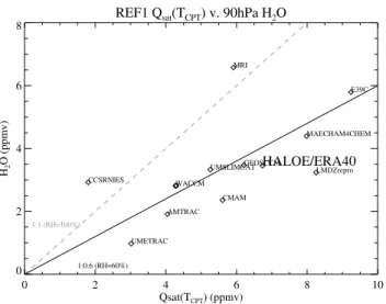
Tropical tropopause temperatures control stratospheric wa-ter vapor (Holton and Gettelman, 2001; Randel et al., 2006). Analysis indicates that the variation in TCPTamong the
mod-els does strongly affect stratospheric water vapor. Figure 14 shows a scatter-plot of the mean annual saturation vapor mix-ing ratio (Qsat) at the TCPT for all the models, plotted as a
function of mean annual 90 hPa water vapor. Also included