Analysis of three-component ambient vibration array measurements

GJI

Seismology

Analysis of three-component ambient vibration array measurements

Donat F¨ah, Gabriela Stamm and Hans-Balder Havenith

Accepted 2007 September 17. Received 2007 September 17; in original form 2006 November 7

S U M M A R Y

Both synthetic and observed ambient vibration array data are analysed using high-resolution beam-forming. In addition to a classical analysis of the vertical component, this paper presents results derived from processing horizontal components. We analyse phase velocities of funda-mental and higher mode Rayleigh and Love waves, and particle motions (ellipticity) retrieved from H/V spectral ratios. A combined inversion with a genetic algorithm and a strategy for selecting possible model parameters allow us to define structural models explaining the data. The results from synthetic data for simple models with one or two layers of sediments suggest that, in most cases, the number of layers has to be reduced to a few sediment strata to find the original structure. Generally, reducing the number of soft-sediment layers in the inversion process with genetic algorithms leads to a class of models that are less smooth. They have a stronger impedance contrast between sediments and bedrock.

Combining Love and Rayleigh wave dispersion curves with the ellipticity of the fundamen-tal mode Rayleigh waves has some advantages. Scatter is reduced when compared to using structural models obtained only from Rayleigh wave phase velocity curves. By adding infor-mation from Love waves some structures can be excluded. Another possibility for constraining inversion results is to include supplementary geological or borehole information. Analysing radial components also can provide segments of Rayleigh wave dispersion curves for modes not seen on the vertical component. Finally, using ellipticity information allows us to confine the total depth of the soft sediments.

For real sites, considerable variability in the measured phase velocity curves is observed. This comes from lateral changes in the structure or seismic sources within the array. Constraining the inversion by combining Love and Rayleigh wave information can help reduce such problems. Frequency bands in which the Rayleigh wave dispersion curves show considerable scatter are often better resolved by Love waves.

Information from the horizontal component can be used to correctly assign the mode number to the different phase–velocity curve segments, especially when two modes seem to merge at osculation points. Such merging of modes is usually observed for Rayleigh waves and thus can be partly solved if additional information from the Love waves and the horizontal component of Rayleigh waves is considered. Whenever a site presents a velocity inversion below the top layer, Love wave data clearly helps to better constrain the solution.

Key words: Time series analysis; Earthquake ground motions; Surface waves and free

oscil-lations; Site effects; Computational seismology; Wave propagation.

1 I N T R O D U C T I O N

Large mountain valleys with wide plains of large fluvial and la-custrine deposits or lakeshores and estuaries with water-saturated sediments are particularly prone to site amplification and non-linear effects. Due to river regulation and engineering progress in the last century, these seismically unfavourable sites have become attrac-tive for expanded settlement and industries. Thus, many villages and cities worldwide have grown extensively into such plains and

are still growing. Given this spread into areas of unfavourable soils, future earthquakes are expected to cause more damage than was observed in the past. To mitigate such effects, we must recognize and map potential areas of damage, estimate ground motion and non-linear behaviour for engineers and planners, and provide ade-quate estimates for building codes. Seismic microzonation studies address these goals, using information from shear wave velocities and geometry of the sediments and the underlying bedrock. Scien-tists in this field also study the possibility of strong non-linear effects

such as liquefaction and landslides. These measured parameters can be used to construct realistic structural models for predicting earth-quake ground motion with numerical techniques. Along with obser-vations of earthquake ground motion from seismic networks, such modelling helps define the local seismic hazard.

Numerical modelling requires good knowledge of the geophysi-cal structure and needs reliable methods to measure physigeophysi-cal param-eters. Ambient vibration techniques have, therefore, become very important in clarifying the eigenvibrations of the geology and es-timating S-wave velocities as a function of depth (e.g. Tokimatsu 1997; Bard 1998; Bonnefoy-Claudet et al. 2006a). This is especially so because they are cheaper and faster than many active methods. However, we need to make ambient vibration methods more reli-able and capreli-able of extracting data contained in recorded ambient vibrations. Traditionally, the vertical component of ambient ground motion has been used to evaluate dispersed Rayleigh waves and de-rive the associated S-wave profile (e.g. Wathelet 2005; Bonnefoy-Claudet et al. 2006a). However, if we analyse all three components of ground motion, ambient vibration techniques have more poten-tial. Here we apply a new method that uses Love and Rayleigh wave phase velocity data and fundamental mode Rayleigh wave ellipticity. It allows us to produce reliable S-wave velocity models. To illus-trate the possibilities and limits of combining such information, we present synthetic and real cases.

1.1 Data sets

The synthetics were computed for two 1-D models with the tech-nique based on wavenumber as proposed by Hisada (1994, 1995); they were provided by the SESAME European project (SESAME Deliverable 12.09.2004; Bonnefoy-Claudet et al. 2006b). The two models are given in Table 1. Noise sources were approximated

Table 1. Models M2.1 and M10.1 used for ambient vibration

simu-lations. M2.1 M10.1 25 m Vp= 500 m s−1 _{31.25 m Vp= 500 m s}−1 Vs= 200 m s−1 _{Vs= 250 m s}−1 Bedrock Vp= 2000 m s−1 375 m Vp= 1800 m s−1 Vs= 1000 m s−1 Vs= 750 m s−1 Bedrock Vp= 3500 m s−1 Vs= 2000 m s−1

by surface forces and randomly distributed in space and time with random direction and amplitude. The time function was ei-ther a frequency-band limited, delta-like signal (impulsive sources) or a pseudo-monochromatic signal (a harmonic carrier with the Gaussian envelope).

Model M2.1 constitutes the simplest case of one layer over a half-space. The second, M10.1, includes two layers over a half-half-space.

Simulations allowed us to select different array geometries of dif-ferent size (shown in Fig. 1). Each array provides information on the dispersion curves over a limited frequency-range related to the size of the array. Small arrays contribute to the dispersion curve at high frequency, large arrays to the dispersion curves at low frequency. The wavenumber range over which each subarray is sensitive is provided later in the examples.

The two real data sets were collected during a measurement cam-paign in the Basel area of Switzerland (Havenith et al. 2007). More than 25 sites were investigated. Different array configurations were tested at different locations. The array geometries of the examples presented here are given in Fig. 2, together with the site locations. The examples shown were selected to investigate the potential of combining Love and Rayleigh wave data.

1.2 H/V spectral ratios

Among several proposed microtremor methods, the H/V technique (Nakamura 1989) has proven very convenient for estimating the fun-damental frequency of soft deposits. Extensive use of this method allows a detailed mapping of this frequency within urban areas. In 1-D structures, average H/V spectral ratios can also be used to esti-mate the ellipticity of the fundamental mode Rayleigh wave (e.g. Ya-manaka et al. 1994). In the P–SV case, ellipticity at each frequency at the free surface is defined as the ratio between the horizontal and vertical displacement eigenfunctions. Ellipticity is detectable in H/V spectral ratios between the peak at the fundamental frequency of res-onance and the first minimum at higher frequency (e.g. F¨ah et al. 2001). The shape of the H/V ratio around its maximum peak can thus be used to estimate a shear wave velocity profile. Yamanaka

et al. (1994), Satoh et al. (2001) and Parolai et al. (2006) applied

this approach to deep sedimentary basins, while F¨ah et al. (2001, 2003) used it for shallow sites. This ellipticity-based method ap-plies only to sites with a high portion of surface waves where strong

S-wave velocity contrast exists between sediments and bedrock, and

1950 2000 2050 2100 2150 1950 2000 2050 2100 2150 M2.1 subarray 1 subarray 2 subarray 3 x [m] y [m] a) 7800 8000 8200 8400 8600 7800 8000 8200 8400 8600 M10.1 subarray 1 subarray 2 subarray 3 x [m] y [m] b)

Figure 1. Geometries of the selected arrays for models M2.1 and M10.1. The array geometries are the same for the two models, but have a different maximum

Figure 2. (a) Basel area in Switzerland, with the location of the measurement sites (stars). Two main tectonic structures can be identified: the Rhinegraben

characterized by thick layers of soft sediments up to 300 m thick in some areas, and the Tabular Jura with a thin cover of Quaternary sediments. (b and c) The geometries of the arrays Kannenfeld and SMZW (Waldhaus) are given by grey circles [the array at Kannenfeld done by Kind (2002) is marked by squares]. Reflection profiles are indicated (dotted line and triangles at end-points).

when sources are near (4–50 times the layer thickness) and close to the surface (Bonnefoy-Claudet et al. 2006b). At such sites, the H/V spectral ratio shows a strong peak.

To constrain the possible solutions, an inversion using a single H/V spectral ratio requires a priori information on the thickness of the sediments. Here ellipticity information is used as an additional constraining quantity for inverting the phase velocity curves.

Two methods are applied to compute average H/V ratios (F¨ah et al. 2001). The first is the classical polarization analysis in the frequency domain, where polarization is defined as ‘the ratio between the quadratic mean of the Fourier spectra of the horizontal components and the spectrum of the vertical component.’ We assume that the vertical component in the frequency band of interest, close to the H/V peak, is dominated by the Rayleigh wave. The SH part of the wavefield contributes to the horizontal component of motion in the measurements. If the SH-part could be removed, the H/V ratios would better determine the ellipticity of the fundamental mode Rayleigh wave. This removal requires some assumptions concerning the spectral content of SH waves. Generally, we assume that the radial component (Rayleigh waves) is equal in amplitude to the transverse (Love waves), and the amplitude of the H/V spectral ratio can then be reduced by log10[sqrt(2)] when the H/V amplitude is given in a logarithmic scale. When a larger contribution of SH waves is noted, the reduction of this H/V curve needs to be stronger. The second method for H/V ratios tries to reduce the SH wave influence by identifying P-SV wavelets from the signal and tak-ing the spectral ratio only from them. This is done by means of a frequency-time analysis (FTAN) on each of the three components of the ambient vibrations. In a frequency-time representation of the vertical signal, the most energetic sections are identified in time for each frequency. We assume that this maximum is related to a single

P-SV wavelet for which the H/V ratio is computed. The average

over all wavelets defines the H/V spectral ratio. For more details

we refer to F¨ah et al. (2001). Since we assume strongly excited fundamental mode Rayleigh waves, this curve will also measure the ellipticity curve. Additionally, this H/V ratio can be used to estimate the SH-wave contribution in a classical H/V ratio computation.

2 A R R AY M E T H O D

The array method we use is based on the high-resolution frequency wavenumber estimator or high-resolution beam-forming (HRBF). It was originally proposed by Capon (1969) but developed and applied to vertical recordings of ambient vibrations by Kind et al. (2005). We have extended this method to analyse the horizontal components. Ambient vibrations recorded on the array are, therefore, analysed for all components of motion. As a prerequisite for a successful measurement, careful placement of the instruments (less than 10◦ error on the orientation with respect to north) is required.

Horizontal ground-motion is analysed for N directions, but to keep the measurement errors to a minimum, N must be large enough: at least 36 to provide a directional resolution of 5◦(180◦/N). This choice gives sufficient resolution for a good analysis. Directional resolution is mostly constrained by the precision with which sensors are oriented in the field. For each direction we compute the ground motion from the two horizontal components and apply HRBF ex-actly as we do for the vertical component (see Kind et al. 2005 for further details). The f –k spectrum is calculated for wavenumber ranges corresponding to a defined velocity range at each frequency, but only for the radial (same direction as the ground motion vector) and transversal (perpendicular to the ground motion vector) parts. By repeating the computation for N directions of ground motion, the

f –k spectrum of the radial (Rayleigh waves) and transverse (Love

waves) components are put together step by step. Finally, for visu-alization, the three f –k spectra for the vertical, radial and transverse

components are converted into a f –c diagram, where c is the phase velocity. A manual interpretation is applied to exclude aliasing and to retrieve a continuous dispersion curve.

The dispersion curves of the fundamental mode and higher mode Rayleigh waves are extracted from the vertical and radial compo-nents of the propagating waves. Love waves are extracted from the transverse component.

In general, arrays with different apertures are set up for the mea-surements to optimize the capabilities in a certain frequency band. Small apertures are used to resolve the shallow part of the struc-ture. By increasing the aperture, deeper and deeper structures can be investigated, and a dispersion curve can be developed over a wide range of frequencies. The HRBF depends on no specific array con-figuration, but the wave-number resolution properties of the array can be optimized through configuration.

The relevant contribution of each array with a certain aperture is the part of the dispersion curve extracted between aliasing at high frequencies and loss of resolution at lower frequencies. The final dispersion curve is defined by combining the respective extracted parts. The selection of the different parts can be checked by com-paring the minimum and maximum wavenumber limits (kminand

kmax) deduced from the theoretical response of each subarray (array with a certain aperture). kmindefines the resolution limit of the array geometry and is measured where the central peak of the theoretical array response reaches mid-height. kmaxdefines the aliasing limit and is set where the first aliasing peak exceeds 0.5. For the real data set ‘Kannenfeld’, we used only the parts between kminand kmax/2, as recommended by Wathelet (2005). For the synthetic data sets and the real data set ‘SMZW’, however, we used the parts between kmin and kmax. A condition for applying the HRBF technique is the intrin-sic assumption of a 1-D-layered medium. The stability of the H/V spectral ratios within the array can be used to validate this assump-tion. For 2-D structures, methods must allow for the interpretation of 2-D resonance phenomena (Steimen et al. 2003; Roten et al. 2006; Roten & F¨ah 2007).

To check the results of our analysis, we independently applied the CAP and SESARRAY software developed during the SESAME project to the vertical component of motion (Ohrnberger 2004; Wathelet 2005). We obtained the same results for the Rayleigh wave dispersion curves.

3 I N V E R S I O N

The inversion scheme is based on a genetic algorithm. This type is generally robust and easily adapted to a specific problem. The genetic algorithm we apply was developed by D. Carroll and is de-scribed in F¨ah et al. (2001, 2003). It does not require explicit starting models: only the definition of parameter limits. The combined H/V spectral ratios and phase velocity curves for Love and Rayleigh waves are used to estimate the average S-wave velocity structure below the array. In this inversion, a number of layers are prescribed and parameter ranges are fixed for the geophysical properties of those layers.

The different segments of the dispersion curves must be assigned to a certain mode. This is a major difficulty in the procedure, since a wrong assignment might result in models far from the real struc-ture. Combining Love and Rayleigh wave dispersion curve segments helps reduce this problem, because inconsistent assignments will show up during the inversion: a bad fit between observed and theo-retical phase velocity curves will stick out.

The initial starting population of possible models is generated through a uniform random distribution in the parameter space. The

ellipticity of the fundamental mode Rayleigh wave and the phase velocities for Love and Rayleigh waves are calculated for the whole population with the modal summation algorithms developed by Panza (1985), Panza & Suhadolc (1987) and Florsch et al. (1991).

For ellipticity (in log10) we use the squared difference between the computed and the measured curve to define the fitness function for the evolution of the population. For each phase-velocity curve segment (in linear scale), we use the absolute difference between computed and measured curves to define its fitness function. Phase velocities range between 0 and 1 km s−1, whereas measured elliptic-ity typically ranges between−1 and 1. The single fitness functions are normalized to range between 0 (bad fit) and 1 (perfect fit). For the combined fitness function, different weights are applied to the functions for the dispersion curve segments with values 1, 2 or 3. For different inversion runs we use different weight combinations. The weight on the ellipticity fitness function is always 1.

Throughout this study a maximum of eight soft sediment layers were used and at least two contrasting layers with higher velocities served as bedrock. Below the bedrock layer, we used a fixed standard structural model for the basement. Starting with eight layers of soft sediments, the number of layers is consecutively reduced to two to five layers with soft sediments.

3.1 Synthetic case I/Model M2.1

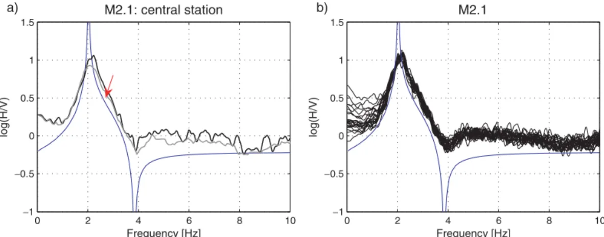
Fig. 3 compares the theoretical ellipticity of the model to classical H/V spectral ratios of the central station and of all stations, respec-tively. In Fig. 3(a), the H/V ratio computed with the FTAN is pre-sented as well (grey curve). Both classical H/V spectral ratios and H/V ratios computed with FTAN are larger than the ellipticity over a wide range of frequencies (red arrow Fig. 3a). The classical H/V spectral ratios were corrected by considering an equal contribution of SH and P–SV waves. However, the synthetic signals are domi-nated by Love waves (Bonnefoy-Claudet et al. 2006b), increasing the SH-contribution in the frequency band of interest for the inver-sion between 2.1 and 4 Hz. Thus, the curves were not sufficiently reduced for classical H/V ratios. This finding is valid for both syn-thetic examples presented here but is generally not observed at real sites (where an equal contribution of SH and P–SV can often be as-sumed). As shown in Fig. 3, the effect of the dominating Love-waves could not be completely removed from the H/V curves by the FTAN method. This fact will influence the inversion results shown later. The strong peak at the fundamental frequency of resonance at about 2.1 Hz is a result of a strong velocity contrast between sediments and bedrock.

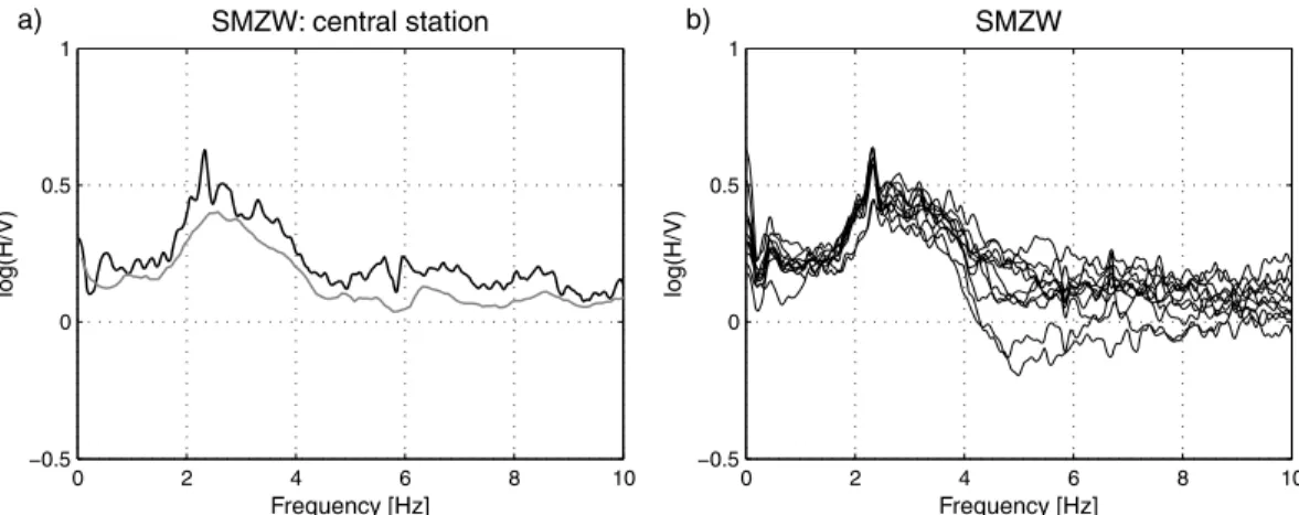
The analysis of the array data resulted in the dispersion curves shown in Fig. 4. Processing the vertical and radial components pro-vided the dispersion curve for the fundamental mode Rayleigh wave, and the radial component also showed a series of dispersion curve segments of higher modes (Fig. 4a). The dispersion curve for the fundamental mode Love wave was retrieved over a large frequency band from the transverse component (Fig. 4b). Higher modes could not be extracted. The dispersion curves were finally interpolated to a regular sampling in the frequency domain so that they could be used for inversion (Figs 4c and d).

For the inversion, different segments of the dispersion curves have to be selected. Due to the more scattered points retrieved from the radial component, only the picked points from the vertical compo-nent were used to define the dispersion curve of the fundamental mode Rayleigh wave. The larger scatter is most probably due to the dominant Love wave energy on the horizontal component. Segments

0 2 4 6 8 10 −1 −0.5 0 0.5 1 1.5 log(H/V) Frequency [Hz] M2.1: central station a) 0 2 4 6 8 10 −1 −0.5 0 0.5 1 1.5 log(H/V) Frequency [Hz] M2.1 b)

Figure 3. (a) H/V spectral ratio obtained for the central station of array M2.1. The black line is the result from classical polarization analysis in the frequency

domain and corrected for SH waves. We assumed equal amplitude of SH and P–SV waves on the horizontal components. The grey line was obtained with the method based on frequency-time analysis. The blue curve is the ellipticity of the fundamental mode Rayleigh wave of model M2.1. The difference between the H/V curves and the ellipticity indicates a strong contribution of SH and Love waves (red arrow). (b) Comparison of the H/V spectral ratios of all stations in the array using classical polarization analysis.

0 5 10 15 0 200 400 600 800 1000 vertical ( • ), radial ( + ) frequency [Hz] c [m/s] subarray 1 subarray 2 subarray 3 0 ₁ 2 a) 0 5 10 15 0 200 400 600 800 1000 transverse ( ♦ ) frequency [Hz] c [m/s] subarray 1 subarray 2 subarray 3 0 1 b) 0 5 10 15 0 200 400 600 800 1000 frequency [Hz] c [m/s] c) 0 5 10 15 0 200 400 600 800 1000 frequency [Hz] c [m/s] d)

Figure 4. Dispersion curves for Rayleigh (a, c) and Love waves (b, d). Vertical: analysis of the vertical components; radial: analysis of the radial components;

transverse: analysis of the transverse components. The dispersion curves obtained from the array analysis (different colours for the subarrays) are compared to the theoretical curves (black). The numbers indicate the mode number (0: fundamental mode; 1: first higher mode, 2: second higher mode). kminand kmaxof the subarrays are given, respectively, as dashed and dash-dotted lines and define the resolution limit of the subarray geometries. (a) and (b) manually picked dispersion curves compared to the theoretical curves. (c) and (d) Segments used for the inversion (red), compared to the theoretical curves.

with low scatter of the picked points were used for the inversion and are shown in Figs 4c and d. In a first step of the inversion, we have used only the dispersion curve segments of the Rayleigh wave fun-damental mode dispersion curve, simulating the classical procedure of inverting only those segments obtained from the vertical com-ponent of motion. Different runs were characterized by different

weights applied to the dispersion curve segments, a different num-ber of layers and different allowed parameter ranges. The resulting structural models are given in Fig. 5(a) as blue curves. The entire set of solutions defines the uncertainties. In the inversion the veloc-ity of the soft-sediment layer is retrieved. However, the thickness of the layer is resolved with limited accuracy. The velocity of the

0 400 800 1200 1600 2000 0 20 40 60 80 100 v_s [m/s] depth [m]

*

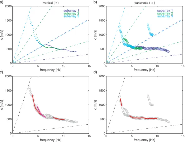
Figure 5. Inverted models (colours) compared to model M2.1 (black). The black line shows the true model. (a) The blue structures are obtained using only

Rayleigh wave dispersion curve segments for the inversion. (b) The green models show the resulting structures when Love and Rayleigh wave dispersion curves and the information from the H/V ratios are included in the inversion with four sediment-layers. (c) Red curves represent structures obtained by the same method as in (b) but considering only one sediment layer.

bedrock cannot be determined due to missing information in the phase velocity curves used. In the inversion, the S-wave velocity of the bedrock generally tends to very high values.

In a second step, the different segments of the Love and Rayleigh wave dispersion curves and the H/V ratio were used and weighted differently in single inversion runs. The weights on the dispersion curve segments are 1, 2 or 3; the weight on the H/V ratios is always 1. This results in different possible models which Fig. 5(b) shows in green. The different weights do not significantly change the data misfit. The scatter is reduced when compared to that in the structural models obtained from Rayleigh wave phase velocity curves only. The velocity of the bedrock layer and the thickness of soft sediments can be resolved slightly better than in the previous case but with limited accuracy. The combined use of all information does slightly improve the solution in this example.

In a third step, the number of sediment layers in the model was reduced to one, as in the theoretical model (red curves in Fig. 5c). With the reduced number of layers, a very good fit was found. These models are preferred due to the reduction in free parameters. The thickness of the sediment layer is now resolved to considerable accuracy.

Fig. 6 shows both the fit of the dispersion curves and the ellip-ticities of the inverted models compared to the theoretical curves of model M2.1. The fit is good in the selected segments for the in-version, but it shows some deviation in the other frequency band where no data was used for the inversion. This is especially true for the dispersion curves at lower frequencies below about 2 Hz. Additional constraints would be needed to improve the results for this frequency band.

Even for inversions in which no Love wave information is used (blue curves in Fig. 6b), the fit between the true dispersion curve and the ones for the inverted models is very good. The only excep-tion (labelled with (∗) in Fig. 5a) is a structure with a thick layer of soft sediment and very high-velocity bedrock, far away from the real structure. We can exclude such structures by using Love wave information. A general observation is that after combining data the bedrock of the inverted structure is much closer to the real model.

We conclude from this test that introducing additional informa-tion (here the knowledge of the number of sediment layers) improves the result of the inversion for the sediments much more than using only Love and Rayleigh wave phase velocity combined with H/V data. This conclusion is only true for synthetic cases in which no variability of the measured phase velocity curves is introduced due to lateral changes of the structure or seismic sources within the array.

Such sources can be anthropogenic, structural features, or buildings that scatter the incident ambient vibration wavefield. In real cases, constraining the inversion through Love and Rayleigh wave data helps reduce uncertainties.

3.2 Synthetic case II/Model M10.1

Model M10.1 is treated in the same way as the previous example. However, here the dispersion curves of the Rayleigh waves show a more complex pattern (Fig. 7). The dispersion curves of different modes are very close to each other at about 3.5 Hz. This oscula-tion point might cause difficulties in real cases, where data could be attributed to the wrong mode and thus misinterpreted (mode jumping). The picks of the radial component in the frequency band 2–3 Hz indicate that an average velocity of the fundamental mode and the first higher mode is measured. In cases where two modes are excited and not sufficiently separated in time, distinguishing the two dispersion curves is not possible (mode mixing). Analysing the ra-dial component provides the phase velocity curve of the first higher mode for frequencies above 4 Hz. Due to larger scatter, this segment was not used for the inversion. The fundamental mode Love wave can be detected over a broad range of frequencies and helps in inter-preting the dispersion curves in the Rayleigh wave case. However, the phase velocity curve obtained with HRBF for the fundamental mode Love wave differs from the theoretical curve in the frequency band between 1 and 1.5 Hz. This difference will influence the re-sult of the inversion. For the inversion, only selected segments of the Rayleigh wave dispersion curves are used (first higher mode 2–3 Hz, fundamental mode around 1 Hz and in the range 4–7 Hz) together with the fundamental mode Love wave dispersion curve (see Figs 7c and d).

Again we used only the dispersion curve segments of the Rayleigh waves obtained from the vertical component of motion by cor-rectly assigning the mode number to all segments. Different runs were characterized by different weights applied to the dispersion curve segments, a different number of layers and different param-eter ranges. These selections do not significantly change the data misfit. The resulting structural models are given in Fig. 8(a) as blue curves. The misfit to the dispersion curves and ellipticity is given in Fig. 9.

The entire set of solutions defines the uncertainties. The scatter becomes larger with increasing depth, because no information is contained in the phase velocity curves for velocities larger than

0 5 10 15 0 200 400 600 800 1000 Frequency [Hz] Phase v elocity [m/s ] a1) 0 5 10 15 0 200 400 600 800 1000 Frequency [Hz] M2.1: Rayleigh a2) 0 5 10 15 0 200 400 600 800 1000 Frequency [Hz] a3) 0 5 10 15 0 200 400 600 800 1000 Frequency [Hz] Phase v elocity [m/s ] b1) 0 5 10 15 0 200 400 600 800 1000 Frequency [Hz] M2.1: Love b2) 0 5 10 15 0 200 400 600 800 1000 Frequency [Hz] b3) 0 2 4 6 8 10 0 1 2 Frequency [Hz] Ellipticity c1) 0 2 4 6 8 10 2 1 0 1 2 Frequency [Hz] c2) M2.1: Ellipticity 0 2 4 6 8 10 2 1 0 1 2 Frequency [Hz] c3)

Figure 6. (a, b) Comparison between dispersion curves of the inverted structural models (colour) and theoretical curves for Rayleigh (a) and Love waves (b)

for model M2.1 (black). The end-points of the segments used for the inversion are shown by arrows. The blue curves (a1, b1) are for the structures obtained using only Rayleigh wave dispersion-curve segments for the inversion. The green (a2, b2: structure with four sediment-layers) and red curves (a3, b3: structure with one sediment layer) show the dispersion curves of the inverted structures when Love and Rayleigh wave dispersion curves and the data from the H/V ratio are included. (c) Comparison between ellipticities of the fundamental mode Rayleigh wave and the ellipticity of the theoretical model M2.1(shown in black).

about 1000 m s−1. As in the M2.1 case, the velocity of the bedrock in the inversion tends to be high.

In a second step, we used different segments of the Love and Rayleigh wave dispersion curves and the H/V ratio and weighted them differently in single inversion runs, as in the first example. The weights on the dispersion curve segments are 1, 2 or 3; the weight on the H/V ratios is always 1. This choice results in different possible models shown in Fig. 8(b) in green and Fig. 8(c) in red. By including several soft-sediment layers in the inversion (green structures in Fig. 8b), the resulting structures are smoothed when compared to the real structure. The two-layer over bedrock character is recovered, but we cannot define the deeper velocity contrast at 400 m depth or the bedrock’s S-wave velocity. By combining Love and Rayleigh wave phase velocity curves and ellipticity of the fundamental mode Rayleigh wave, we reduce slightly the scatter of the results.

Reducing the number of soft-sediment layers to 2 leads to a class of less smooth models which fit the theoretical structure (two sed-iment layers, Fig. 8c) better. To cover all models that explain the observed dispersion curves, such layer reduction is, therefore, rec-ommended. The misfit to the theoretical curves is equally good for the multilayer and two-layer models (Fig. 9). However, inversions

with the exact number of sediment layers converge to more stable solutions with less scatter than in the multilayer case.

In this example data from the radial component has been used only to correctly assign mode numbers to the different segments. Given the larger scatter for the radial components, we have not used these segments for the inversion. The phase velocity curve of the first higher Rayleigh mode for frequencies above 4 Hz would add useful information. Without data from the horizontal component (Love and Rayleigh wave dispersion curves), a correct assignment of the mode number to the different segments would have been difficult. This is a very important advantage in using horizontal components.

3.3 Real site I/Site Waldhaus-SMZW

The first real site is located in the area outside the Rhinegraben. No large roads or industries are within a distance comparable to the array aperture, so the approximation of plane wave-fields is appropriate. The geology down to the bedrock is well known from boreholes. The site is characterized by about 35–40 m of Quaternary gravels above the bedrock consisting mostly of Triassic chalks with some

0 2 4 6 8 10 0 500 1000 1500 vertical ( • ), radial ( + ) frequency [Hz] c [m/s] subarray 1 subarray 2 subarray 3 0 1 a) 0 2 4 6 8 10 0 500 1000 1500 transverse ( ♦ ) subarray 1 subarray 2 subarray 3 frequency [Hz] c [m/s] 0 1 b) 0 2 4 6 8 10 0 500 1000 1500 frequency [Hz] c [m/s] c) 0 2 4 6 8 10 0 500 1000 1500 frequency [Hz] c [m/s] d)

Figure 7. Dispersion curves for Rayleigh (a, c) and Love waves (b, d) in the case of Model M10.1. Vertical: analysis of the vertical components; radial:

analysis of the radial components; transverse: analysis of the transverse components. The dispersion curves obtained from the subarray analysis (different colours for the subarrays) are compared to the theoretical curves (black). The numbers indicate the mode number (0: fundamental mode; 1: first higher mode). kminand kmaxof the subarrays are given, respectively, as dashed and dash-dotted lines and define the resolution limit of the subarray geometries. (a) and (b) Manually picked dispersion curves compared to the theoretical curves. (c) and (d) Segments used for the inversion (red) compared to the theoretical curves. 0 500 1000 1500 2000 2500 0 200 400 600 v_s [m/s] depth [m] a) 0 500 1000 1500 2000 2500 0 200 400 600 v_s [m/s] M10.1 b) 0 500 1000 1500 2000 2500 0 200 400 600 v_s [m/s] c)

Figure 8. Inverted models (colour) compared to Model M10.1 (black). The black line shows the true model. (a) The blue structures are obtained using only

Rayleigh wave dispersion-curve segments for the inversion (b) The green curves show the resulting structures when Love and Rayleigh wave dispersion curves and information from the H/V ratios are included in the inversion with seven to eight sediment layers; (c) red curves, the same as (b) representing structures with only two sediment layers.

small graben structures of Keuper and Lias (having a width of a few hundred of metres or kilometres—see also grey fault lines in Fig. 2). The top of the bedrock is known to be strongly weathered. The approximation of horizontal layering applies well to the site, and the topography is flat. The hypothesis of the 1-D medium is verified by comparing the H/V spectral ratios of the central station (Fig. 10a) with those of the other stations (Fig. 10b). This compari-son shows that the H/V ratios are quite similar within the array. The curves are very uniform below about 4 Hz, but vary slightly in the

higher frequency range. The clear, high-amplitude peak at 2–3 Hz indicates a strong S-wave velocity contrast between sediments and bedrock. The differences between the different H/V curves above 4 Hz suggest slight lateral variations of the surface layer in the al-luvial gravels.

Analysis of the three subarrays with 20, 50 and 100 m radius (Fig. 2c) resulted in the dispersion curves shown in Figs 11(a) and (b). For the inversion analysis we used only the red and pink seg-ments of dispersion curves produced from the vertical and transverse

0 2 4 6 8 10 0 500 1000 1500 Frequency [Hz] Phase v elocity [m/s ] a1) 0 2 4 6 8 10 0 500 1000 1500 Frequency [Hz] M10.1: Rayleigh a2) 0 2 4 6 8 10 0 500 1000 1500 Frequency [Hz] a3) 0 2 4 6 8 10 0 500 1000 1500 Frequency [Hz] Phase v elocity [m/s ] b1) 0 2 4 6 8 10 0 500 1000 1500 Frequency [Hz] M10.1: Love b2) 0 2 4 6 8 10 0 500 1000 1500 Frequency [Hz] b3) 0 2 4 6 8 10 0 1 2 Frequency [Hz] Ellipticity c1) 0 2 4 6 8 10 2 1 0 1 2 Frequency [Hz] M10.1: Ellipticity c2) 0 2 4 6 8 10 2 1 0 1 2 Frequency [Hz] c3)

Figure 9. (a, b) Comparison between dispersion curves of the inverted structural models (in colour) and theoretical curves for Rayleigh (a) and Love waves (b)

for model M10.1 (black). The end-points of the segments used for the inversions are shown by arrows. The blue curves (a1, b1) are for the structures obtained using only Rayleigh wave dispersion-curve segments for the inversion (dark blue: fundamental mode; light blue: first higher mode), the green/brown (a2, b2: structure with seven to eight sediment-layers) and red/magenta curves (a3, b3: structure with two sediment layers) show the dispersion curves of the inverted structures when Love and Rayleigh wave dispersion curves and the information from the H/V ratio are included (green and red: fundamental mode; brown and magenta: first higher mode). (c) Comparison between ellipticities of the fundamental mode Rayleigh wave and the ellipticity of the theoretical model M10.1 (shown in black). 0 2 4 6 8 10 5 0 0.5 1 log(H/V) Frequency [Hz] SMZW: central station a) 0 2 4 6 8 10 0.5 0 0.5 1 log(H/V) Frequency [Hz] SMZW b)

Figure 10. (a) H/V spectral ratios obtained for the central station for array at site SMZW. The black line is the result of classical polarization analysis in the

frequency domain and corrected for SH waves using the assumption of equal amplitude of SH and P-SV waves on the horizontal components. The grey line is obtained with the method based on frequency-time analysis. (b) Comparison of the H/V spectral ratios of all stations in the array using classical polarization analysis.

0 5 10 15 0 500 1000 1500 2000 vertical ( • ) frequency [Hz] c [m/s] subarray 1 subarray 2 subarray 3 a) 0 5 10 15 0 500 1000 1500 2000 transverse ( ♦ ) frequency [Hz] c [m/s] subarray 1 subarray 2 subarray 3 b) 0 5 10 15 0 500 1000 1500 2000 frequency [Hz] c [m/s] c) 0 5 10 15 0 500 1000 1500 2000 frequency [Hz] c [m/s] d)

Figure 11. Measured dispersion curves for Rayleigh (a, c) and Love waves (b, d). Vertical: analysis of the vertical components; radial: no useful segments were

found; transverse: analysis of the transverse components. kminand kmaxof the subarrays are given, respectively, as dashed and dash-dotted lines and define the resolution limit of the subarray geometries. (a) and (b) Manually picked dispersion curves. (c) and (d) Segments used for the inversion (two possible variants for the fundamental mode Rayleigh wave for the frequency band around 5 Hz are tested: red and pink).

components (see Figs 11c and d, respectively). The radial component provided no useful dispersion curve segments. At first glance, the two branches between 5 and 7 Hz might be the fundamental mode and the first higher mode dispersion curve, or a superposition of fundamental and higher modes. The fundamental mode Love wave can be extracted from all arrays, except for the frequency range 3.5–4.5 Hz in which considerable scatter is observed. The inver-sion results provided a much better fit when the observed higher-frequency segment of the Rayleigh wave dispersion curve was assigned to the fundamental mode. We show here only these solutions.

As expected, scatter in the dispersion curves chosen is larger than for the synthetic cases, reflecting the non-ideal measurement and environmental conditions. This uncertainty could be quantified by using different possible dispersion curve segments as input to the inversions.

For the inversion, both the dispersion curves segments and the H/V spectral ratio were used. A series of inversion runs were car-ried out, with various weights attributed to the different segments of the dispersion curves and the H/V ratio. The weights and allowed parameter ranges were selected similarly as with the synthetics. For the inversion, we first used both the Rayleigh wave dispersion curve segments and the ellipticity data. The models resulting from this inversion are shown in Fig. 12(a) as blue curves. The entire set of solutions defines the uncertainties. At the same site, S-wave re-flection seismic measurements were performed (Polom et al. 2005; profile end points shown by triangles in Fig. 2c). The results from the seismic measurement confirm the results of the array

investi-gations. The structural details in the shallow part of the structures down to about 20 m might be real features of the site, but this infor-mation is not contained in the dispersion curve segments used for the inversion.

Then, the Love wave dispersion curves were added for the inver-sion (green and red structures in Fig. 12b). The additional Love data does not dramatically change the results of the inversion, but pro-vides a new class of models. With the reduced number of layers, we also found a good fit between measured and inverted curves. The green curves are the models with the lowest number of sediment layers (two layers) that still result in a good fit. The structures are comparable to the previously obtained results using an increased number of layers. Since we do not know the true model, we cannot decide whether layer reduction is required. Using more geophysical layers than lithological units may be justified by the presence of a velocity gradient within the same unit. This was shown by Havenith

et al. (2007), clearly resolving a velocity gradient within the gravel

layers in our investigation area. The increase of the velocity with depth is due to compaction of the material. Weathering of a litho-logical unit might cause a reduction of the velocity in its upper part. An example is the Meletta layer discussed in the following section for site Kannenfeld.

Fig. 13 shows how the dispersion curves and ellipticities of the inverted models fit the measured curves at site SMZW. The Love wave dispersion curves, for all cases that used Love wave infor-mation in the inversion, always provide a good fit to the observed data. For some models the fit to the observed Rayleigh wave dis-persion curve at high frequency is also satisfactory. All ellipticity

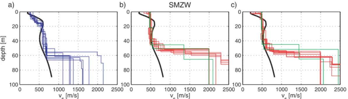
0 500 1000 1500 2000 2500 0 20 40 60 80 100 v_s [m/s] depth [m] a) 0 500 1000 1500 2000 2500 0 20 40 60 80 100 v_s [m/s] SMZW b) 0 500 1000 1500 2000 2500 0 20 40 60 80 100 v_s [m/s] c)

Figure 12. Inverted models (colour) compared with results from seismic reflection (black, by Polom et al. 2005). (a) The blue structures are obtained using only

Rayleigh wave dispersion-curve segments and the ellipticity for the inversion. (b) The green and red curves show the resulting structures when the information from the Love waves is included in the inversion. The red curves represent structures allowing four to seven soft sediment-layers; for the green structures, only two were allowed. (c) The same as (b) but using an alternative segment around 5 Hz (pink segment in Fig. 11c) for the Rayleigh wave phase velocity.

0 5 10 15 0 500 1000 1500 2000 Frequency [Hz] Phase v elocity [m/s ] a1) 0 5 10 15 0 500 1000 1500 2000 Frequency [Hz] SMZW: Rayleigh a2) 0 5 10 15 0 500 1000 1500 2000 Frequency [Hz] a3) 0 5 10 15 0 500 1000 1500 2000 Frequency [Hz] Phase v elocity [m/s ] b1) 0 5 10 15 0 500 1000 1500 2000 Frequency [Hz] SMZW: Love b2) 0 5 10 15 0 500 1000 1500 2000 Frequency [Hz] b3) 0 2 4 6 8 10 5 5 0 0.5 1 1.5 Frequency [Hz] Ellipticity c1) 0 2 4 6 8 10 1.5 1 0.5 0 0.5 1 1.5 Frequency [Hz] SMZW: Ellipticity c2) 0 2 4 6 8 10 1.5 1 0.5 0 0.5 1 1.5 Frequency [Hz] c3)

Figure 13. (a, b) Comparison between dispersion curves of the inverted structural models and the observed curves (black) for Rayleigh (a) and Love waves

(b). (a1, b1) The blue curves are obtained using only Rayleigh wave dispersion-curve segments and the ellipticity for the inversion. (a2, b2) The green and red curves show the resulting structures when the information from the Love waves is included in the inversion. The red curves represent structures allowing four to seven soft sediment-layers; for the green structures, only two were allowed. (a3, b3) The same as (a2, b2) but using an alternative segment around 5 Hz (pink segment in Fig. 11c) for the Rayleigh wave phase velocity. (c) Comparison between ellipticities of the fundamental mode Rayleigh wave and the observed H/V ratios computed for the central station of the array. The end-points of the segments used for the inversion are shown by arrows.

curves of the models roughly fit the observed right flank of the H/V curve, which was used as a target in the inversion process. All in-versions, however, show a poor fit to the observed Rayleigh wave dispersion curve at low frequency. This might indicate a problem

with that segment of the measured dispersion curve. When looking at Fig. 11, we see for the Rayleigh wave phase velocity an alternative segment around 5 Hz (pink segment) that better fits the theoretical curves from the inverted models. Repeating the inversions using

this segment leads to the structures shown in Fig. 12(c), with the fit between measured and inverted curves shown in Figs 13a3, b3 and c3.

3.4 Real site II/Site Kannenfeld

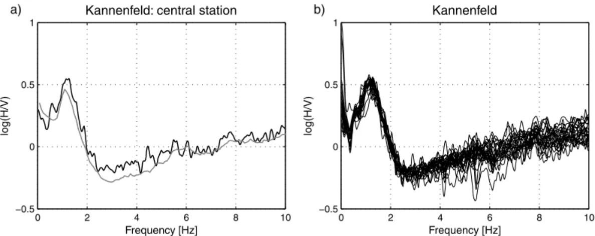
Kannenfeld is located within a park in the city of Basel. This site has been investigated by Kind (2002) and Havenith et al. (2007); both used ambient vibration array measurements on the vertical component of motion. Polom et al. (2005) applied S-wave reflec-tion at about 200 m from the array centre. The site is character-ized by soft quaternary deposits (gravels) with a thickness of about 5–20 m. The gravels can be cemented over certain depth intervals. Below the quaternary sediments, we find thick Meletta layers (100– 150 m): a soft argillaceous material. The upper part of the Meletta layer is weathered. The bedrock (Sannoisien) is reached at about 150 m depth. The 1-D structure of this site with four main geo-logical layers is verified by similar H/V spectral ratios at the array stations (Fig. 14). The measured dispersion curves of Rayleigh and Love waves are given in Fig. 15. Note the high velocities of the Love waves (700–1000 m s−1) compared to those of Rayleigh waves (450–1000 m s−1) in the frequency band between 2 and 4 Hz.

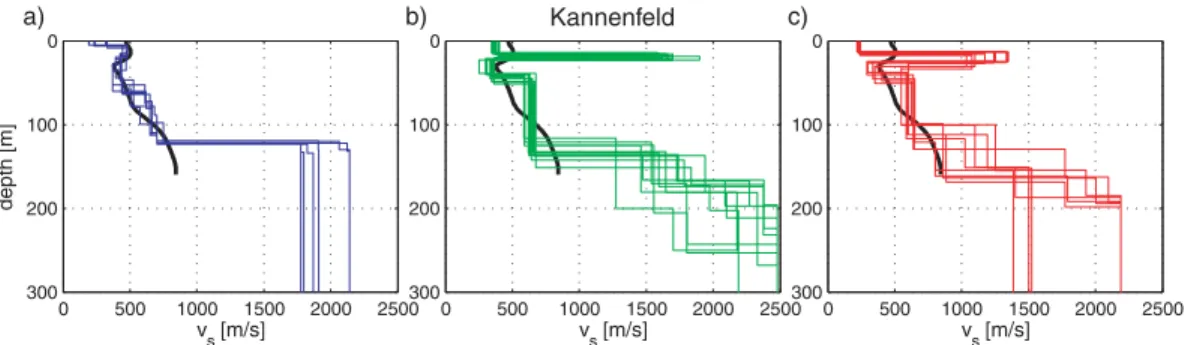
Results obtained from surface wave analysis and from reflection seismics (black) are shown in Fig. 16. Different inversions were per-formed: the first using the information from the vertical component and H/V ratios only (Fig. 16a); the second also using data from hor-izontal components (Figs 16b and c). For the inversion the allowed number of layers with soft sediments varied between 4 and 7. Agree-ment between the models is good. However, the dispersion curves of the Love waves cannot be explained with the models produced by analysing the vertical components (Fig. 17b1). This becomes clear when we compare the resulting structures from the combined inver-sion of phase velocity curves from Love and Rayleigh waves and ellipiticies of the fundamental mode Rayleigh wave with previous models (green and red structures in Fig. 16). All structures require a thin high-velocity layer at shallow depth, with thickness between 5 and 10 m and S-wave velocities in the range of 1100–1900 m s−1. We analysed the case in which the Rayleigh wave dispersion curve segment between 8 and 14 Hz is related to the fundamental mode (green structures) and the case where this segment corresponds to the first higher mode (red structures). Both hypotheses require this high velocity layer at shallow depth and thus indicate that the

grav-els must be strongly cemented. However, even if we consider the strong cementing, the values of this layer produced by the green models (above 1500 m s−1) are unrealistically high. In this regard the red models seem more reliable (values of the layer are less than 1400 m s−1). From this we may infer that the second branch is likely to be part of the first higher mode (assumption used for producing the red models).

One might expect a second peak in the H/V spectral ratio due to this strong velocity contrast. However, the high velocity layer at shallow depth is not thick enough to produce a contrasting layer for the wavelength under consideration. Waves with wavelength of about four times the thickness of the low-velocity surface layer do not see the thin high-velocity layer. At higher frequency we can expect the efficient trapping of seismic waves in the low-velocity surface layer. However, the effect on the H/V ratio is unknown. The high-velocity layer might also act as a shield for high-frequency incident waves from below.

This high-velocity stratum influences the phase velocity curves of Love waves, but has less impact on the curves for Rayleigh waves. Identifying this layer was, therefore, possible only by using Love wave data.

5 C O N C L U S I O N S

Ambient vibration array measurements are an efficient tool to obtain information on local structure. In addition to the classical analysis of the vertical component, this paper also presented results derived from processing horizontal components. We used fundamental and higher modes of Rayleigh and Love waves phase velocity curves as well as the ellipticity of the fundamental mode Rayleigh wave. This combination has advantages when compared to analyses of only ver-tical components and Rayleigh waves. The scatter is reduced and the velocity of the bedrock layer and the thickness of soft sediments can be better resolved. With the joint use of Rayleigh and Love wave information, some structures can also be excluded. Introducing ad-ditional geological or borehole information will also help improve inversion results by reducing the number of layers or constraining layer thickness. Reducing the number of soft-sediment layers dur-ing the inversion process with a genetic algorithm leads to a class of models that are less smooth with large velocity contrasts between layers. When performing an array analysis, we do not know the true model and cannot decide whether layer reduction is required.

0 2 4 6 8 10 5 0 0.5 1 log(H/V) Frequency [Hz] Kannenfeld: central station a) 0 2 4 6 8 10 0.5 0 0.5 1 log(H/V) Frequency [Hz] Kannenfeld b)

Figure 14. (a) H/V spectral ratios obtained for the central station for array at Kannenfeld. The black line is the result of the classical polarization analysis in

the frequency domain. It was corrected for SH waves using the assumption of equal amplitude of SH and P-SV waves on the horizontal components. The grey line was obtained with the method based on the frequency-time analysis. (b) Comparison of the H/V spectral ratios of all stations in the array using the classical polarization analysis.

0 5 10 15 0 500 1000 1500 2000 vertical ( • ), radial ( + ) frequency [Hz] c [m/s] subarray 1 subarray 2 subarray 3 subarray 4 a) 0 5 10 15 0 500 1000 1500 2000 transverse ( ♦ ) frequency [Hz] c [m/s] subarray 1 subarray 2 subarray 3 subarray 4 b) 0 5 10 15 0 500 1000 1500 2000 frequency [Hz] c [m/s] c) 0 1 0 5 10 15 0 500 1000 1500 2000 frequency [Hz] c [m/s] d) 0 1

Figure 15. Measured dispersion curves for Rayleigh (a, c) and Love waves (b, d). Vertical: analysis of the vertical components; radial: analysis of the radial

components; transverse: analysis of the transverse components. kminand kmax/2 of the subarrays are given, respectively, as dashed and dash-dotted lines and define the resolution limit of the subarray geometries. (a) and (b) Manually picked dispersion curves. (c) and (d) Segments used for the inversion (red).

0 500 1000 1500 2000 2500 0 100 200 300 v_s [m/s] depth [m] a) 0 500 1000 1500 2000 2500 0 100 200 300 v_s [m/s] Kannenfeld b) 0 500 1000 1500 2000 2500 0 100 200 300 v_s [m/s] c)

Figure 16. Inverted models from the array measurements (colour) compared to the results from seismic reflection (black, by Polom et al. 2005). (a) The blue

structures correspond to inversion using the Rayleigh wave phase velocity curves and ellipticity. (b) The green curves represent structures obtained when also using Love wave dispersion-curves, by assuming that the second segment (1 in Fig. 15c) of the measured Rayleigh wave dispersion-curve is related to the fundamental mode. The first segment (0 in Fig. 15c) is always related to the fundamental mode. The first segment of the Love wave dispersion-curve (0 in Fig. 15d) is related to the fundamental mode, the second segment (1 in Fig. 15d) to the first higher mode. (c) The same as (b) but assuming that the second segment of the measured Rayleigh wave dispersion-curve (1 in Fig. 15c) is related to the first higher mode.

However, by varying the number of layers in the inversion process, we can assess possible solutions between the extremes of smooth models and models with strong velocity contrasts. If two models with a different number of layers explain the measured data equally well with a similar misfit then the model with fewer layers should be chosen unless this model is geologically/geophysically unrealistic, or additional geological information is available that puts a strong preference on the model with extra layers. Using more geophysical layers than lithological units may be justified by the presence of a ve-locity gradient within the same unit. Havenith et al. (2007) resolved a velocity gradient within the gravel layers in our investigation area.

The increase of the velocity with depth is due to compaction of the material. Weathering of a lithological unit might cause a reduction of the velocity in its upper part. An example is the Meletta layer present at the site Kannenfeld.

For real sites, considerable variability in the measured phase ve-locity curves is introduced due to lateral changes of the structure or seismic sources within the array. Such sources can be of an-thropogenic origin or related to structural features or buildings that scatter the incident ambient vibration wavefield. Constraining the inversion through Love and Rayleigh wave information can help re-duce such problems. Frequency bands in which the Rayleigh wave

0 5 10 15 0 500 1000 1500 2000 Frequency [Hz] Phase v elocity [m/s ] a1) 0 5 10 15 0 500 1000 1500 2000 Frequency [Hz] Kannenfeld: Rayleigh a2) 0 5 10 15 0 500 1000 1500 2000 Frequency [Hz] a3) 0 5 10 15 0 500 1000 1500 2000 Frequency [Hz] Phase v elocity [m/s ] b1) 0 5 10 15 0 500 1000 1500 2000 Frequency [Hz] Kannenfeld: Love b2) 0 5 10 15 0 500 1000 1500 2000 Frequency [Hz] b3) 0 2 4 6 8 10 0 1 2 Frequency [Hz] Ellipticity c1) 0 2 4 6 8 10 2 1 0 1 2 Frequency [Hz] Kannenfeld: Ellipticity c2) 0 2 4 6 8 10 2 1 0 1 2 Frequency [Hz] c3)

Figure 17. (a, b) Comparison between dispersion curves of the inverted structural models and the observed curves (black) for Rayleigh (a) and Love waves (b).

(a1, b1) The blue dispersion curves were obtained using Rayleigh wave dispersion-curve segments and the ellipticity for the inversion. (a2, b2) The green/brown curves show the resulting dispersion curves when data from the Love waves are included in the inversion (green: fundamental mode; brown: first higher mode). We assume that the second segment (1 in Fig. 15c) of the measured Rayleigh wave dispersion-curve is related to the fundamental mode. (a3, b3) The same as (a2, b2) (red: fundamental mode; magenta: first higher mode) but assuming that the second segment of the measured Rayleigh wave dispersion-curve (1 in Fig. 15c) is related to the first higher mode. (c) Comparison between ellipticities of the fundamental mode Rayleigh wave and the H/V ratios computed for the central station of the array. The end-points of the segments used for the inversions are shown by arrows.

dispersion curves show considerable scatter are often better resolved by Love waves. Analysing radial components can also provide seg-ments of Rayleigh wave dispersion curves for modes not seen on the vertical component. Finally, with respect to Rayleigh waves, Love waves dispersion curves of different modes should be separated bet-ter from each other to make it easier to assign a mode number to the different Love wave phase-velocity curve segments. As a result, the ambiguity of resulting models is considerably reduced. The com-bined use of vertical and horizontal components especially allows better characterization of structures with strong velocity inversions. The example of the Kannenfeld site shows that a velocity inver-sion can influence the phase velocity curves of Love waves, but the curves of Rayleigh waves less so. This velocity inversion is correctly identified only by including the Love wave data.

Generally, bedrock S-wave velocity cannot be resolved due to the limited size of the arrays. Future studies should envisage addi-tional, larger arrays to resolve as well the dispersion curve segments with phase velocities as high as 2000–3000 m s−1. Such arrays would better constrain velocity values in deeper sediments and at

the sediment-bedrock interface. The velocity contrast between sedi-ments and bedrock and the bedrock velocity are essential parameters when site-amplification factors have to be estimated for local seis-mic hazard studies.

We conclude that ambient vibration techniques are still not used to their full potential, but progress is expected. In particular, we need more efficient numerical tools to retrieve ellipticity curves from H/V spectral ratios. To better constrain solutions and limit uncertainties related to measurements, we suggest the combined use of three-component ambient noise data, geological and geotechnical information, and passive as well as active geophysical techniques.

A C K N O W L E D G M E N T S

This research was enabled by a series of projects and research con-tracts: project SHAKE-VAL, funded by the Swiss National Science Foundation (No. 200021–101920 and 200020–109177), the Inter-reg project ‘Seismische Mikrozonierung am s¨udlichen Oberrhein’,

and the European project ‘Site effects assessment using ambient excitations’ SESAME, funded for Swiss participants by the Swiss Federal Office for Education and Science (BBW No. 00.0085-2). We thank G.F. Panza and the Seismology Group of Trieste Univer-sity for the use of the spectral part of the Rayleigh waves program. We would like to thank our reviewers for helping to improve this work and our English editor, Dr Kathleen J. Jackson.

R E F E R E N C E S

Bard, P.-Y., 1998. Microtremor measurements: a tool for site effect estima-tion?, Proceeding of the Second International Symposium on the Effects of Surface Geology on Seismic Motion, Yokohama, Japan, Vol. 3, pp. 1251–1279.

Bonnefoy-Claudet, S., Cotton, F., & Bard, P.-Y., 2006a. The nature of noise wavefield and its applications for site effects studies. A literature review. Earth-Sci. Rev., 79, 205–227.

Bonnefoy-Claudet, S., Cornou, C., Bard, P.-Y., Cotton, F., Moczo, P., Kristek, J. & F¨ah, D., 2006b. H/V ratio: a tool for site effects evaluation. Results from 1D noise simulations, Geophys. J. Int., 167, 827–837.

Capon, J., 1969. High-resolution frequency-wave number spectrum analysis, Proc. IEEE, 57(8), 1408–1418.

F¨ah, D., Kind, F. & Giardini, D., 2001. A theoretical investigation of average H/V ratios, Geophys. J. Int., 145, 535–549.

F¨ah, D., Kind, F. & Giardini, D., 2003. Inversion of local S-wave velocity structures from average H/V ratios, and their use for the estimation of site-effects, J. Seismol., 7, 449–467.

Florsch, N., F¨ah, D., Suhadolc, P. & Panza, G.F., 1991. Complete synthetic seismograms for high frequency multimode SH-waves, Pageoph, 136, 529–560.

Havenith, H.B., F¨ah, D., Pollom, U. & Roulle, A., 2007. S-wave velocity measurements applied to the seismic microzonation of Basel, Upper Rhine Graben, Geophys. J. Int., 170, 346–358.

Hisada, Y., 1994. An efficient method for computing Green’s functions for a layered half-space with sources and receivers at close depths, Bull. seism. Soc. Am., 84(5), 1456–1472.

Hisada, Y., 1995. An efficient method for computing Green’s functions for a layered half-space with sources and receivers at close depths (Part 2), Bull. Seism. Soc. Am., 85(4), 1080–1093.

Kind, F., 2002. Development of Microzonation Methods: Application to Basle, Switzerland, PhD thesis, No.14548, Swiss Federal Institute of Tech-nology, Zurich.

Kind, F., F¨ah, D. & Giardini, D., 2005. Array measurements of S-wave velocities from ambient vibrations, Geophys. J. Int., 160, 114–126. Nakamura, Y., 1989. A method for dynamic characteristics estimation of

subsurface using microtremor on the ground surface, QR of RTRI, 30, 25–33.

Ohrnberger, M., 2004. User manual for software package CAP—a continu-ous array processing toolkit for ambient vibration array analysis, SESAME report D18.06, pp. 83 (http://sesamefp5.obs.ujf-grenoble.fr).

Panza, G.F., 1985. Synthetic seismograms: the Rayleigh waves modal sum-mation, J. Geophys., 58, 125–145.

Panza, G.F. & Suhadolc, P., 1987. Complete strong motion synthetics, in Seismic Strong Motion Synthetics, Vol. 4 Computational Techniques, pp. 153–204, ed. Bolt, B.A., Academic Press, London.

Parolai, S., Richwalski, S.M., Milkereit, C. & F¨ah, D., 2006. S-wave ve-locity profiles for earthquake engineering purposes for the Cologne Area (Germany), Bull. Earthq. Eng., 4, 65–94.

Polom, U., F¨ah, D., Havenith, H.-B., Pohl, C., Roull´e, A., Stange, S. & Steiner, B., 2005. Shear wave velocity-depth determination for the upper Rhine mid/south seismic risk microzonation, Proceedings of the EAGE Near Surface 2005 Conference & Exhibition, 04.-07.09.2005, Palermo, Italy.

Roten, D. & F¨ah, D., 2007. A combined inversion of Rayleigh wave dispersion and 2-D resonance frequencies, Geophys. J. Int., 168, 1261–1275.

Roten, D., F¨ah, D., Cornou, C. & Giardini, D., 2006. Two-dimensional res-onances in Alpine valleys identified from ambient vibration wavefields, Geophys. J. Int., 165, 889–905.

Satoh, T., Kawase, H., Iwata, T., Higaski, S., Sato, T., Irikura, K. & Huang, H.C., 2001. S-wave velocity structure of Taichung basin, Taiwan estimated from array and single-station records of microtremors, Bull. seism. Soc. Am., 91, 1267–1282.

SESAME Deliverable D12.09, 2004. Report on Simulation of seismic noise (WP09): report on parameter studies Site Effects Assessment Using Am-bient Excitations, European Commission – Research General Directorate, Project No. EVG1-CT-2000–00026 SESAME. December 2004. Steimen, S., F¨ah, D., Kind, F., Schmid, C. & Giardini, D., 2003. Identifying

2-D resonance in microtremor wave fields, Bull. seism. Soc. Am., 93, 583–599.

Tokimatsu, K., 1997. Geotechnical Site Characterization using Surface Geotechnical Engineering, pp. 1333–1368, AA Balkema, Rotterdam. Wathelet, M., 2005. Array Recordings of Ambient Vibrations: Surface-Wave

Inversion, p. 177, Li`ege University, Belgium.

Yamanaka, H., Takemura, M., Ishida, H. & Niea, M., 1994. Characteristics of long-period microtremors and their applicability in exploration of deep layers, Bull. seism. Soc. Am., 84, 1831–1841.