HAL Id: inserm-00855392
https://www.hal.inserm.fr/inserm-00855392
Submitted on 26 Aug 2014HAL is a multi-disciplinary open access archive for the deposit and dissemination of sci-entific research documents, whether they are pub-lished or not. The documents may come from teaching and research institutions in France or abroad, or from public or private research centers.
L’archive ouverte pluridisciplinaire HAL, est destinée au dépôt et à la diffusion de documents scientifiques de niveau recherche, publiés ou non, émanant des établissements d’enseignement et de recherche français ou étrangers, des laboratoires publics ou privés.
A new deconvolution approach to robust fluence for
intensity modulation under geometrical uncertainty.
Pengcheng Zhang, Renaud de Crevoisier, Antoine Simon, Pascal Haigron,
Jean-Louis Coatrieux, Baosheng Li, Huazhong Shu
To cite this version:
Pengcheng Zhang, Renaud de Crevoisier, Antoine Simon, Pascal Haigron, Jean-Louis Coatrieux, et al.. A new deconvolution approach to robust fluence for intensity modulation under geometrical uncer-tainty.. Physics in Medicine and Biology, IOP Publishing, 2013, 58 (17), pp.6095-110. �10.1088/0031-9155/58/17/6095�. �inserm-00855392�
A new deconvolution approach to robust fluence for
intensity modulation under geometrical uncertainty
Pengcheng Zhang1, 2, 3, 4, Renaud De Crevoisier2, 3, 4, Antoine Simon2, 3, 4,
Pascal Haigron2, 3, 4, Jean-Louis Coatrieux1,2, 3, 4,!Baosheng Li5, and
Huazhong Shu1, 4
1Laboratory of Image Science and Technology, Southeast University, Nanjing 210096, China
2INSERM, U1099, Rennes 35042, France
3Laboratoire Traitement du Signal et de l’Image, Universite de Rennes I, Rennes 35042 France
4Centre de Recherche en Information Médicale Sino-français (CRIBs) 5Shandong Tumor Hospital, Jinan 250117, China
Email: [email protected]
Abstract. This work addresses random geometrical uncertainties that are intrinsically observed in radiation therapy by means of a new deconvolution method combining a series expansion and a Butterworth filter. The method efficiently suppresses high frequency components by discarding the higher order terms of the series expansion and then filtering out deviations on the field edges. An additional approximation is made in order to set the fluence values outside the field to zero in the robust profiles. This method is compared to the deconvolution kernel method for a regular 2D fluence map, a real intensity-modulated radiation therapy (IMRT) field, and a prostate case. The results show that accuracy is improved while fulfilling clinical planning requirements.
1. Introduction
Sources of geometrical uncertainty that hamper exact delivery of a plan may include patient set-up variation (i.e., repositioning), organ motion and deformation, as well as machine-related errors (Stroom et al 2002). Systematic uncertainties can be reduced using image-guidance techniques and adaptive radiotherapy (Yan et al 1998, Hoogeman et al 2005, de la Zerda et al 2007, Peng et al 2011). Large organ movements, such as those observed in lung or prostate cancers (Suh et al 2009), can be compensated for using real-time motion tracking. However, random uncertainties cannot be fully eliminated (Fan and Nath 2010), due
to the finite response time and irregular motion patterns (Webb 2006).
Conventional methods of adding a margin around the clinical target volume (CTV) so as to obtain a planning target volume (PTV) aim to find a sound compromise between maximizing target dose and minimizing dose to OAR, i.e., organ at risk (Baum et al 2006). Several methods have been proposed to account for geometric uncertainties in dose calculation, such as the “stochastic simulation method” (Lujan et al 1999), the “dose convolution method” (McCarter and Beckham 2000, Craig et al 2003), and the “fluence modification method” (Lu et al 2005). However, these methods inevitably expand CTV area. To significantly reduce the PTV margin, other authors (Lind et al 1993, Lof et al 1995, Gordon and Siebers 2008, Bortfeld et al 2008, Moore et al 2009, Fan and Nath 2010) have used the “robust beam profile” method, of which the most important feature is the higher fluence delivered on the field edges.
In this work, we concentrated our attention on random geometrical uncertainties. Various deconvolution algorithms have been investigated in order to calculate robust beam profile with respect to small random geometrical uncertainties (Lind et al 1993, Fan and Nath 2010), and to remove the finite detector size effect in the measured profiles (Ulmer and Kaisel 2003, Ulmer 2010). To avoid infeasible or unreliable deconvolution results using the direct inverse filtering in the frequency domain, the series expansion method has been employed for first-order approximation of the deconvolution (Fang et al 1994, Garcia-Vicente et al 2000, Ulmer and Kaissl 2003, Fan and Nath 2010, Ulmer 2010). High-frequency components were suppressed through the summation of the first four terms of series expansion. The series expansion method can effectively suppress the oscillations in deconvolution results, but the effect is limited, and the convolved-back results inevitably contain numerous high frequency components, especially around the field edges. The method proposed by Fan and Nath (2010) is one kind of series expansion method that suppresses the fluence around the field edges. If the suppression is too large, however, it could lead to inferior intensity in the convolved-back profiles than in the nominal static fluence map around the field edges. Here we proposed a new deconvolution method based on series expansion and a Butterworth filter. In order to suppress the high-frequency components, we used only the first four terms of the series. By adjusting the parameters of the Butterworth filter according to the different probability density functions (PDF), we further suppressed high-frequency signal components and minimized differences between the static and convolved-back profiles, especially on the field edges.
This paper is organized as follows: First, the methods and principles used in the design of the algorithm are described. Then, the new deconvolution approach is detailed (Section 2). The results are presented in Section 3, including a comparison to the deconvolution kernel method for a regular 2D fluence map and a real IMRT field. We also tested the proposed technique on a prostate case, the results of which are discussed in Section 4 prior to the conclusion.
2. Methods
Geometrical uncertainty results from many independent random causes (setup variation, motion, equipment precision limit, etc.), as discussed above. According to the central limit theorem, the distribution of this uncertainty should converge to the Gaussian distribution in a
multi-fraction treatment (Fan and Nath 2010).We used a single Gaussian distribution to describe random patient motion, as reported before on robust fluence (Unkelbach and Oelfke 2005, Chu et al 2005, Moore et al 2009, Fan and Nath 2010):
2 2
1
( , )
exp
.
2
2
x
p
!
x
!
"!
#
$
=
&
%
'
(
)
(1) Here, the standard derivation ! describes the random motion. Given a beam profile, the convolved-back profile Dm(x) is defined as:Dm(x)=
!
p(#
,x"u)Dp(u)du, (2) where Dp(u) is the deconvolution profile. Our goal was to obtain the optimal deconvolutionfluence map Dp(u) by minimizing the differences between the convolution-back fluence map
Dm(x) and the nominal static fluence map.
2.1. The beam profile deconvolution with the series expansion method
With the Taylor serial expansion of Dp(u) at x, equation (2) can be written as:
Dm(x)=ADp(x), (3) where the operator is
2 (2) 2 (2 ) 2 2 0 1 exp . 2 ! 2 n n n n d d A n dx dx ! " ! = # $ # $
= %% &&= %% &&
' (
)
' (The inverse operator A-1, defined by Ulmer and Kaissl (2003), leads us to formulate the deconvolution from Dm to Dp as:
1 2 (2) 2 ( ) ( ) exp ( ) 2 p x A m x d m x dx ! " # $ = = %%" && ' ( D D D . (4)
Ulmer and Kaissl alsoderived an expression of the inverse PDF or deconvolution kernel
p-1(!, x), which allows the deconvolution to be calculated in the following integral form: Dp(x)=
!
p"1(#
,x"u)Dm(u)du. (5) In equation (5), the representation of p-1(!, x) can be expressed in the expansion of Hermite polynomials H2n: 1 2 0 ( , ) ( , ) 2 n n n x p ! x c H p ! x ! " # = $ % = & ' ( )*
, (6)with the coefficients cn=(–1)n/(2nn!).
2.2. 1D beam profile deconvolution
The Fourier transform of equation (4) can be expressed in the following form:
2 1 2 0 1 { ( )} { ( )} ! 2 n n m m n F A u w F u n ! " # = $ % = && '' ( )
*
D D (7)where w is the angular frequency. Following Ulmer and Kaissl (2003), the deconvolution kernel p-1(!, x) can also be written as:
p"1( , )! x =A p"2 ( , )! x , (8) where 2 2 (2)2 2 (2 )2 0 1 exp ( 1) ! n n n n n d d A n dx dx ! " ! # = $ % = &&# ''= #
( )
*
. Then, the Fourier transform of thedeconvolution kernel p-1(!, x) is exp( /2) ! 1 )} , ( { 2 2 2 2 0 1 ! ! w w ! n x p F n n n " =
#
$ = " . (9)Using the Fourier transform to equation (5), we obtain
exp( /2) { ( )} ! 1 )} ( { 2 2 2 2 0n w w F u x F n n m n p D D =
#
$ ! " ! = . (10) By comparing equation (7) with equation (10), a filter H(w) can be defined as:)} ( { ) ( } ) ( ) , ( { p 1 x u u du H w F A 1 u F
"
!#
! Dm = !Dm , (11) where 2 2 2 2 0 2 2 0 1 ! ( ) exp( / 2) 1 ! 2 n n n n n n w n H w w w n ! ! ! " = " = = # $ % & ' & ' ( )*
*
. (12)Note that H(w) = 1 corresponds to an all-pass filter through the summation of polynomials to infinity. Due to the small contributions of the higher order terms, we only consider the first four terms in the summation of equation (12). In this context, H(w) is a filter that suppresses part of the high-frequency components.
The convolved-back profiles for the deconvolution using the series expansion method in equation (4) and the deconvolution kernel method in equation (5) are shown in Figure 1, where the series expansion method is labeled as “Series” and the deconvolution kernel method is labeled as “DK”. We found that there are large deviations around the edges of fields between the convolved-back profiles and the static profile. However, the convolved-back profiles using the deconvolution kernel method are better than the results of the series expansion method, because the convolved-back profiles from the deconvolution kernel method are equal to the product of the results from the series expansion method and a low-pass filter. The frequency response of this low-pass filter is related to the truncation of the terms considered in equation (12). In order to further reduce the differences between the convolved-back profiles and the static profile, we filtered the results of the series expansion method with a classical filter whose frequency response could be more easily adjusted. To this end, we used a Butterworth filter with a frequency response of:
2 0 1 ( ) , 1 ( / ) m H w w w = + (13)
where w0 is the cutoff frequency and m is the number of reactive elements (poles) in the filter. In the series expansion (equation (7)) we just took the first four terms of the series--the low frequency components gathering most of the signals’ intensity. By adjusting the filter parameters, we could easily suppress the signals’ high-frequency components according to different PDF, and reduce differences between the static profile and the convolved-back profiles on the field edges, as shown in Figure 1, where the proposed method is labeled as “Filter.”
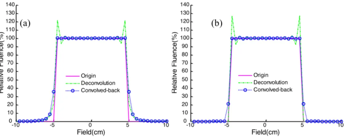
To reduce the dose delivered outside the field, a further approximation was made by setting the values of deconvolution profiles outside the field to zero (Figure 2). This may reduce the intensities of convolved-back profiles on the field edges, as no dose is received outside the field. Thus, it is necessary to readjust the filter parameters in order to compensate for these lower intensities by the increased dose received on the field edges, as shown in Figure 2(b). The parameters of the filter were set by systematically exploring the parameter space for the minimal difference between the convolved-back profile and the nominal static profile.
2.3. Extension to 2D fluence deconvolution
The 2D extension can be derived following the same approach. For a 2D Gaussian PDF:
2 2 2 2 1 ( , , , ) exp 2 2 2 x y x y x y x y p! ! x y "! ! ! ! # $ % & = %' ' & ( ) , (14) where the variables x and y are independent and separable; therefore, the extension of the 1D operator equation (3) to 2D is straightforward:
2 2 2 2 2 2 exp exp 2 2 y x d d A dx dy ! ! " " # # " " # # $ $ % % = $$&$$ %% %% $&$ % % ' ( ' ( ' ' ( ( . (15) The deconvolution procedure is similar; the corresponding Fourier transform in each dimension is written as:
2 2 2 2 0 0 1 1 { ( , )} { ( , )} ! 2 ! 2 k n y n k x p m n k F x y u v F x y n k ! ! " " = = # $ # $ % & = %% && % &
' ( ' (
)
)
D D , (16)
where u and v are the angular frequency. To reduce fluctuations within the field, the deconvolution outputs were filtered by a Butterworth filter in each dimension. We wrote the 2D Butterworth filter in the frequency domain as follows:
2 2 0 0 1 1 ( , ) , 1 ( / ) m 1 ( / ) k H u v u u v v = + + (17)
where u0 and v0 are the cutoff frequencies, and m and k are the number of reactive elements (poles) of the filter in each dimension.
In this work, the proposed method was compared to the improved deconvolution kernel method given by Fan and Nath (2010). That method achieves the deconvolution kernel by taking the first four Hermite polynomials in equation (6) in the Cartesian coordinate system and then effectuating an approximate conversion to the polar coordination system through a triangular transformation.Fan’s method suppresses the fluence around the field edges. If the
suppression is too large, however, it may lead to lower intensity in the convolved-back profiles than in the static fluence map around the field edges, as shown in Figure 3.
3. Results
We simulated two kinds of intensity-modulated 2D fluence maps, as shown in Figure 4(a) and Figure 5(a), and tested our method on a prostate case (Figure 7(a)). The patient PDF is the PDF modelling random geometric uncertainties of patient in 3D space. In this work, the PDF
p(!x, !y, x, y) is a projection of the patient PDF to a plane orthogonal to the beam direction.
Standard deviations of !x = 4 mm and !y = 3 mm were chosen for 2D PDF in x- and y-
directions, respectively (in equation (14)). These standard deviations are the typical random geometrical uncertainty in practice for various sites (van Herk et al 2002, Moore et al 2009). To obtain a high cutoff frequency and a low order for the Butterworth filter, as discussed above, we used the parameters u0 = 0.9375, n = 1 and v0 = 1.25, k = 1 in equation (17), respectively, for these two standard deviations. Note that the values of cut-off frequencies u0 and v0 were selected by an exhaustive search in order to minimize the difference between the convolved-back fluence map and the static fluence map. The same filter parameters were employed for different fluence maps with equal standard deviations. Three different methods (“DK”--the deconvolution kernel method (Ulmer and Kaissl 2003), “IDK”--the improved deconvolution kernel method (Fan and Nath 2010), and “Filter”--the proposed method) were compared, both for the two kinds of fluence maps and the prostate case.
We calculated dose distribution as follows:
(i) The deconvolution fluence maps were obtained via the deconvolution methods mentioned above;
(ii) We sequenced the deconvolution fluence map into a series of deliverable leaf sequences, and then reconstructed these deliverable leaf sequences into a deliverable fluence map;
(iii) The convolved-back fluence map was then calculated by convolving the deliverable fluence map and equation (14);
(iv) Finally, the convolved-back fluence map was inserted into the software CERR (Deasy et al 2003), in order to calculate the dose distribution.
3.1. Results for a regular 2D fluence map
Figure 4 shows the application of the 2D deconvolution algorithms to the regular 2D fluence map. Ideally, the convolved-back fluence maps (Figure 4(b), (c) and (d)) should be the same as the nominal static one (Figure 4(a)). The differences between the convolved-back fluence maps and the static fluence map lie mainly around the field edges due to the nominal static fluence map’s steep fall-off. A detailed comparison of convolved-back fluence maps is also shown in a profile plot in Figure 4(e) for these three methods.
As shown in Figure 4, the convolved-back fluence map based on the proposed method exhibits fewer hot or cold spots than the results with the other two methods. Much improved agreement on fluence distributions around the field edges was achieved. The difference between the nominal static fluence map and the convolved-back fluence map was measured by the quadratic sum defined as:
d =
""
(
F
ori!
F
con) ,
2 (18) where Fori is the nominal static fluence distributions and Fcon is the convolved-back fluencedistributions. For this regular 2D fluence map, the quadratic sums of the difference between the nominal static map and the convolved-back fluence maps in the field were 0.7070, 0.4680, and 0.0577, for the deconvolution kernel method, the improved deconvolution kernel method, and the proposed method, respectively.
3.2. Results for an IMRT field
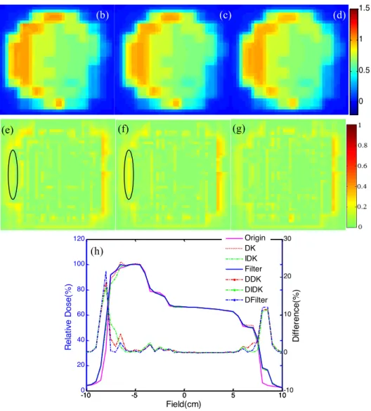
Figure 5 shows the application of the 2D deconvolution algorithms to the fluence map of an IMRT field. Compared to the nominal static fluence map (Figure 5(a)), the deconvolution fluence maps (Figure 5(b)-(d)) displayed a higher intensity on the field edges, especially in the lateral direction (x-direction), due to a larger random geometrical uncertainty and the steeper intensity edges. The convolved-back fluence maps and the corresponding differences to the nominal static fluence map are depicted in Figure 5(e)-(g) and 5(h)-(j). A profile comparison of the convolved-back fluence maps is shown in Figure 5(k).
The deconvolution fluence map (Figure 5(d)) computed using the proposed method is less smooth than those calculated using the other two methods (Figure 5(b)-(c)). However, the convolved-back fluence map (Figure 5(g)) is closer to the static fluence map than the two corresponding convolved-back fluence maps (Figure 5(e)-(f)), especially on the field edges, as shown in Figure 5(h)-(j). For the deconvolution kernel method, the improved deconvolution kernel method, and the proposed method, the quadratic sums of the difference between the nominal static fluence map and the convolved-back fluence maps were 1.2014, 1.0460, and 0.6884, respectively, in the field. As depicted in Figure 5, the proposed method achieved superior agreement on fluence distributions around the field edges.
We input the convolved-back fluence maps (Figure 5) into the software CERR (Deasy et
al 2003) in order to calculate the dose distribution for a 6 MV photon beam at 10 cm depth of
a water phantom, and the corresponding results are shown in Figure 6, where Figure 6(a)-(d) displays the dose distribution from the static fluence map in Figure 5(a) and from the convolved-back fluence maps in Figure 5(e)-(g). We used the gamma evaluation method (Low et al 1998) in order to analyze the dose distribution calculated from convolved-back fluence maps. The gamma analysis was applied with a dose difference of 3% and a distance to agreement of 3 mm. The 2D gamma analysis is shown in Figure 6(e)-(g), and the dose profiles are shown in Figure 6(h). We observed that the dose distributions calculated using the proposed method were closer to the dose distribution calculated from the nominal static fluence map than those calculated using the other two methods, especially around the field edges.
3.3. Results for a prostate case
Our method was tested on a prostate case with one 6 MV photon beam extracted from a 5-beam IMRT plan. The gantry angle was 900, and the beam’s source-axis distance was 100 cm. Figure 7 displays one slice of the CT scans, along with the static fluence map we used. The sensitive normal tissues considered here were the rectum wall and bladder wall (Figure
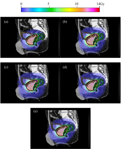
7(a)). We calculated dose distributions for both the nominal static fluence map and the fluence maps obtained using the margin expansion and deconvolution methods. The margin expansion method enlarged the static fluence map by 0.5 mm in each direction. Figure 8 shows the 2D dose distributions at 17 cm under the surface in the beam direction for those fluence maps. We observed that high doses were partially delivered to the region outside the CTV when this approach was used (Figure 8(b)). When the deconvolution kernel method was applied, the delivered dose was high around the target edges (Figure 8(c)). The improved deconvolution kernel method (Figure 8(d)) and the proposed method (Figure 8(e)) showed a better dose modulation than the margin expansion method. Dose volume histograms (DVH) for the 2D dose distributions (Figure 8) are displayed in Figure 9. For the sensitive normal tissues, the proposed method offered better control for high doses delivered to normal tissue than the other three methods (Figure 9(a) and (b)). For the CTV, the dose distributions obtained using the proposed method were closer to the nominal static fluence map than those resulting from the other three methods (Figure 9(c)). We also analyzed the 2D dose distributions for the deconvolution method with gamma evaluation. A significant reduction of the difference in dose distributions was achieved with the proposed method, as shown in Figure 10.
We used the method proposed by Engel (2005) in order to sequence the fluence map into a deliverable leaf sequence. In this work, the pixel size in fluence map was 0.5!0.5 cm2, and the minimum monitor unit (MU) was 5 MU for each segment. Thus, the resulting fluence maps were deliverable. With 10, 17, 14, and 16 segments, the fluence map monitor units equaled 85, 275, 175, and 210 for the margin expansion method, the deconvolution kernel method, the improved deconvolution kernel method, and the proposed method, respectively. 4. Discussion and conclusion
This study’s main assumption was that the organ motions of interest are random, with known probability distributions. Under this hypothesis, several works based on the deconvolution algorithm have been reported in the literature to derive a robust fluence map for IMRT. The advantages and disadvantages of this kind of approaches have been discussed by Fan and Nath. They showed that the deconvolution approach is more suitable for IMRT fluences with random geometrical uncertainties with a standard deviation within 2 and 4 mm, which means that the motion uncertainty is not very high. In this context, we have proposed a new deconvolution approach for robust fluence.
Our proposed solution combines series expansion and filtering techniques. We now have access to optimal filters, the choice among which (Bessel, Chebyshev, elliptic, etc.) depends on several features, such as the behavior in pass-band, roll-off factor (this factor determines the vertical extent of the transition zone between the pass-band and stop-band), phase response, and execution speed. Bessel filters, for instance, transition more sharply between pass-band and stop-band, but do not provide the best phase response. The Butterworth filter selected here provides the flattest pass-band and a low roll-off factor. The main objective was, first, to show some of the benefits of the proposed combination. The use of other filters will be further explored in the future.
In addition, the proposed method offers the advantage that the whole formulation described operates in the frequency domain instead of the spatial domain. The Butterworth
filter can filter out the deviations around the field edges directly in the frequency domain. The parameters of the 2D Butterworth filter can be determined in each direction due to the independence and separability of arguments of PDF in the x- and y-directions. Their setting, varying with the PDF standard deviation, was designed to seek the minimum difference between the convolved-back fluence map and the static fluence map. It may be improved by replacing the exhaustive search with an optimization procedure.
Comparisons with two other deconvolution approaches (Ulmer and Kaissl 2003, Fan and Nath 2010) show that the difference between the nominal static fluence map and the convolved-back fluence map, as measured by the quadratic sum, is significantly reduced with the proposed method. This advantage is somehow less pronounced when real IMRT data are processed.
The convolved-back fluence map presents the actual fluence delivered to a patient when motion is accounted for. Our goal was to cause the target to receive the same fluence during motion as the nominal static fluence map; namely, to reduce the deviations between the static fluence map and convolution-back fluence map. Usually, there are large gradients in the static fluence map. The proposed method increases TNMU complexity (i.e., total number of monitor units) in the deconvolution fluence map, as defined by Engel (2005). For the prostate case reported in this work, these complexities were 83.62MU, 268.05MU, 179.26MU, and 206.59MU for the margin expansion, deconvolution kernel, improved deconvolution kernel, and proposed method, respectively.
To conclude, this new approach using both series expansion and a Butterworth filter was tested on two 2D fluence maps and a prostate case. It was shown that the Butterworth filter better suppressed high-frequency oscillations and reduced hot and cold spots on convolved-back fluence profiles. Better oscillation suppression could be obtained using the filter on different decomposed frequency bands as recently proposed by Yang et al (2012). In the flat area of the fluence map, our method’s accuracy was similar to that of the deconvolution kernel method. Near the edge of the fluence map, a clear advantage was observed. This approach can be easily implemented in the clinical setting and thus improve dose homogeneity.
Acknowledgments
This work was supported by the National Basic Research Program of China under Grant 2011CB707904, by the National Natural Science Foundation of China under Grants 61073138, 61271312, 61201344, and 60911130370, by the Ministry of Education of China under Grants 20110092110023, by the Key Laboratory of Computer Network and Information Integration (Southeast University), Ministry of Education, and by the Centre de
Recherche en Information Médicale Sino-français (CRIBs).
References
Baum C, Alber M, Birkner M and Nusslin F 2006 Robust treatment planning for intensity modulated radiotherapy of prostate cancer based on coverage probabilities Radiotherapy and Oncology 78 27-35
Bortfeld T, Chan T C Y, Trofimov A and Tsitsiklis J N 2008 Robust management of motion uncertainty in intensity-modulated radiation therapy Oper. Res. 56 1461-73
Chen Y, Yang Z, Hu Y, Yang G, Luo L, Chen W and Toumoulin C 2012 Thoracic low-dose CT image processing using an artifact-suppressed large-scale nonlocal means Phys. Med. Biol. 57 2667-88 Chu M, Zinchenko Y, Henderson S G and Sharpe M B 2005 Robust optimization for intensity
modulated radiation therapy treatment planning under uncertainty Phys. Med. Biol. 50 5463-77 Craig T, Battista J and Van Dyk J 2003 Limitations of a convolution method for modeling geometric
uncertainties in radiation therapy. I. The effect of shift invariance Med. Phys. 30 2001-11
de la Zerda A, Armbruster B and X Lei 2007 Formulating adaptive radiation therapy (ART) treatment planning into a closed-loop control framework Phys. Med. Biol. 52 4137-53
Deasy J O, Blanco A I, Clark V H 2003 CERR: a computational environment for radiotherapy research Med. Phys. 30 979-85.
Engel K 2005 A new algorithm for optimal multileaf collimator field segmentation Discrete Appl. Math 152 35-51
Fan Y and Nath R 2010 Intensity modulation under geometrical uncertainty: a deconvolution approach to robust fluence Phys. Med. Biol. 55 4029-45
Fang M T, Shei S S, Nagem R J and Sandri G v H 1994 Convolution and deconvolution with Gaussian kernel Nuovo Cimento B 109 83-92
Garcia-Vicente F, Delgado J M and Rodriguez C 2000 Exact analytical solution of the convolution integral equation for a general profile fitting function and Gaussian detector kernel Phys. Med. Biol. 45 645-50
Gordon J J and Siebers J V 2008 Evaluation of dosimetric margins inprostate IMRT treatment plans Med. Phys. 35 569-75
Hoogeman M S, van Herk M, de Bois J, and Lebesque J V 2005 Strategies to reduce the systematic error due to tumor and rectum motion in radiotherapy of prostate cancer Radiother. Oncol. 74 177-85
Lind B K, Kallman P, Sundelin B and Brahme A 1993 Optimal radiation beam profiles considering uncertainties in beam patient alignment Acta Oncol. 32 331-42
Lof J, Lind B K and Brahme A 1995 Optimal radiation beam profiles considering the stochastic process of patient positioning in fractionated radiation therapy Inverse Problems 111189-209 Low D A, Harms W B, Mutic S and Purdy J A 1998 A technique for the quantitative evaluation of dose
distributions Med. Phys. 25 656-61
Lu W, Olivera G H and Mackie T R 2005 Motion-encoded dose calculation through fluence/sonogram modification Med. Phys. 32 118-127
Lujan A E, Ten Haken R K, Larsen E W and Balter J M 1999 Quantization of setup uncertainties in 3-D dose calculations Med. Phys. 26 2397-402
McCarter S D and Beckham W A 2000 Evaluation of the validity of a convolution method for incorporating tumor movement and setup variations into the radiotherapy treatment plans, Phys. Med. Biol. 45 923-31
Moore J A, Gordon J J, Anscher M S and Siebers J V 2009 Comparisons of treatment optimization directly incorporating random patient uncertainty with a margin-based approach Med. Phys. 36 3880-90
Peng C, Chen G, Ahunbay E E, Wang D, Lawton C and Li X A 2011 Validation of an online replanning technique for prostate adaptive radiotherapy Phys. Med. Biol. 56 3659-68
Stroom J C, Heijmen B J 2002 Geometrical uncertainties, radiotherapy planning margins, and the ICRU-62 report Radiotherapy and Oncology 64 75-83
Suh Y, Sawant A, Venkat R and Keall P J 2009 Four-dimensional IMRT treatment planning using a DMLC motion tracking algorithm Phys. Med. Biol. 54 3821-35
Ulmer W 2010 Inverse problem of linear combinations of Gaussian convolution kernels (deconvolution) and some applications to proton/photon dosimetry and image processing Inverse Problems 26 1-26 Ulmer W and Kaissl W 2003 The inverse problem of a Gaussian convolution and its application to the
finite size of the measurement chambers/detectors in photon and proton dosimetry Phys. Med. Biol. 48 707-27
Unkelbach J and Oelfke U 2005 Incorporating organ movements in IMRT treatment planning for prostate cancer: minimizing uncertainties in the inverse planning process Med. Phys. 32 2471-83 van Herk M 2004 Errors and margins in radiotherapy Semin. Radiat. Oncol. 14 52-64
van Herk M, Remeijer P and Lebesque J V 2002 Inclusion of geometric uncertainties in treatment plane valuation Int. J. Radiat. Oncol. Biol. Phys. 52 1407-22
Webb S 2006 Quantification of the fluence error in the motion-compensated dynamic MLC (DMLC) technique for delivering intensity-modulated radiotherapy (IMRT) Phys. Med. Biol. 51 L17-21 Yan D, Ziaja E, Jaffray D, Wong J, Brabbins D, Vicini F, and Martinez A 1998 The use of adaptive
radiation therapy to reduce setup error: A prospective clinical study Int. J. Radiat. Oncol., Biol., Phys. 41 715-20
-10 -5 0 5 10 0 10 20 30 40 50 60 70 80 90 100 110 120 Field(cm) Rel at ive F luenc e( % ) Origin Series DK Filter -10 -5 0 5 10 0 10 20 30 40 50 60 70 80 90 100 110 120 130 140 Field(cm) Rel at ive F luenc e( % ) Origin Deconvolution Convolved-back -10 -5 0 5 10 0 10 20 30 40 50 60 70 80 90 100 110 120 130 140 Field(cm) Rel at ive F luenc e( % ) Origin Deconvolution Convolved-back -10 -5 0 5 10 0 10 20 30 40 50 60 70 80 90 100 110 120 Field(cm) Rel at ive F luenc e( % ) -10 -5 0 5 10 -10 0 10 20 30 40 50 Di ffer enc e( % ) Origin DK IDK Filter DDK DIDK DFilter
Figure 1. The profile for a static target and the correspondent convolved-back profiles for deconvolution profiles. “Origin”—nominal static profile, “Series”—profile obtained with the series expansion method in equation (4), “DK”—profile obtained with the deconvolution kernel method, “Filter”—profile obtained with the proposed method. A Gaussian distribution of geometrical uncertainty with standard deviation ! = 3 mm is assumed
Figure 3. The profiles for a static target and the corresponding convolved-back profiles. “Origin”— nominal static profile, “DK”—the deconvolution kernel method, “IDK”—the improved deconvolution kernel method, “Filter”—the proposed method. The dash-and-dot lines present the corresponding absolute difference with static profile and symbol prefix “D” for each method name. Gaussian Figure 2. A rectangle-field profile: “Origin”—nominal profile for a static target, “Deconvolution”— the
deconvolution profile, “Convolved-back”—the convolved-back profile. (a) The proposed method; (b) setting the value of the deconvolution profiles outside the field to zero
0 0.5 1 1.5 0 0.5 1 1.5 -10 -5 0 5 10 0 10 20 30 40 50 60 70 80 90 100 110 120 Field(cm) Rel at ive F luenc e( % ) -10 -5 0 5 10 -10 0 10 20 30 40 50 Di ffer enc e( % ) Origin DK IDK Filter DDK DIDK DFilter 0 0.5 1 1.5 0 0.5 1 1.5 2
Figure 4. The fluence map for a static target and the corresponding convolved-back fluence maps from the deconvolution profiles. (a) The nominal static fluence map; the convolved-back fluence maps for: (b) the deconvolution kernel method, (c) the improved deconvolution kernel method, and (d) the proposed method; (e) the lateral profiles for these fluence maps
(d)
(e)
(a) (b) (c)
(a)
0 0.5 1 1.5 -0.5 0 0.5 -10 -5 0 5 10 0 10 20 30 40 50 60 70 80 90 100 110 120 Field(cm) Rel at ive F luenc e( % ) -10 -5 0 5 10-10 0 10 20 30 40 50 Di ffer enc e( % ) Origin DK IDK Filter DDK DIDK DFilter 0 0.5 1 1.5 (e) (f) (g) (k)
Figure 5. The 2D deconvolution algorithms to the fluence map of a real IMRT field. (a) the nominal static fluence map; (b)-(d) the deconvolution fluence maps from corresponding methods (the deconvolution kernel method, the improved deconvolution kernel method, and the proposed method, respectively); (e)-(g) the corresponding convolved-back fluence maps, respectively; (h)-(j) the corresponding difference between the convolved-back fluence maps and the nominal static fluence map respectively; (k) the lateral profiles for convolved-back fluence maps
(a)
0 0.5 1 1.5 -10 -5 0 5 10 0 20 40 60 80 100 120 Field(cm) Rel at ive D os e( % ) -10 -5 0 5 10-10 0 10 20 30 Di ffer enc e( % ) Origin DK IDK Filter DDK DIDK DFilter (b) (c) (d) (h)
Figure 6. Dose distribution for a real IMRT field: (a) from the nominal static fluence map; (b)-(d) from the convolved-back fluence maps in figure 6(e)-(g) respectively; (e)-(g) the gamma analysis for the corresponding difference between figure 6 (a) and figure 6(b)-(d), respectively; (h) the lateral profiles for dose distribution
Bladder wall
Rectum wall CTV
(a) (b)
Figure 7. CT scans and fluence map. (a) The position of CTV and normal tissues in one CT slice of a patient; (b) the nominal static fluence map used in this case
0 3 6 9 12 15 0 20 40 60 80 100 Dose Gy Fractio nal vo lume(% ) Origin Margin DK IDK Filter 0 3 6 9 12 15 0 20 40 60 80 100 Dose Gy Fractio nal vo lume(% ) OrigIn Margin DK IDK Filter (a) (b) (a) (b) (c) (d) (e)
Figure 8. Dose distributions in the prostate case using: (a) the nominal static fluence map; and fluence maps resulting from (b) margin expansion method; (c) the deconvolution kernel method; (d) the improved deconvolution kernel method; (e) the proposed method
0 5 10 14Gy 9 10 11 12 13 14 0 10 20 30 Dose Gy Fracti ona l vol ume (%) 9 10 11 12 13 0 10 20 30 Dose Gy Fracti ona l vol ume (%)
8 9 10 11 12 13 14 0 20 40 60 80 100 Dose Gy Fractio nal vo lume(% ) Origin Margin DK IDK Filter (c)
Figure 9. Dose-volume histograms of prostate case for the different methods with respect to the nominal static fluence map with: (a) bladder wall; (b) rectum wall; (c) CTV. “Margin” — margin expansion method
Figure 10. The gamma analysis for dose distributions in the prostate case using fluence maps resulting from: (a) margin expansion method; (b) the deconvolution kernel method; (c) the improved deconvolution kernel method; (d) the proposed method
(a) (b)