HAL Id: hal-01104618
https://hal.inria.fr/hal-01104618
Submitted on 18 Jan 2015
HAL is a multi-disciplinary open access
archive for the deposit and dissemination of
sci-entific research documents, whether they are
pub-lished or not. The documents may come from
teaching and research institutions in France or
abroad, or from public or private research centers.
L’archive ouverte pluridisciplinaire HAL, est
destinée au dépôt et à la diffusion de documents
scientifiques de niveau recherche, publiés ou non,
émanant des établissements d’enseignement et de
recherche français ou étrangers, des laboratoires
publics ou privés.
Hypernode Graphs for Spectral Learning on Binary
Relations over Sets
Thomas Ricatte, Rémi Gilleron, Marc Tommasi
To cite this version:
Thomas Ricatte, Rémi Gilleron, Marc Tommasi. Hypernode Graphs for Spectral Learning on Binary
Relations over Sets. Conférence Francophone sur l’Apprentissage Automatique (Cap 2014), Jul 2014,
Saint-Etienne, France. �10.1007/978-3-662-44851-9_42�. �hal-01104618�
Hypernode Graphs for Spectral Learning on Binary Relations over
Sets
∗
Thomas Ricatte
1, R´
emi Gilleron
2, and Marc Tommasi
21
SAP Research, Paris
2
Lille University, LIFL and Inria Lille
18 janvier 2015
R´
esum´
e
We introduce hypernode graphs as (weighted) binary relations between sets of nodes : a hypernode is a set of nodes, a hyperedge is a pair of hypernodes, and each node in a hypernode of a hyperedge is given a non ne-gative weight that represents the node contribution to the relation. Hypernode graphs model binary relations between sets of individuals while allowing to reason at the level of individuals. We present a spectral theory for hypernode graphs that allows us to introduce an unnormalized Laplacian and a smoothness semi-norm. In this framework, we are able to extend existing spec-tral graph learning algorithms to the case of hypernode graphs. We show that hypernode graphs are a proper extension of graphs from the expressive power point of view and from the spectral analysis point of view. Therefore hypernode graphs allow to model higher or-der relations while it has been shown in [1] that it is not the case for (classical) hypergraphs. In order to prove the capabilities of the model, we represent mul-tiple players games with hypernode graphs and intro-duce a novel method to infer skill ratings from the game outcomes. We show that spectral learning algorithms over hypernode graphs obtain competitive results with skill ratings specialized algorithms such as Elo duelling and TrueSkill.
Mots-clef : Graphs, Hypergraphs, Semi Supervised Learning, Multiple Players Games.
∗This work was supported by the French National Research
Agency (ANR). Project Lampada ANR-09-EMER-007.
1
Introduction
Graphs are commonly used as a powerful abstract model to represent binary relationships between indi-viduals. Binary relationships between individuals are modeled by edges between nodes. This is for instance the case for social networks with the friendship rela-tion, or for computer networks with the connection re-lation. The hypergraph formalism (see [2]) has been introduced for modeling problems where relationships are no longer binary, that is when they involve more than two individuals. Hypergraphs have been used for instance in bioinformatics ([10]), computer vision ([15]) or natural language processing [3]. But, graphs and hy-pergraphs are limited when one has to consider rela-tionships between sets of individual objects. A typical example is the case of multiple players games where a game can be viewed as a relationship between two teams of multiple players. Other examples include rela-tionships between groups in social networks or between clusters in computer networks. For these problems, considering both the group level and the individual level is a requisite. For instance for multiple players games, one is interested in predicting game outcomes for games between teams as well as in predicting player skills. Graphs fail to model relationships between sets of individual objects because dependencies among sets would be lost. Hypergraphs fail to model relationships between sets of individual objects because a hyperedge does not model a relationship between sets of objects. A first contribution of this paper is to introduce a new class of undirected hypergraphs called hypernode graphs for modeling binary relationships between sets of individual objects. A relationship between two sets of individual objects is represented by a hyperedge which is defined to be a pair of disjoint hypernodes,
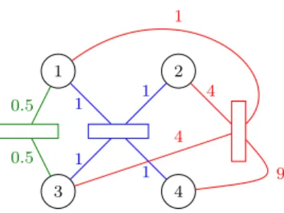
1 INTRODUCTION 2 3 1 2 4 1 1 1 1 0.5 0.5 4 1 9 4
Figure 1 – A hypernode graph modeling 3 tennis games with 4 players. Each of the three hyperedges has one color and models a game for which players connec-ted to the same long edge of a rectangle are in the same team.
where a hypernode is a set of nodes. Nodes in a hyper-node of a hyperedge are given a non negative weight that represents the node contribution to the binary re-lationship. An example of hypernode graph is presen-ted in Figure 1. There are four nodes that represent four tennis players and three hyperedges representing three games between teams : {1} against {3}, {1, 2} against {3, 4}, and {1, 4} against {2, 3}. For each hy-peredge, each player has been given a weight which can be seen as the player’s contribution. It can be no-ted that the hyperedge between singleton sets {1} and {3} can be viewed as an edge between nodes 1 and 3 with edge weight 1. Undirected graphs are shown to be hypernode graphs where hypernodes are singleton sets. Given a hypernode graph modeling binary relation-ships between sets of individuals, an important task, as said above, is to evaluate individuals by means of node labelling or node scoring functions. The se-cond contribution of this paper is to propose machine learning algorithms in the semi-supervised, batch set-ting on hypernode graphs for predicset-ting node labels or node scores. To this aim, we develop a spectral lear-ning theory for hypernode graphs. Similarly to the case of graph spectral learning, our approach relies on the assortative mixing (or homophilic) assumption which says that two linked nodes should have the same la-bel or similar scores. For graphs, this assumption is reflected in the choice of smooth node functions for which linked nodes get values that are close enough. For hypernode graphs, we assume an additive model, and we will say that a real-valued node function over a hypernode graph is smooth if, for linked hypernodes, the weighted sum of function values over the two node sets are close enough. As an example, let us consider the blue hyperedge in Figure 1 between the two sets
{1, 2} and {3, 4} and a real-valued node function f , the function f is said to be smooth over the hyperedge if f (1) + f (2) is close to f (3) + f (4).
For defining the smoothness, we introduce an unnor-malized gradient for hypernode graphs. Then, we define an unnormalized Laplacian ∆ for hypernode graphs by ∆ = GTG where G is the gradient. We show that the class of hypernode graph Laplacians is the class of symmetric positive semidefinite real-valued matrices M such that 1 ∈ Null(M ), where Null(M ) denotes the null space of M . This result allows to show that there exist hypernode graphs whose Laplacian matches that of a graph and that there exist hypernode graph Lapla-cians which are not the graph Laplacian of any graph. While it has been proved in [1] that hypergraph La-placians can be defined from graph LaLa-placians using adequate graph construction. Then, the smoothness of a real-valued node function f on a hypernode graph can be characterized by the smoothness semi-norm defined by Ω(f ) = fT∆f . We define the kernel of a hypernode graph to be the Moore-Penrose pseudoinverse of its La-placian. The spectral theory for hypernode graphs and its properties allow us to use spectral graph learning algorithms [14, 16, 18] for hypernode graphs.
We apply hypernode graph spectral learning to the rating of individual skills of players and to the pre-diction of game outcomes in multiple players games. We consider competitive games between two teams where each team is composed of an arbitrary number of players. Each game is modeled by a hyperedge and a set of games is represented by a hypernode graph. We define a skill rating function of players as a real-valued node function over the hypernode graph. And we show that finding the optimal skill rating function reduces to finding the real-valued function s∗ minimi-zing Ω(s) = sT∆s, where ∆ is the unnormalized
La-placian of the hypernode graph. The optimal indivi-dual skill rating function allows to compute the ra-ting of teams and to predict game outcomes for new games. We apply this learning method on real datasets of multiple player games to predict game outcomes in a semi-supervised, batch setting. Experimental results show that we obtain very competitive results compa-red to specialized algorithms such as Elo duelling and TrueSkill.
Related Work. Hypernode graphs that we introdu-ced can be viewed as an undirected version of directed hypergraphs popularized by [5] where a directed hy-peredge consists in an oriented relation between two sets of nodes. As far as we know, this class of direc-ted hypergraphs has not been studied from the
ma-2 GRAPHS AND HYPERNODE GRAPHS 3
chine learning point of view and no attempt was made to define a spectral framework for these objects. Hy-pernode graphs can also be viewed as an extension of (classical) hypergraphs. The question of learning with hypergraphs has been studied and, for an overview, we refer the reader to [1]. In this paper, the authors show that various formulations of the semi-supervised and the unsupervised learning problem on hypergraphs can be reduced to graph problems. For instance, the hyper-graph Laplacian of [17] can be defined as a hyper-graph La-placian by an adequate graph construction. To the best of our knowledge, no hypergraph Laplacian which can not be reduced to a graph Laplacian has been defined so far. A very recent tentative to fully use the hyper-graph structure was proposed by [7]. In this paper, the authors propose to use the hypergraph cut, and they introduce the total variation on a hypergraph as the Lovasz extension of the hypergraph cut. This allows to define a regularization functional on hypergraphs for defining semi-supervised learning algorithms.
2
Graphs
and
Hypernode
Graphs
2.1
Undirected Graphs and Laplacians
In the following, we recall the commonly accepted definitions of undirected graphs and graph Laplacians. An undirected graph g = (V, E) is a set of nodes V with |V | = n together with a set of undirected edges E with |E| = p. Each edge e ∈ E is an unordered pair {i, j} of nodes and has a non negative weight wi,j. In order to
define the smoothness of a real-valued node function f over a graph g, we define the gradient function grad for f by, for every edge (i, j),
grad(f )(i, j) =√wi,j(f (j) − f (i)) .
We can note that | grad(f )(i, j)| is small whenever f (i) is close to f (j). Then, the smoothness of a real-valued node function f over a graph g is defined by
Ω(f ) = X
i,j∈V2
| grad(f )(i, j)|2= fTGTGf ,
where G is the matrix of the linear mapping grad from Rn into Rp. The symmetric matrix ∆ = GTG is called undirected graph Laplacian, which is also proved to be defined by ∆ = D − W where D is the degree matrix of g and W the weight matrix of g. Ω(f ) = fT∆f has
been used in multiple works (see for example [18, 14]) to ensure the smoothness of a node labeling functionf .
Additional information concerning the discrete ana-lysis on graphs can be found in [16], which develop a similar theory with a normalized version of the gradient and Laplacian (G is replaced by GD−1/2).
2.2
Hypernode Graphs
The following definition is our contribution to the modeling of binary relationships between sets of enti-ties.
Definition 1 A hypernode graph h = (V, H) is a set of nodes V with |V | = n and a set of hyperedges H with |H| = p. Each hyperedge h ∈ H is an unordered pair {sh, th} of two non empty and disjoint hypernodes (a
hypernode is a subset of V ). Each hyperedge h ∈ H has a weight function wh mapping every node i in sh∪ th
to a positive weight wh(i) (for i /∈ sh∪ th, we define
wh(i) = 0). Each weight function wh of h = {sh, th}
must satisfy the Equilibrium Condition defined by X i∈th p wh(i) = X i∈sh p wh(i) .
An example of hypernode graph is shown in Figure 1. The red hyperedge links the sets {1, 4} and {2, 3}. The weights satisfy the Equilibrium condition which en-sures that constant node functions have a null gradient as we will see in the next section. The green hyperedge is an unordered pair {{1}, {3}} of two singleton sets with weights 0.5 for the nodes 1 and 3. It can be vie-wed as an edge between nodes 1 and 3 with edge weight 0.5. Indeed, when a hyperedge h is an unordered pair {{i}, {j}} involving only two nodes, the Equilibrium Condition states that the weights wh(i) and wh(j) are
equal. Thus, such a hyperedge can be seen as an edge with edge weight wi,j = wh(i) = wh(j). Therefore,
a hypernode graph such that every hyperedge is an unordered pair of singleton nodes can be viewed as an undirected graph, and conversely.
2.3
Hypernode graph Laplacians
We will define the smoothness of a real-valued node function f over a hypernode graph with the gradient that we define now.
Definition 2 Let h = (V, H) be a hypernode graph and f be a real-valued node function, the (hypernode graph) unnormalized gradient of h is a linear appli-cation, denoted by grad, that maps every real-valued node function f into a real-valued hyperedge function
2 GRAPHS AND HYPERNODE GRAPHS 4
grad(f ) defined, for every h = {sh, th} in H, by
grad(f )(h) =X i∈th f (i)pwh(i) − X i∈sh f (i)pwh(i) ,
where an arbitrary orientation of the hyperedges has been chosen.
As an immediate consequence of the gradient defi-nition and because of the Equilibrium Condition, the gradient of a constant node function is the zero-valued hyperedge function. Also, it can be noted that, for a hy-peredge h ∈ H, | grad(f )(h)|2is small when the weigh-ted sum of the values f (i) for nodes i in sh is close to
the weighted sum of the values f (j) for nodes j in th.
Thus, if we denote by G ∈ Rp×n the matrix of grad,
the smoothness of a real-valued node function f over a hypernode graph h is defined by Ω(f ) = fTGTGf .
Let h be a hypernode graph with unnormalized gra-dient G, the square n × n real valued matrix ∆ = GTG
is defined to be the unnormalized Laplacian of the hy-pernode graph h. It should be noted that the Laplacian ∆ does not depend on the arbitrary orientation of the hyperedges used for defining the gradient. When the hypernode graph is a graph, the unnormalized hyper-node graph Laplacian matches the unnormalized graph Laplacian. Last, we define the hypernode graph kernel of a hypernode graph h to be the Moore-Penrose pseu-doinverse ∆† of the hypernode graph Laplacian ∆.
2.4
Hypernode Graph Laplacians and
Learning
We can characterize hypernode graph Laplacians by Proposition 1 The class of hypernode graph Lapla-cians is the class of symmetric positive semidefinite real-valued matrices M such that 1 ∈ Null(M ), where Null(M ) denotes the null space of M .
Proof. It is an immediate consequence of the defini-tions of the hypernode graph gradient and the hyper-node graph Laplacian that a hyperhyper-node graph Lapla-cian is a symmetric positive semidefinite real-valued matrix, and that a constant function has a null gra-dient. For the other direction, let us consider a sym-metric positive semidefinite real-valued matrix M such that 1 ∈ Null(M ). Then, consider a square root de-composition M = GTG of M . For each line of G, one
can define a hyperedge h = {sh, th} with sh the set of
nodes with positive values in the line of G, ththe set of
nodes with negative values in the line of G, and weights equal to the square of values in the line of G. The Equi-librium condition is satisfied because 1 ∈ Null(M ) and
it is easy to verify that the Laplacian of the resulting hypernode graph h is M .
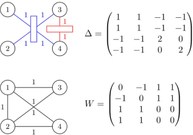
As a consequence of the construction in the previous proof, it should be noted that there are several hyper-node graphs with the same hyperhyper-node graph Laplacian because the square root decomposition is not unique. One can also find hypernode graphs whose Laplacian matches that of a graph. One can prove that this is not however the general case. For this, it suffices to consider a hypernode graph Laplacian with an extra-diagonal term which is positive. For instance, consider the hypernode graph and its Laplacian matrix ∆ in Figure 2, the Laplacian matrix has 1 as extradiagonal term, thus ∆ is not a graph Laplacian.
As said in Proposition 1, hypernode graph Lapla-cians are positive semidefinite. This allows to leve-rage most of the spectral learning algorithms defined in [14, 16, 18] from graphs to hypernode graphs. While it should be noted that hypernode graph Laplacians are stricly more general than graph Laplacians. Conse-quently, spectral hypernode graph learning can not be reduced to spectral graph learning.
2.5
Hypernode Graph Laplacians and
Signed Graphs
In this section we present additional properties of hypernode graph kernels. As in the graph case, we have defined the kernel of a hypernode graph to be the Moore-Penrose pseudoinverse of its Laplacian. Be-cause the pseudoinversion preserves semidefiniteness and symmetry, as a consequence of Proposition 1, one can show that the class of hypernode graph kernels is closed under the pseudoinverse operation. As a conse-quence, the class of hypernode graph kernels is equal to the class of hypernode graph Laplacians. It is worth noticing that the class of graph kernels is not closed by pseudoinversion.
It can also be shown that the class of hypernode graph Laplacians is closed by convex linear combina-tion. This is an important property in the setting of learning from different sources of data. As graph ker-nels are hypernode graph kerker-nels, it should be noted that the convex linear combination of graph kernels is a hypernode graph kernel, while it is not a graph ker-nel in general because the class of graph kerker-nels is not closed by convex linear combination. This explains why problems for hypernode graphs can not be solved using graph constructions.
We have shown above that there does not exist in general a graph whose Laplacian is equal to the Lapla-cian of a given hypernode graph. Nevertheless, given a
3 HYPERNODE GRAPH MODEL FOR MULTIPLE PLAYERS GAMES 5 1 2 3 4 1 1 1 1 1 1 1 2 3 4 -1 1 1 1 1 ∆ = 1 1 −1 −1 1 1 −1 −1 −1 −1 2 0 −1 −1 0 2 W = 0 −1 1 1 −1 0 1 1 1 1 0 0 1 1 0 0
Figure 2 – A hypernode graph, its Laplacian ∆ and its corresponding signed graph (right)
hypernode graph h, one can define a symmetric matrix W of possibly negative weights for pairs of nodes of h such that the hypernode graph Laplacian of h is equal to D−W , where D is the degree matrix associated with W . This means that there is a unique signed graph with weight matrix W such that D − W is the hypernode graph Laplacian of h. The construction is illustrated in Figure 2. This result highlights the subclass of si-gned graphs whose Laplacian computed with the for-mula D − W is positive semidefinite. This result also shows that homophilic relations between sets of nodes lead to non homophilic relations between nodes. It can also be shown that the hypernode graph cut defined as the binary restriction of the Laplacian regularization Ω(f ) = fT∆f is equivalent to the signed cut defined
on the corresponding signed graph. Namely, we have ∀C ⊆ V, Ω(1C) =Pi∈C,j /∈CWi,j, where 1C(i) = 1 if
and only if i ∈ C (0 otherwise).
3
Hypernode Graph Model for
Multiple Players Games
We consider competitive games between two teams where each team is composed of an arbitrary number of players. A first objective is to compute the skill ratings of individual players from game outcomes. A second objective is to predict a game outcome from a batch of games with their outcomes. For that, we will model games by hyperedges assuming that the performance of a team is the sum of the performances of its members as done by the team model proposed in [8].
3.1
Multiplayer Games
Let us consider a set of individual players P = {1, . . . , n} and a set of games Γ = {γ1, . . . , γp}
bet-ween two teams of players. Let us also consider that a player i contributes to a game γj with a non negative
weight wj(i). We assume that each player has a skill
s(i) and that a game outcome can be predicted by com-paring the weighted sum of the skills of the players of each of the two teams. More formally, given two teams of players A = {a1, a2, . . . , a`} and B = {b1, b2, . . . , bk}
playing game γj, then A is the winner if and only if ` X i=1 wj(ai)s(ai) > k X i=1 wj(bi)s(bi) . (1)
Equivalently, one can rewrite this inequality by in-troducing a non negative variable oj on the right hand
side such that :
` X i=1 wj(ai)s(ai) = oj+ k X i=1 wj(bi)s(bi) , (2)
where oj can be viewed as a variable quantifying the
game outcome. In the case of a draw oj = 0. Given
a set of games, it may be impossible to assert that all constraints (1) can be simultaneously satisfied. Our goal is to estimate a skill rating function s ∈ Rn that respects the game outcomes of the games in Γ as much as possible. We define the cost of a game γj with
out-come oj for a skill function s by
Cγj(s) = k ` X i=1 wj(ai)s(ai) − k X i=1 wj(bi)s(bi) − ojk2 .
Consequently, given a set of games Γ and the cor-responding game outcomes, the goal is to find a skill rating function s∗ that minimizes the sum of the dif-ferent costs, i.e. search for
s∗= arg min
s
X
γj∈Γ
Cγj(s) . (3)
3.2
Modeling Games with Hypernode
Graphs
In order to model multiplayer games with hypernode graphs, we represent players by nodes, teams by sets of nodes and each game by a hyperedge. Formally, let us consider a game γj between teams A and B in a set
of games Γ. We define the hyperedge hj for game γj as
3 HYPERNODE GRAPH MODEL FOR MULTIPLE PLAYERS GAMES 6 a1 . . . a` b1 . . . bk Zj Hj wj(a1)2 wj(a`)2 wj(b1)2 wj(bk)2 wj 1 2 1 3 4 Z H 1 1 1 1 1 1
Figure 3 – [top] Generic hyperedge hj for a game
γj between team A = {a1, . . . , al} and team B =
{b1, . . . , bk} and [bottom] hyperedge h for a game γ
between team A = {1, 2} and B = {3, 4} with node contributions set to 1
1. The players of team A correspond to one of the two hypernodes of hj. The weight of a player node
is the square of the contribution of the player in the game,
2. do the same construction for team B and the se-cond hypernode of hj
3. add a node Hj, called outcome node to the set of
player nodes corresponding to the losing team. The weight of this node is set to 1,
4. add a new node Zj, called 0-performance node to
the set of player nodes corresponding to the win-ning team. The weight wj of this node is chosen
in order to ensure the Equilibrium condition for the hyperedge hj.
A graphical representation of this construction is gi-ven in Figure 3.
Skill rating functions for players are real-valued node functions over the hypernode graph. In order to model the game outcomes in the computation of the skills, we fix some values in the corresponding node func-tion : each 0-performance node has value 0 ; the out-come node of game γj has the fixed value oj (recall
that oj is the outcome of game γj, see Eq (2)). As
an example, let us consider a game γ between two teams A = {1, 2} and B = {3, 4} and let us sup-pose that A wins the game. The corresponding hyper-edge h is presented in Figure 3 [bottom]. The skill ra-ting function must satisfy s(1) + s(2) > s(3) + s(4). We consider a node-valued function f on h such that f (Z) = 0 and f (H) > 0. The function f is smooth
on the hyperedge h if f (1) + f (2) + f (Z) is close to f (3) + f (4) + f (H). Then the smoothness of f allows to express that f (1) + f (2) > f (3) + f (4) and the dif-ference between the two team evaluations relies on the game outcome encoded in f (H). Thus, a smooth real-valued node function on the hyperedge h satisfies the constraints required for a skill rating function for the game γ.
Hypernode graph for a set of games and the skill rating problem. Let us consider a set of games Γ, we define the hypernode graph h = (V, H) as the set of all hyperedges hj for the games γj in Γ as defined
above. We assume a numbering of V such that V = {1, . . . , N } where N is the total number of nodes, the first n nodes are the player nodes followed by the t 0-performance nodes and the outcome nodes, that is, V = {1, . . . , n} ∪ {n + 1, . . . , n + t} ∪ {n + t + 1, . . . , N }. Let ∆ be the unnormalized Laplacian of h, and let s be a real-valued node function on h. s can be seen as a real vector in RN where the first n entries represent the skills of the n players. The skill rating problem (3) is equivalent to find the optimal vector s solving the optimization problem
minimize
s∈RN s
T∆s
subject to ∀n + 1 ≤ j ≤ n + t, s(j) = 0 (for 0-performance nodes) ∀n + t + 1 ≤ j ≤ N, s(j) = oj
(for outcome nodes)
(4)
3.3
Regularizing the hypernode graph
When the number of games is small, many players will participate to at most one game. Thus, in this case, the number of connected components can be quite large. The player skills in every connected com-ponent can be defined independently while satisfying the constraints. Thus, it will be unrelevant to compare player skills in different connected components. In or-der to solve this issue, we introduce in Equation (4) a regularization term based on the standard deviation of the players skills σ(sp) , where sp = (s(1), . . . , s(n)).
3 HYPERNODE GRAPH MODEL FOR MULTIPLE PLAYERS GAMES 7
This leads to the new formulation
minimize
s∈RN s
T∆s + µσ(s p)2
subject to ∀n + 1 ≤ j ≤ n + t, s(j) = 0 (for 0-performance nodes) ∀n + t + 1 ≤ j ≤ N, s(j) = oj
(for outcome nodes),
(5)
where µ is a regularization parameter. Thus, we control the spread of sp, avoiding to have extreme values for
players participating in a small number of games. In order to apply graph-based semi-supervised lear-ning algorithms using hypernode graph Laplacians, we now show that the regularized optimization problem can be rewritten as an optimization for some hyper-node graph Laplacian. For this, we will show that it suffices to add a regularization node in the hypernode graph h. First, let us recall that if s is the mean of the player skills vector sp = (s(0), . . . , s(n)), then for all
q ∈ R we have σ(sp)2= 1 n n X i=1 (s(i) − s)2≤ 1 n n X i=1 (s(i) − q)2 .
Thus, in the problem 5, we can instead minimize sT∆s +µ
n
Pn
i=1(s(i) − q)
2over s and q. We now show
that this can be written as the minimization of rT∆ µr
for some vector r and well chosen hypernode graph La-placian ∆µ. For this, let us consider the p × N gradient
matrix G of the hypernode graph h associated with the set of games Γ, and let us define the matrix Gµ by
Gµ = 0 0 G q µ nB ,
where B is the n × (N + 1) matrix defined by, for every 1 ≤ i ≤ n, Bi,i= −1, Bi,N +1= 1, and 0 otherwise. The
matrix Gµ is the gradient of the hypernode graph hµ
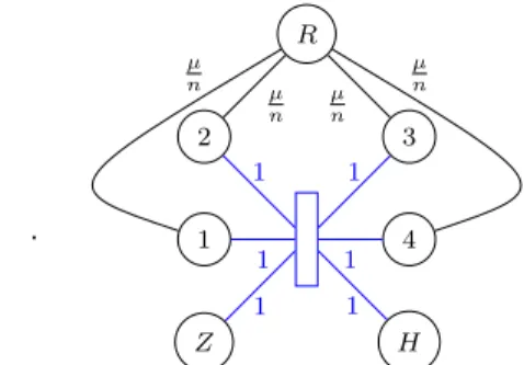
obtained from the hypernode graph h by adding a new node R, an hyperedge between every player node and R with node weights µ/n (such a hyperedge can be viewed as an edge with edge weight µ/n). The construction is illustrated in Figure 4 with a hypernode graph reduced to a single hyperedge.
Let us denote by r the vector (s(0), . . . , s(N ), q), then since ∆ = GTG, we can write
. 1 2 3 4 Z H 1 1 1 1 1 1 R µ n µ n µ n µ n
Figure 4 – Introducing a regularizer node R
rTGTµGµr = sT∆s + µ nrB TBr . As rBTBr = P i(si− q)2, if we denote by ∆µ = GT
µGµ the (N + 1) × (N + 1) unnormalized Laplacian
of the hypernode graph hµ, we can finally rewrite the
regularized problem (5) as minimize r∈RN +1 r T∆ µr subject to ∀n + 1 ≤ j ≤ n + t, r(j) = 0 (for 0-performance nodes) ∀n + t + 1 ≤ j ≤ N, r(j) = oj
(for outcome nodes)
(6)
3.4
Infering Skill Ratings and
Predic-ting Game Outcomes
We have shown that predicting skill ratings can be written as the optimization problem (6). It should be noted that it can also be viewed as a semi-supervised learning problem on the hypernode graph hµ because
the question is to predict node scores (skill ratings) for player nodes when node scores for 0-performance nodes and outcome nodes are given. Using Proposition 1), we get that ∆µ is a positive semidefinite real-valued
ma-trix because it is a hypernode graph Laplacian. The-refore, we can use the semi-supervised learning algo-rithm presented in [18]. This algoalgo-rithm was originally designed for graphs and solves exactly the problem (6) by putting hard constraints on the outcome nodes and on the 0-performance nodes. We denote this method by H-ZGL.
In order to predict skill ratings, another approach is to infer player node scores from 0-performance nodes scores and outcome nodes scores nodes using a regres-sion algorithm. For this, we consider the hypernode graph kernel ∆†µ (defined as the Moore-Penrose pseu-doinverse of the Laplacian ∆µ) and train a regression
4 EXPERIMENTS 8
support vector machine. We denote this method by H-SVR.
Using the two previous methods, we can infer skill ratings for players from a given set of games. The infer-red skill ratings can be used to pinfer-redict game outcomes for new games. For this, we suppose that we are given a training set of games Γl with known outcomes
to-gether with a set of testing games Γu for which game
outcomes are not known. The goal is to predict game outcomes for the testing set Γu. Note that other works
have considered similar questions in the online setting as in [8, 4] while we consider the batch setting. For the prediction of game outcomes, first we apply a skill rating prediction algorithm presented above given the training set Γl and output a skill rating function s∗.
Then, for each game in Γu, we evaluate the
inequa-lity (1) with the skills defined by s∗ and decide the winner. For every player which do not appear in the training set, the skill value is fixed a priori to the mean of known player skills.
Algorithm 1 Predicting game outcomes
Input: Training set of games Γl, set of testing games
Γu
1: Build the regularized hypernode graph hµ based
on Γl as described in Sections 3.2 and 3.3
2: Compute an optimal skill rating s∗ using H-ZGL or H-SVR.
3: Compute the mean skill ˜s among players in Γl
4: for each game in Γu do
5: Assign skill given by s∗ for players involved in Γl, and ˜s otherwise
6: Evaluate the inequality (1) and predict the win-ner
7: end for
4
Experiments
In this section, we report experimental results for the inference of individual skills and the prediction of game outcomes for different datasets.
4.1
Tennis Doubles
We consider a dataset of tennis doubles collected between January 2009 and September 2011 from ATP tournaments (World Tour, Challengers and Futures). Tennis doubles are played by two teams of two players. Each game has a winner (no draw is allowed). A game is played in two or three winning sets. The final score
corresponds to the number of sets won by each team during the game. The dataset consists in 10028 games with 1834 players.
In every experiment, we select randomly a training subset Γl of games and all remaining games define a
testing subset Γu. We will consider different sizes for
the training set Γl and will compute the outcome
pre-diction error on the corresponding set Γu. More
pre-cisely, for a given proportion ρ varying from 10% to 90% , we build a training set Γlusing ρ% of the games
chosen randomly among the full game set, the remai-ning games form the test set Γu. We present in Figure
5 and 6 several statistics related to the Tennis dataset. It is worth noticing that many players have played only once. Therefore, the skill rating problem and the game outcome prediction problem become far more difficult to solve when few games are used for learning. Moreo-ver, it should be noted that when the number of games in the training set is small, the number of players in the test set which are involved in a game of the trai-ning set is small. In this case many players will have a skill estimated to be the average skill. This explains why the problem is difficult when the number of games in Γl is small.
Given a training set of games Γland a test set Γu, we
follow the experimental process described in Algorithm 1. For the definition of the hypergraph, we fix all player contributions in games to 1 because we do not have ad-ditional information than final scores. Thus the player nodes weights in every hyperedge is 1. In the optimi-zation problem 6, the game outcomes oj are defined to
be the difference between the number of sets won by the two teams. This allows to take account of the score when computing player skills. In order to reduce the number of nodes in our hypernode graph, we merge all the 0-performance nodes in a single one that is shared by all the hyperedges. We do the same for outcome nodes because score differences can be 1, 2 or 3. The resulting hypernode graph has at most 1839 nodes : at most 1834 player nodes, 1 shared 0-performance node, 3 outcome nodes, and 1 regularizer node.
To complete the definition of the hypernode graph hµ constructed from the game set Γl, it remains to
fix the parameter value for µ/n. For this, assuming a Gaussian distribution for skill ratings and comparing expected values for the two terms sT∆s and µσ(s
p)2,
we show (see Appendix A) that the value of µ/n should have the same order of magnitude than the average number of games played by a player. We fix the default value to be 16 for µ/n and use this default value in all experiments.
4 EXPERIMENTS 9 0 100 200 300 400 500 600 700 0 10 20 30 40 50 60 Num b er of pla y ers Played games
Figure 5 – Distribution of the number of players against the number of played games
40 50 60 70 80 90 100 0.1 0.2 0.3 0.4 0.5 0.6 0.7 0.8 0.9 P erce n tage of kno wn pla y ers in Γu
Proportion of games used for Γl
Figure 6 – Average percentage of players in Γu which
are involved in some game in Γl
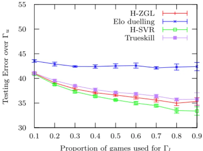
rating prediction algorithms H-ZGL and H-SVR. In or-der to compare our method, we also infer skill ratings using Elo Duelling and Trueskill [8]1Then, we predict
game outcomes from the inferred skill ratings. The re-sults are given in Figure 7 (for each value of ρ, we repeat the experiment 10 times). It can be noted that Elo duelling performs poorly. Also, it can be noted that H-ZGL is significantly better than Trueskill whatever is the chosen proportion.
4.2
Xbox Title Halo2
The Halo2 dataset was generated by Bungie Studio during the beta testing of the XBox title Halo2. It has been notably used in [8] to evaluate the performance of the Trueskill algorithm. We consider the Small Teams 1. TrueSkill and Elo implementations are from [6]. Results were double-checked using [13] and [12]. Parameters of Elo and TrueSkill are the default parameters of [6] (K = 32 for Elo, µ0= 25, β = 12.5, σ = 8.33 and τ = 0.25 for TrueSkill).
30 35 40 45 50 0.1 0.2 0.3 0.4 0.5 0.6 0.7 0.8 0.9 T esting Err or o v e r Γu
Proportion of games used for Γl
H-ZGL Elo duelling H-SVR Trueskill
Figure 7 – Predictive error depending on the propor-tion of games used to build Γl
dataset with 4992 players and 27536 games opposing up to 12 players in two teams. It should be noted that a game can confront two teams of different size. Each game can result in a draw or a win of one of the two teams. The proportion of draws is 22.8%. As repor-ted in [8], the prediction of draws is challenging and it should be noted that Trueskill and our algorithm fail to outperform a random guess for the prediction of draw. We again consider the experimental process descri-bed in Algorithm 1. As for the Tennis dataset, we fix all players contributions in games to 1. In the optimi-zation problem 6, the game outcomes oj are defined to
be equal to 1 when the game has a winner and 0 other-wise. This is because game scores in the dataset vary depending on the type of game considered. As above, we merge the 0-performance nodes into a single one and do the same for outcome nodes. The value of µ/n is again set to 16.
We use the experimental process defined for the Ten-nis dataset in order to compare the skill rating al-gorithms H-ZGL, H-SVR, Elo Duelling and Trueskill. The number of prediction errors for game outcomes is computed assuming that a draw can be regarded as half a win, half a loss [11]. We present the experimental results in Figure 8. For a proportion of 10% of games in the training set, H-ZGL, H-SVR and Trueskill give similar results. While with larger training sets, our hy-pernode graph learning algorithms outperform Trues-kill. On the Small Teams dataset, the inference of the skill rating function with hypernode graphs is achieved in less than 2 minutes.
R ´EF ´ERENCES 10 30 35 40 45 50 55 0.1 0.2 0.3 0.4 0.5 0.6 0.7 0.8 0.9 T esti ng Error o v er Γu
Proportion of games used for Γl
H-ZGL Elo duelling H-SVR Trueskill
Figure 8 – Predictive error depending on the propor-tion of games used to build Γl
5
Conclusion
We have introduced a new class of undirected hyper-graphs modeling pairwise relationships between sets of individuals. The class of hypernode graphs strictly ex-tends the class of graphs while keeping important pro-perties for the design of machine learning algorithms. For instance, Laplacians and kernels have been gene-ralized to hypernode graphs allowing to define semi-supervised learning algorithms for hypernode graphs in the spirit of [16]. We have applied our work to the problem of skill rating and game outcome prediction in multiple players games and obtained very promising results.
From a theoretical perspective, it should be inter-esting to study more deeply the notion of cut for our class of hypernode graphs. Recent work by [7] could be a promising line of research in order to design an ade-quate definition of cuts. From a machine learning pers-pective, we should define online learning algorithms for hypernode graphs following [9]. Also, we should consi-der normalized Laplacians. Last, we are confident in the capability of our model to handle new applications in networked data.
R´
ef´
erences
[1] Sameer Agarwal, Kristin Branson, and Serge Be-longie. Higher order learning with graphs. In Proc. of ICML, pages 17–24, 2006.
[2] Claude Berge. Graphs and hypergraphs. North-Holl Math. Libr. North-North-Holland, Amsterdam,
1973.
[3] Jie Cai and Michael Strube. End-to-end corefe-rence resolution via hypergraph partitioning. In Proc. of COLING, pages 143–151, 2010.
[4] Arpad Emrick Elo. The Rating of Chess Players, Past and Present. Arco Publishing, 1978.
[5] Giorgio Gallo, Giustino Longo, Stefano Pallottino, and Sang Nguyen. Directed hypergraphs and ap-plications. Discrete Applied Mathematics, 42(2-3) :177–201, 1993.
[6] Scott Hamilton. PythonSkills : Implementation of the trueskill, glicko and elo ranking algorithms. https://pypi.python.org/pypi/skills, 2012. [7] Matthias Hein, Simon Setzer, Leonardo Jost, and
Syama Sundar Rangapuram. The total variation on hypergraphs - learning on hypergraphs revisi-ted. In Proc. of NIPS, pages 2427–2435, 2013. [8] Ralf Herbrich, Tom Minka, and Thore Graepel.
Trueskilltm : A bayesian skill rating system. In Proc. of NIPS, pages 569–576, 2006.
[9] Mark Herbster and Massimiliano Pontil. Predic-tion on a graph with a perceptron. In Proc. of NIPS, pages 577–584, 2006.
[10] Steffen Klamt, Utz-Uwe Haus, and Fabian Theis. Hypergraphs and cellular networks. PLoS Com-putational Biology, 5(5), May 2009.
[11] Jan Lasek, Zolt´an Szl´avik, and Sandjai Bhulai. The predictive power of ranking systems in asso-ciation football. International Journal of Applied Pattern Recognition, 1(1) :27–46, 2013.
[12] Heungsub Lee. Python implementation of Elo : A rating system for chess tournaments. https: //pypi.python.org/pypi/elo/0.1.dev, 2013. [13] Heungsub Lee. Python implementation of
TrueS-kill : The video game rating system. http:// trueskill.org/, 2013.
[14] Ulrike Von Luxburg. A tutorial on spectral clus-tering. Statistics and computing, 17(4) :395–416, 2007.
[15] Shujun Zhang, Geoffrey D. Sullivan, and Keith D. Baker. The automatic construction of a view-independent relational model for 3-d object re-cognition. Pattern Analysis and Machine Intel-ligence, IEEE Transactions on, 15(6) :531–544, 1993.
[16] Dengyong Zhou, Jiayuan Huang, and Bernhard Sch¨olkopf. Learning from labeled and unlabeled data on a directed graph. In Proc. of ICML, pages 1036–1043, 2005.
R ´EF ´ERENCES 11
[17] Dengyong Zhou, Jiayuan Huang, and Bernhard Sch¨olkopf. Learning with hypergraphs : Cluste-ring, classification, and embedding. In Proc. of NIPS, pages 1601–1608, 2007.
[18] Xiaojin Zhu, Zoubin Ghahramani, John Lafferty, et al. Semi-supervised learning using gaussian fields and harmonic functions. In Proc. of ICML, volume 3, pages 912–919, 2003.
![Figure 3 – [top] Generic hyperedge h j for a game γ j between team A = {a 1 , . . . , a l } and team B = {b 1 ,](https://thumb-eu.123doks.com/thumbv2/123doknet/14526866.532612/7.918.175.377.99.343/figure-generic-hyperedge-game-γ-team-team-b.webp)