The electric vehicle routing problem with capacitated charging stations

HAL Id: hal-02386167

https://hal.archives-ouvertes.fr/hal-02386167v2

Preprint submitted on 15 Feb 2021

HAL is a multi-disciplinary open access

archive for the deposit and dissemination of

sci-entific research documents, whether they are

pub-lished or not. The documents may come from

teaching and research institutions in France or

abroad, or from public or private research centers.

L’archive ouverte pluridisciplinaire HAL, est

destinée au dépôt et à la diffusion de documents

scientifiques de niveau recherche, publiés ou non,

émanant des établissements d’enseignement et de

recherche français ou étrangers, des laboratoires

publics ou privés.

The electric vehicle routing problem with capacitated

charging stations

Aurélien Froger, Ola Jabali, Jorge E. Mendoza, Gilbert Laporte

To cite this version:

Aurélien Froger, Ola Jabali, Jorge E. Mendoza, Gilbert Laporte. The electric vehicle routing problem

with capacitated charging stations. 2021. �hal-02386167v2�

The electric vehicle routing problem with capacitated charging

stations

Aur´

elien Froger

_{Ola Jabali}

_{Jorge E. Mendoza}

_{Gilbert Laporte}

1_{Universit´e de Bordeaux, UMR CNRS 5251 – Inria Bordeaux Sud-Ouest}

2_{Dipartimento di Elettronica, Informazione e Bioingegneria, Politecnico di Milano, Milan, Italy} 3_{HEC Montr´eal, Montr´eal, Canada}

4_{School of Management, University of Bath, Bath, United Kingdom}

Submitted for publication in December 2020 Abstract

Electric vehicle routing problems (E-VRPs) deal with routing a fleet of electric vehicles (EVs) to serve a set of customers, while minimizing an operational criterion, e.g., cost or time. The feasibility of the routes is constrained by the autonomy of the EVs, which may be recharged along the route. Much of the E-VRP research neglects the capacity of charging stations (CSs), and thus implicitly assumes that an unlimited number of EVs can be simultaneously charged at a CS. In this paper, we model and solve E-VRPs considering these capacity restrictions. In particular, we study an E-VRP with non-linear charging functions, multiple charging technologies, en route charging, and variable charging quantities, while explicitly accounting for the number of chargers available at privately managed CSs. We refer to this problem as the E-VRP with non-linear charging functions and capacitated stations (E-VRP-NL-C). We introduce a continuous-time model formulation for the problem. We then introduce an algorithmic framework that iterates between two main components: 1) The route generator, which uses an iterated local search algorithm to build a pool of high-quality routes and 2) The solution assembler, which applies a branch-and-cut algorithm to combine a subset of routes from the pool into a solution satisfying the capacity constraints. We compare four assembly strategies on a set of instances. We show that our algorithm effectively deals with the E-VRP-NL-C. Furthermore, considering the uncapacitated version of the E-VRP-NL-C, our solution method identifies new best-known solutions for 80 out of 120 instances.

Keywords— Electric vehicle routing; non-linear charging function; synchronization constraints; mixed integer linear programming; matheuristic; iterated local search; branch-and-cut

1

Introduction

In recent years, competitive prices and technological advances have made electric vehicles (EVs) an attractive alternative to internal combustion engine-powered vehicles for logistics operations (Juan et al., 2016; Pelletier et al., 2016). To allow companies and private vehicle users to fully integrate EVs in their operations and their trips, the operations research community has turned its attention to EV route planing. The resulting literature can be divided into two streams: optimal path and vehicle routing problems. As the name suggests, the first stream focuses on problems in which the objective is to find an optimal path from an origin to a destination on a road network, while taking into account the EV’s short driving range and accommodating stops at charging stations (CSs) to recharge the vehicle’s battery. These problems are out of the scope of this paper, but we refer the reader to the works of Baum et al. (2019) and Baum et al. (2020) for a thorough literature review and a state-of-the-art results for these problems. We focus on the second stream, namely, electric vehicle routing problems (E-VRPs).

E-VRPs consist of designing routes to serve a set of customers using a fleet of EVs. Due to their relatively short driving range, EVs may need to detour to CSs to replenish their battery. This is especially critical in the context of

mid-haul or long-haul routing (Schiffer et al., 2018b; Villegas et al., 2018). Therefore, key decisions in E-VRPs concern not only the assignment of the customers to the vehicles and their sequencing, but also where and how much to charge the vehicles.

One of the main modeling elements in E-VRPs is the charging process of batteries. Some studies assume that EVs are fully recharged whenever they detour to a CS. That is the case, for instance, in the green vehicle routing problem (G-VRP). The G-VRP was introduced by Erdo˘gan and Miller-Hooks (2012) and tackled by Ko¸c and Karaoglan (2016), Montoya et al. (2016), Andelmin and Bartolini (2017), and Bruglieri et al. (2019a), among others. One of the main assumptions in the G-VRP is that the charging time is constant, meaning that the vehicle takes a fixed amount of time to charge the battery to its full capacity, independently of the initial state of charge (SoC). Authors such as Schneider et al. (2014) and Hiermann et al. (2016) relaxed this assumption and incorporated charging times that linearly depend on the SoC upon arrival at the CS. As Montoya et al. (2017) pointed out, the full charge policy may lead to unnecessary out-of-the-depot charging, which translates into expensive driver idling time and overpriced energy purchases. To overcome this drawback, several researchers have studied problem variants in which the charging time is a decision variable; notable examples include the work of Felipe et al. (2014) Desaulniers et al. (2016), Montoya et al. (2017), Keskin and C¸ atay (2018), and Froger et al. (2019). In the first two examples, the authors assume that the charge retrieved at a CS is a linear function of the charging time. In reality, however, the battery charging process follows a non-linear function with respect to time (Pelletier et al. (2017)). To account for this, Montoya et al. (2017), Ko¸c et al. (2018), and Froger et al. (2019) modeled the charging process using concave piecewise linear functions, while Lee (2020) considered a general concave and non-decreasing charging function. In the resulting problem, known as the electric vehicle routing problem with non-linear charging function (E-VRP-NL), the charging times no longer rely solely on the quantity of energy charged but also on the initial SoC of the EV.

In all the previously discussed research, the authors assume that CSs are always available to charge a vehicle, thus, implicitly assuming that CSs are uncapacitated and can simultaneously charge an unlimited number of EVs. In practice, however, each CS has a fixed and often small number of chargers. The intuition behind neglecting the CS capacity constraints is that accounting for the detour and charging times (or costs) while planning the routes is enough to capture the impact of the charging decisions on the cost and feasibility of solutions. Nonetheless, the long charging times (which may range from tens of minutes to several hours) and the small number of chargers typically available at CSs may generate congestion.

The nature of the congestion problem at CSs largely depends on the access options available to the fleet operator. For instance, a few networks of public (as in accessible to anyone) CSs allow for charging time reservations. In this case, congestion may be neglected and the fleet operator only needs to make sure that routes reach the CSs within the reserved time windows. To accurately model the availability of each charger at a CS, the fleet operator may also manage their allocation to the EVs within the reserved time windows (see for instance Bruglieri et al. (2019b) for an example). In practice, most public charging stations do not allow for reservations. In this case, the exact time at which EVs can access CSs is uncertain. Indeed, upon arrival, the chargers may be busy and the vehicle may have to wait in a queue or detour to a close by station. Keskin et al. (2019) dealt with this issue by explicitly considering expected (i.e., deterministic) time-dependent queuing times at CSs. Kullman et al. (2020) went a step further and proposed dynamic optimization policies that constantly adapt charging and routing decisions depending on the state of CS queues. While these authors demonstrated that their approaches can effectively handle CS access uncertainty, as Villegas et al. (2018) pointed out, most companies are unwilling to bear this risk, and thus decide to install their own private out-of-depot charging infrastructure (e.g., at satellite depots, company office branches, or exclusive-access parking spots in city centers).

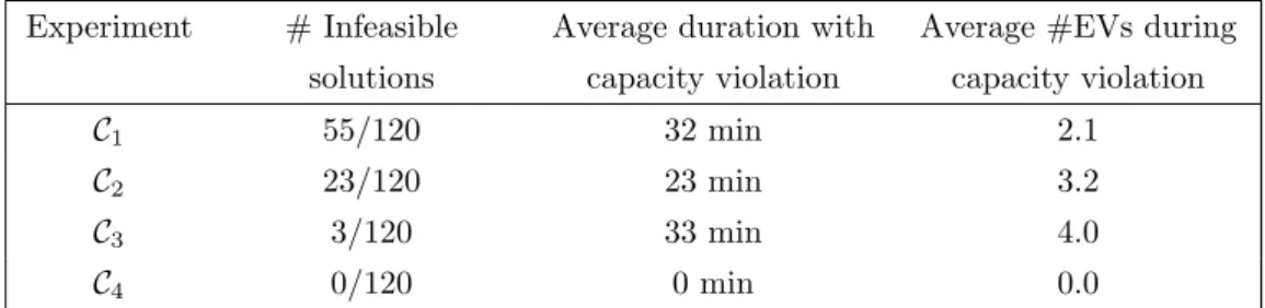
Relying on a privately operated charging infrastructure only changes the nature of the congestion problem, but does not solve it. To illustrate this point, we ran a feasibility test on the 120 best-known solutions (BKSs) for the E-VRP-NL reported in Montoya et al. (2017) limiting the number of chargers per CS to one, two, three, and four. According to our results, 55 of the BKSs become infeasible if there is only one charger per CS. This figure drops to 23 and three for the cases with two and three chargers. The only scenario where all BKSs are feasible is when CSs have four chargers (see Appendix A for details). Intuitively, one may think that by merely shifting the starting time of the charging operations, the feasibility problem will be solved. However, our experiments show that this is not only unnecessarily expensive (albeit with a very limited time increase), but more importantly it may be infeasible. Another option to

mitigate the effects of congestion is to increase the number of chargers installed at each CS, but this may not be a viable solution in practice. Indeed, Gnann et al. (2018) predict that by the end of 2020, the purchase and installation costs of a fast charging point (i.e., power rates above 22 kW) will be around 40,000e and its annual operation cost will reach 4,000e. Thus, if a company decides to invest in out-of-the-depot charging infrastructure, there is little chance that it will decide to install more than a couple of chargers at each CS. In conclusion, we argue that in most practical situations, the congestion at the CSs should be taken into account when planning the routes by explicitly modeling the capacity constraints.

We are aware of only one work taking into account CS capacity constraints when optimizing routing decisions in the context of a private charging infrastructure. Bruglieri et al. (2019b) extended the G-VRP to account for the number of pumps in the alternative refueling stations. They introduced a path-based formulation and solved it using a cutting plane algorithm. They reported optimal solutions on instances up to 20 customers. Out of the field of vehicle routing, some researchers have studied related problems. For instance, Sassi and Oulamara (2014) and Pelletier et al. (2018) considered the problem of scheduling charging operations at the depot, assuming that the routes are given as an input. Both papers considered not only constraints on the number of available chargers, but also electricity grid constraints limiting the amount of power that can be drawn from the electric grid at any given time. The latter is typically a binding constraint for central depots with a large number of available chargers, but is usually not a concern for CSs since they are designed to operate at full capacity. Brandst¨atter et al. (2020) studied the problem of finding optimal locations and sizes for charging stations based on the number of expected trips. They explicitly took charging station capacity into account using a time-expanded location graph.

In order to help the readers find their way through the different assumptions, Table 1 summarizes the main E-VRPs variants addressed in the literature (it excludes the literature on location-routing problems). The table is not exhaustive, but it provides a good overview of the current state of the research on E-VRPs.

In this paper we introduce the VRP-NL with capacitated CSs (VRP-NL-C). The problem extends classical E-VRPs to account for the fixed number of chargers available at each CS. We assume that the CSs are privately operated. Our research extends the work of Bruglieri et al. (2019b) by considering a more general charging function and charging policy, which introduces additional decisions. Specifically, rather than assuming that every EV is fully charged in constant time when it stops at a CS, the quantity of energy charged during every stop at a CS is a decision variable. Moreover, since charging functions are piecewise linear, the charging time of an EV depends on its initial SoC and the quantity of energy charged. Last but not least, we also propose an algorithm to tackle medium and large-size instances. The E-VRP-NL-C is a complex combined routing-scheduling problem belonging to the family of VRPs with syn-chronization constraints. More specifically, according to the taxonomy introduced by Drexl (2012), the E-VRP-NL-C belongs to the class of VRPs with resource synchronization, where vehicles compete to access scarce resources (i.e., the chargers at every CS). The E-VRP-NL-C shares similarities with problems where vehicles need to wait while the loading equipment is busy. Examples of problems in this class include the log truck scheduling problem (El Hachemi et al., 2013; Rix et al., 2015) and routing and scheduling problems arising in public works (Grimault et al., 2017). The E-VRP-NL-C also relates to VRPs with inter-tour resource constraints. In these problems, the scarce resources are located only at the terminal vertex of the routes (i.e., the depot). An example of a problem in this category is the VRP introduced by Hempsch and Irnich (2008), where there is a limited number of ramps at the depot, and therefore only a fixed number of vehicles can be served simultaneously. The problem that is most closely related to the E-VRP-NL-C is the VRP with location congestion introduced by Lam and Van Hentenryck (2016). In this problem, each customer has a given number of requests and a limited number of resources (e.g., conveyors). When a vehicle arrives at a customer location, it must wait until at least one resource becomes available to handle the shipping. However, there exist two fundamental differences between their problem and our E-VRP-NL-C. The first is that in our problem, visiting locations with limited resources (the CSs) is needed for feasibility reasons. As a consequence, not only the number, but also the location and duration of the charging operations depend on the configuration of the routes. In other words, the tasks that must be synchronized are not known a priori. The second difference is that in contrast to their problem, in our E-VRP-NL-C, the task synchronization has a direct impact on the solution cost.

The contribution of this paper is twofold. First, we propose a mixed integer linear programming (MILP) formulation for the E-VRP-NL-C, showing how CS capacity constraints can be integrated into a standard E-VRP model. Second, we introduce a framework to solve E-VRPs with CS capacity constraints in general, and the E-VRP-NL-C in particular.

Table 1: Summary of the literature on E-VRPs

Reference

Charging infrastructure Charging process

Fleet Model(s) Main algorithm Cong. | Access. Multiple Partial Function

speed policy

Erdo˘gan and Miller-Hooks (2012) NEG C H CS-Repl Heuristics Felipe et al. (2014) NEG X X L H CS-Repl Local-search heuristics Schneider et al. (2014) NEG L H CS-Repl Hybrid VNS/TS Goeke and Schneider (2015) NEG L M CS-Repl ALNS Schneider et al. (2015) NEG C/L H CS-Repl AVNS Desaulniers et al. (2016) NEG X L H SP Branch-and-price1 Hiermann et al. (2016) NEG L M CS-Repl, SP Branch-and-price + ALNS Keskin and C¸ atay (2016) NEG X L H CS-Repl ALNS Ko¸c and Karaoglan (2016) NEG C H CS-Repl, CS-Path-1 Simulated annealing + B&C Montoya et al. (2016) NEG C H - Multi-space sampling heuristic Montoya et al. (2017) NEG X X PL H CS-Repl Matheuristic Andelmin and Bartolini (2017) NEG C H SP (CS-Path) Two-phase exact algorithm Leggieri and Haouari (2017) NEG C H CS-Repl, CS-Path-1 B&C Keskin and C¸ atay (2018) NEG X X L H CS-Repl ALNS

Andelmin and Bartolini (2019) NEG C H CS-Path Multi-start local search heuristic Bruglieri et al. (2019a) NEG C H Customer-Path B&C (exact and heuristic) Bruglieri et al. (2019b) SCH | PUB-R/PO C H CS-Repl, Customer-Path B&C Froger et al. (2019) NEG X X PL H CS-Repl, CS-Path MILP Models Hiermann et al. (2019) NEG X L M - Matheuristic (genetic + SP) Macrina et al. (2019) NEG X X L M CS-Repl Iterated local search Lee (2020) NEG X Cv SV Customer-Path Branch-and-price Keskin et al. (2019) DWT | PUB X PL H CS-Repl ALNS + MILP for route enhancement Kullman et al. (2020) DYN | PUB/PO X X PL SV CS-Repl Static and dynamic policies Our research SCH | PO X X PL H CS-Path Matheuristic (ILS + B&C) 1 Improved results can be found in Desaulniers et al. (2020)

• Charging infrastructure:

– Strategy to deal with congestion at CSs and accessibility of CSs (Cong. | Access.): neglected (NEG), scheduling of charging operations according to the number of available chargers (SCH), deterministic time-dependent waiting times (DWT), dynamic decision making (DYN) | public (PUB) –accessible to anyone, public with reservation (PUB-R), privately operated (PO)

– Multiple speed: each station may charge at a different speed (e.g., fast, moderate, slow)

• Charging process:

– Partial policy: the quantity of energy charged is a decision

– Function: constant charging time (C), charging times linearly depending on the quantity of energy charged (L), charging times depending on the quantity of energy charged and on the initial SoC: concave piecewise linear charging function (PL), concave and non-decreasing charging function (Cv)

• Fleet: homogeneous (H), mixed (M), single vehicle (SV)

• Model(s): CS replication-based formulation (CS-Repl), path-based formulation in which each path corresponds to a sequence of stops at CSs between customers and/or the depot (CS-Path), CS-Path in which every path contains at most one stop at a CS (CS-Path-1), path-based formulation in which each path corresponds to a sequence of visits to customers between CSs and/or the depot (Customer-Path), classical set partitioning with a variable per route (SP)

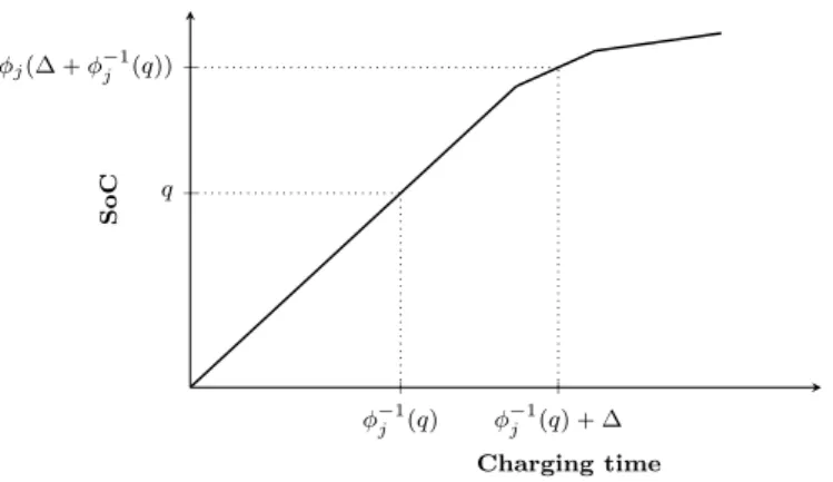
φ´1 j pqq φ ´1 j pqq ` ∆ q φjp∆ ` φ´1j pqqq Charging time SoC

Figure 1: Piecewise linear charging function of a CS j P F .

It is made up of two interacting components: a route generator and a solution assembler. The first component builds a set of high-quality solutions, while relaxing the capacity constraints. The routes making up these solutions are stored in a pool which is sent to the assembler every few iterations. The latter combines routes from the pool in an attempt to build a solution meeting the capacity constraints. If such a solution does not exist or cannot be found within a given computing time, the assembler sends a signal to the generator to modify the search space in order to favor feasibility. For the particular case of the E-VRP-NL-C, we have developed a route generator based on a new and efficient iterated local search (ILS) for the E-VRP-NL, and a solution assembler based on branch-and-cut. We present four assembly strategies allowing for different tradeoffs between efficiency and effectiveness. We have carried out extensive computational experiments on a large set of instances with different characteristics adapted from available benchmarks. The results demonstrate that our approach can handle the CS capacity constraints effectively. In addition, we report new BKS for 80 out of the 120 instances of a well-established benchmark set for the closely related E-VRP-NL. The remainder of this paper is organized as follows. Section 2 formally introduces the E-VRP-NL-C. Section 3 describes a MILP formulation of the problem. Section 4 presents the proposed solution method. Section 5 shows the computational results. Finally, Section 6 concludes and outlines research perspectives.

2

Problem description

We define the E-VRP-NL-C as follows. Let I be the set of customers that need to be served and let F be the set of CSs at which recharging can take place. The CSs are privately operated, meaning that there is no uncertainty on their availability. Each customer i P I has a service time gi. The customers are served using a homogeneous fleet of EVs.

Each EV has a battery of capacity Q (expressed in Wh). At the beginning of the planning horizon, the EVs are located in a single depot, from which they leave fully charged. The depot is continuously open for Tmax hours. Traveling from

one location i (the depot, a customer, or a CS) to another location j incurs a driving time tijě 0 that corresponds to

the shortest path in time from i to j and an energy consumption eijě 0 associated to this path.

Due to their limited battery capacity, EVs may need to stop en route at CSs. Charging operations can occur at any CS, they are non-preemptive, and EVs can be partially recharged. The CS j P F has a concave piecewise linear charging function φj that maps for an empty battery the time spent charging at j and the SoC of the vehicle upon

departing from j. If q is the SoC of the EV upon arrival at j and ∆ is the charging time, then the SoC of the EV upon departure from j is given by φjp∆ ` φ´1_j pqqq (Figure 1). We denote by Bj “ tpaj0, qj0q, . . . , pajbj, qjbjqu the totally

ordered set of breakpoints of the charging function at CS j, where every breakpoint is a (charging time, SoC) pair, sorted in non-decreasing order of time.

Each CS j P F also has a capacity, given by the number of available chargers Cj. Due to the limited capacity of

CSs, vehicles may incur waiting times while they queue for a charger. We therefore note that optimal solutions are not necessarily left-shifted schedules, as is the case for the E-VRP-NL and other E-VRP variants assuming uncapacitated CSs.

once by a single vehicle, 2) each route starts at the depot not before time 0 and ends at the depot not later than time Tmax, 3) each route is energy-feasible, i.e., the SoC of an EV when it enters and leaves from any location lies between

0 and Q, and 4) no more than Cj EVs simultaneously charge at each CS j P F . The objective of the E-VRP-NL-C is

to minimize the total time needed to serve all customers, including driving, service, charging, and waiting times. Note that to avoid congestion at CSs, the starting times of the routes can be delayed at no cost. Moreover, an E-VRP-NL-C instance may have no feasible solution.

3

A mixed-integer linear programming formulation

We can classify explicit the mixed integer linear programming formulations for E-VRPs into two categories: CS replication-based formulations and path-based formulations. CS replication-based formulations are the compact MILP formulations typically used in the E-VRP literature to mathematically define the problem and solve toy instances. As their name suggests, in these formulations the nodes representing CSs are replicated and the number of stops at each CS replication is constrained to one. Note that in this case the number of stops at a CS is limited to its number of replications. This modeling artifice allows for tracking of the routes’ travel time, distance, and SoC whenever there are several stops at the CS. To ensure that no optimal solution is cut off, the number of replications of each CS must be very large. For instance, Froger et al. (2019) provided an example where this value is equal to 4|I|, when the congestion at each CS is neglected. CS replication-based formulations yield intractable MILPs and introduce symmetry issues.

Path-based formulations are based on a more intricate modeling strategy by which the problem is defined on a multigraph. In a nutshell, in these formulations, the nodes represent locations (the depot and the CSs or the depot and the customers) and the arcs represent possible paths between every pair of locations. A path may be defined as a sequence (possibly empty) of visits to customers between two CSs or the depot (Bruglieri et al., 2019a,b) or as a sequences of stops at CSs between two customers or the depot (Roberti and Wen, 2016; Andelmin and Bartolini, 2017; Froger et al., 2019). We refer to the former case a as customer path and to the latter as a CS path. In both cases, dominance rules are defined to limit the number of paths taken into consideration. These formulations no longer require CS vertices replication.

There also exist set partitioning-based formulations (see for instance Desaulniers et al. (2016)), but they are out of the scope of this paper. Table 1 provides details on the formulations used in the E-VRP research.

We introduce a path-based formulation for the E-VRP-NL-C. We decided to use CS paths rather than customer paths for two reasons. First, the number of customer paths grows much faster than the number of CS paths. Second, customer path-based formulations require introducing a sufficient number of clones of paths that do not visit any customer between two CSs, whereas a CS path can at most be traveled by a single EV. We point out that the modeling of the CS capacity constraints we introduce below can easily be adapted to customer path-based formulations.

The concept of CS paths leads to a redefinition of the problem on a directed multigraph G “ pV, P q, where V “ t0u Y I, and P is the set of arcs connecting the vertices of V . An arc in P represents a CS path p, starting in vertex orgppq visiting a sequence of CSs or none and ending in vertex destppq. We denote nppq the number of CSs in p. If nppq is equal to 0, then p does not stop at any CS between orgppq and destppq. Otherwise, we denote by cspp, lq the l-th CS visited in p (with l P t1, ..., nppqu). We define inputs eppq and tppq as the energy consumption (energy used to travel the arcs of the path) and the driving time (time to travel the arcs of the path) initially associated with CS path p. Given two vertices i, j P V , we define Pij as the set of CS paths connecting i to j.

Our path-based formulation of the E-VRP-NL-C involves the following decisions variables. The binary variable xpis

1 if and only if an EV travels CS path p P P . The continuous variables τpand yptrack the time and SoC of an EV when

it departs from vertex orgppq to destppq using CS path p. To model the charging process at cspp, lq, we introduce a group of variables. The continuous variables q

pland qplspecify the SoC of an EV when it enters and leaves cspp, lq. For

k P Bizt0u, the binary variables wplk and wplk are equal to 1 if and only if the SoC is between qcspp,lq,k´1 and qcspp,lq,k

when the EV enters and leaves cspp, lq. The variables apl and apl are the scaled arrival and departure times, according

to the charging function of cspp, lq. The continuous variables λplk and λplk represent the coefficients associated with

the breakpoints pacspp,lq,k, qcspp,lq,kq of the piecewise linear charging function, when the EV enters and leaves cspp, lq.

The continuous variable ∆pl and ∇pl represents the duration of the charging operation performed at cspp, lq and the

completion time of the charging operation performed at cspp, lq.

To model the CS capacity constraints, we propose a flow-based formulation inspired from the one introduced by Artigues et al. (2003) for the Resource Constrained Scheduling Problem. For every CS j P F , we consider Cjresources

(represented by the chargers). Each resource can execute at most one operation at any given time. For convenience, we introduce the set Oj of potential charging operations at CS j. Every operation o P Oj represents a stop at j at a

specific position lpoq in a CS path going from orgpoq to destpoq. Although there may exist several CS paths between two specific vertices that stop at j at the same position, at most one these CS paths can be selected in a solution. We also introduce two dummy operations o`

j and o ´

j, which act as the source and the sink of the flow for each CS j.

Specifically, the resources flow from o` j to o

´

j through the charging operations. Let po, o 1

q P`OjY to`ju

˘

ˆ`OjY to´ju

˘ be a couple of charging operations; then the continuous flow variable foo1 denotes the number of chargers that are

transferred from operation o to operation o1_{. When both these operations are not dummy, f}

oo1 is equal to one if and

only if these operations are scheduled on the same charger, o1 _{is scheduled after o, and no other operation is scheduled}

on the charger between the completion of o and the beginning of o1_{. Binary variable u}

oo1 is equal to 1 if and only if

operation o1 _{starts after the completion of operation o ‰ o}1_{. For notational convenience, we define Cpoq :“ 1 for all}

o P Oj and Cpo`jq :“ Cpo ´ jq :“ Cj.

A path-based formulation for the E-VRP-NL-C, denoted as rPpaths, is as follows:

rFpaths minimizeÿ pPP ˜ tppqxp` nppq ÿ l“1 p∆pl` ∇plq ¸ (1) subject to ÿ jPV,i‰j ÿ pPPij xp“ 1 i P I (2) ÿ jPV,i‰j ÿ pPPji xp´ ÿ jPV,i‰j ÿ pPPij xp“ 0 i P V (3) ÿ jPV,j‰i ÿ pPPji ˜ yp´ eppqxp` nppq ÿ l“1 pqpl´ q<sub>pl</sub>q ¸ “ ÿ jPV,j‰i ÿ pPPij yp i P I (4) yp´ eorgppq,cspp,1qxp“ q p1 p P P (5) qp,l´1´ ecspp,l´1q,cspp,lqxp“ q pl p P P, l P t2, ..., nppqu (6) yp´ eppqxp` nppq ÿ l“1 pqpl´ q_plq ě 0 i P I, p P Pi0 (7) yp“ Qxp i P V zt0u, p P P0i (8) ypď Qxp p P P (9) q pl“ ÿ kPB_cspp,lq λ_plkqcspp,lq,k p P P, l P t1, ..., nppqu (10) a_pl“ ÿ kPB_cspp,lq λ_plkacspp,lq,k p P P, l P t1, ..., nppqu (11) ÿ kPB_cspp,lq λ_plk“ ÿ kPBcspp,lqzt0u w_plk p P P, l P t1, ..., nppqu (12) ÿ kPB_cspp,lqzt0u w_plk“ xp p P P, l P t1, ..., nppqu (13) λpl0ď wpl1 p P P, l P t1, ..., nppqu (14) λplkď wplk` wpl,k`1 p P P, l P t1, ..., nppqu, k P Bcspp,lqzt0, bcspp,lqu (15) λ_plb cspp,lqď wplbcspp,lq p P P, l P t1, ..., nppqu (16) q_pl“ ÿ kPBcspp,lq λplkqcspp,lqk p P P, l P t1, ..., nppqu (17) apl“ ÿ kPBcspp,lq λplkacspp,lqk p P P, l P t1, ..., nppqu (18) ÿ kPBcspp,lq λplk“ ÿ kPB_cspp,lqzt0u wplk p P P, l P t1, ..., nppqu (19)

ÿ kPB_cspp,lqzt0u wplk“ xp p P P, l P t1, ..., nppqu (20) λi0ď wpl1 p P P, l P t1, ..., nppqu (21) λplkď wplk` wpl,k`1 p P P, l P t1, ..., nppqu, k P Bcspp,lqzt0, bcspp,lqu (22) λplb_cspp,lqď wplb_cspp,lq p P P, l P t1, ..., nppqu (23) ∆pl“ apl´ apl p P P, l P t1, ..., nppqu (24) ÿ jPV,j‰i ÿ pPPji ˜ τp` tppqxp` nppq ÿ l“1 p∆pl` ∇plq ¸ ` gi“ ÿ jPV,j‰i ÿ pPPij τp i P I (25) τp` nppq ÿ l“1

p∆pl` ∇plq ď`Tmax´ tppq ´ gdestppq´ tdestppq,0˘ xp p P P (26)

τp` torgppq,cspp,1qxp` ∇p1“ sp1 p P P (27) sp,l´1` tcspp,l´1q,cspp,lqxp` ∇pl“ spl p P P, l P t2, ..., nppqu (28) spl“ spl` ∆pl p P P, l P t1, ..., nppqu (29) ÿ o1<sub>PO</sub> jYto`ju fo1_o“ ÿ pPP_{orgpoq,destpoq} :cspp,lpoqq“jpoq xp j P F, o P Oj (30) ÿ o1_PO jYto`ju fo1o´ ÿ o1<sub>PO</sub> jYto´ju foo1“ 0 j P F, o P Oj (31) ÿ oPOjYto´ju f<sub>o</sub>` j,o“ Cj j P F (32) ÿ oPOjYto`_ju f_o,o´ j “ Cj j P F (33) ÿ pPP_{orgpoq,destpoq} :cspp,lpoqq“jpoq s_p,lpoq´ ÿ pPP_{orgpo1 q,destpo1 q} :cspp,lpo1qq“jpo1q sp,lpo1_qě Tmaxpuo1o´ 1q j P F, o, o1P Oj (34)

foo1ď minpCpoq, Cpo1qquoo1 j P F, po, o1q P`OjY to`ju

˘ ˆ`OjY to´ju ˘ (35) xpP t0, 1u p P P (36) τpě 0, ypě 0 p P P (37) q pl, qpl, apl, apl, spl, spl, ∆pl, ∇plě 0 p P P, l P t1, ..., nppqu (38) λplkě 0, λplkě 0 p P P, l P t1, ..., nppqu, k P Bcspp,lqzt0u (39)

w_plkP t0, 1u, wplkP t0, 1u p P P, l P t1, ..., nppqu, k P Bcspp,lqzt0u (40)

uoo1P t0, 1u j P F, o, o1P Oj (41)

foo1ě 0 j P F, po, o1q P`OjY to`ju

˘

ˆ`OjY to´ju˘ . (42)

The objective function (1) minimizes the total driving, charging, and waiting time. Constraints (2) ensure that each customer is visited exactly once. Constraints (3) impose flow conservation: at each vertex the number of incoming EVs is equal to the number of outgoing EVs. Constraints (4) track the SoC of EVs at each customer location. Constraints (5) track the SoC at the arrival at the first CS of each CS path. Constraints (6) couple the SoC of an EV that leaves a CS with its SoC upon arrival to the next CS of the same path. Constraints (7) ensure that if the EV travels from a customer to the depot, it has sufficient energy to reach its destination. Constraints (8) state that every EV leaves the depot with a fully charged battery. Constraints (9) couple the SoC tracking variables with the path travel variables. Constraints (10)–(24) model the relationship between the SoCs of an EV upon entering and leaving a CS and the charging time. Constraints (25) track the departure time at each customer. Constraints (26) couple the time tracking variable with the path travel variables, and impose the route duration limit. Constraints (27) and (28) define the starting and completion times of every charging operation, as well as the potential waiting time before the start of the operation. Constraints (29) define the completion time of the charging operations based on their starting time and duration. Constraints (30) state that a charger has to be allocated to every charging operation of each selected CS path (at most one CS path in the sum can be selected in a solution). Constraints (31) ensure flow conservation or the chargers of each CS.

Constraints (32) and (33) compute the flow value at the beginning and at the end of the time horizon, which is equal to the number of available chargers at each CS. Constraints (34) couple the sequencing variables with the starting time of the corresponding charging operations. Constraints (35) couple the flow variables with the operation sequence variables. Specifically, a charger can be sent from a charging operation o1 to another charging operation o if o starts after the completion of o1_{. Finally, constraints (36)–(42) set the domains of the decision variables.}

Without preprocessing, the number of CS paths explodes with the number of CSs and the number of customers. However, a large number of these arcs cannot be part of an optimal solution. Froger et al. (2019) presented a filtering procedure to reduce the number of CS paths based on the definition of a dominance rule between two CS paths having the same origin and destination. Due to the potential waiting times that can occur at CSs, we cannot apply the dominance rule described in the work of Froger et al. (2019) between CS paths with the same origin and destination if they both contain CSs. This is due to the fact that waiting times depend on all the CS paths selected to build a complete solution. In our computational experiments, we apply the dominance rule between the unique CS path with no CS between i and j (if it exists) and every other CS path of Pij, with i and j in V .

4

Solution method

In this section, we introduce a matheuristic to solve the E-VRP-NL-C. The method relies on an algorithmic framework based on two interacting components: a route generator and a solution assembler. The first component builds a pool of high-quality and diverse routes exploring the solution space of the problem without CS capacity constraints, while the second component recombines routes from the pool trying to build a solution satisfying the CS capacity constraints.

Algorithm 1 outlines the general structure of the method. The algorithms starts by generating an initial solution without taking the CS capacity constraints into account (line 1). In our implementation, this step is carried out using a modified version of the classical Clarke and Wright heuristic. Next, the algorithm enters the main loop (lines 3– 27). During nmax iterations the algorithm alternates between the route generation and solution assembly phases. In

particular, the algorithm uses procedure generateRoutes(¨) to retrieve a triplet pΦO, ΦR, ΩSTq, where ΦO, ΦR are sets

of high-quality solutions for the original and relaxed problems (i.e., with and without CS capacity constraints), and ΩST

is a set of independent, feasible, and high-quality routes. The latter will be referred to as the short-term pool, since it is reset before each call to the route generator. Next (lines 4–12) the algorithm adds the routes making up the solutions in ΦO and ΦRto a long-term pool ΩLT (never reset) while keeping track of the best solutions for both the original (s˚O)

and the relaxed problem (s˚R). The intuition behind adding routes coming from potentially infeasible solutions to the

original problem (i.e., solutions to the relaxed problem) to the long-term pool is to foster diversity. Indeed, these routes tend to be of high quality (in terms of the objective function) and might be recombined efficiently with others later.

The algorithm then enters the assembly phase (line 13). In the first step of this phase, the algorithm merges the short- and long-term pools ΩST and ΩLT. Thus, seeking to combine the past and recent history of the search into a single set of routes that has a size that is manageable for the solution assembler. The assumption is that a new part of the search space has been explored since the last call to the assembler. The algorithm then calls procedure assemble(¨) to retrieve a tuple ps1_{, S}1

q, where s1 is the best solution and S1_{is the set of all improving solutions (with respect to s}˚ O)

for the original problem found during the call. If the assembler retrieves a solution, the algorithm adds its routes in S1 to the long-term pool ΩLT and updates the incumbent s˚

O (lines 14–17).

If after the call to the assembler, the algorithm still has not found a feasible solution (i.e., s˚

O is still equal to

NULL), it implements two actions. First, it slightly modifies the search space to favor feasibility. In our implementation, we modify the search space by artificially reducing the opening hours of the depot (line 20). The underlying idea is that the reduction of the depot’s operating hours would lead to shorter routes with more slack to accommodate a late departure from the depot or waiting times at charging stations during the assembly phase. Second, it tries to repair the best-known solution for the relaxed problem (i.e., s˚

R) by making it comply with the new solution space (line 21). In

our implementation, if a route visiting n customers has a duration strictly greater than the new value T of the depot hours, the algorithm creates two new routes by adding a return to the depot after the tn{2uthcustomer and reoptimizes the charging decisions within these routes. To avoid feasibility issues, the value of T is not considered when a route visits only one customer. The same procedure is performed on the newly created routes as long as the routes contain more than one customer and their duration exceeds T . On the other hand, if after the call to the assembler a feasible

solution is available (i.e., s˚

O is different than NULL), the algorithm then reestablishes (if needed) the original solution

space (i.e., resets the value of the depot opening hours to Tmax) and moves to a new iteration.

In our implementation of the framework, we develop an iterative local search algorithm as the route generator and a branch-and-cut algorithm as the solution assembler. The remainder of this section describes these two components.

Algorithm 1: Solution method - general structure

/* f psq denotes the value of the objective function for a solution s and we assume that f pNULLq “ `8*/

1 s0_RÐgenerateInitialSolution()

2 n Ð 0, T Ð Tmax, ΩLT Ð H, s˚RÐ s0R, sRÐ s0R, s˚F OÐ NULL, sOÐ NULL 3 while n ă nmaxdo

4 pΦO, ΦR, ΩSTq ÐgenerateRoutes(sR,sO,T ) (see Algorithm 2) 5 for each s1_RP ΦRdo

6 Add the routes of s1_Rto ΩLT 7 if f ps1_Rq ă f ps˚_Rq then s˚_RÐ s1

R 8 end

9 for each s1_OP ΦO do

10 Add the routes of s1_O to ΩLT 11 if f ps1_Oq ă f ps˚_Oq then s˚_OÐ s1_O

12 end

13 ps1, S1_{q Ð assemblepΩ}ST_{Y Ω}LT_{, s}˚

Oq (see Algorithm 3)/* s1“ NULL if no improving solution is found */ 14 if s1‰ NULL then

15 s˚_OÐ s1

16 if f ps1q ă f ps˚_Rq then s˚_RÐ s1

17 for each s P S1do Add the routes of s to ΩLT 18 end

19 if s˚

O“ NULL then

20 T Ð maxtTmin, α ¨ T u /* Tmin : minimum possible value for T , α ă 1 a tuning parameter */

21 sRÐ repair(s˚R), sOÐ NULL 22 else

23 if T ă Tmax then T Ð Tmax 24 sOÐ s˚O, sRÐ s˚R

25 end 26 n Ð n ` 1 27 end

28 return s˚_O

4.1

Route generator: an iterated local search algorithm for the E-VRP-NL

Our route generator is based on an ILS algorithm that solves the E-VRP-NL, while populating the pool of routes that is used to assemble solutions to the E-VRP-NL-C. Introduced by Louren¸co et al. (2003), ILS is a metaheuristic that iteratively applies a local search phase to produce local optima, and perturbation mechanisms to escape from them. It is initialized with a solution generally provided by a constructive heuristic. In our implementation, we combine ILS with a variable neighborhood descent (VND) search strategy for the local search phase. Algorithm 2 outlines the general structure of our method. First, the current best solution s˚

R is set equal to the initial solution s 0

R provided as input.

The algorithm then enters an iterative process. Except during the first iteration, it perturbs the current best solution s˚

Rto escape from the current local optimum and potentially explore a new region of the search space (see§4.1.2). This

produces a new start point s1

R for the VND which computes a new local optimum sR to the E-VRP-NL (see§4.1.1)

and also returns the best solution sO to the E-VRP-NL-C it has encountered. Note that we only check the CS capacity

constraints after accepting a move (i.e., when building a new solution to the E-VRP-NL). If appropriate, the algorithm updates the best-known solutions s˚

Rand s ˚

O, as well as the sets ΦR and ΦO of improving solutions. It also populates a

pool of routes Ω. Note that we only add a route to Ω if it does not already contains a route visiting the same sequence of vertices. This procedure is reiterated until the targeted number of iterations δmax_{has been reached. The optimization}

speed up the ILS algorithm, its implementation is based on the static move descriptor concept introduced by Zachariadis and Kiranoudis (2010) which prevents unnecessary reevaluations of moves and provides an efficient way of exploring neighborhoods (see Appendix B).

Algorithm 2: The route generating procedure

Input : a solution s0

Rto the E-VRP-NL, a solution s 0

Oto the E-VRP-NL-C (possibly equal to NULL), a maximum route

duration limit T

Output: a set ΦR and a set ΦO of improving solutions to the E-VRP-NL and to the E-VRP-NL-C, a pool of routes Ω

Procedure generateRoutes(s0 R,s0O,T ):

/* We denote f psq the value of the objective function for a solution s and we assume f pNULLq “ `8*/ δ Ð 0, ΦRÐ H, ΦOÐ H, Ω Ð H s˚ RÐ s0R, s˚OÐ s0O while δ ă δmaxdo if δ “ 0 then s1 RÐ s0R else s1 RÐperturb(s ˚ R,T ) (see§4.1.2) psR, sOq Ð VND(s1R,T ) (see Algorithm 5)

Add the routes of sRto Ω

if f psRq ă f ps˚Rq then ΦRÐ ΦRY tsRu, s˚RÐ sR

if f psOq ă f ps˚_Oq then ΦOÐ ΦOY tsOu, s˚_OÐ sO

δ Ð δ ` 1 end

return pΦR, ΦO, Ωq

4.1.1 The VND search phase

The VND relies on an ordered list of local search operators. A single operator is considered at a time. If an improving move is found, the search restarts with the first operator of the list. Otherwise, it moves to the next operator. The search reaches a local optimum when the last operator fails to improve the current solution.

Our VND employs several classical VRP operators focusing on sequencing decisions. These operators are defined for solutions represented as sequences of customer visits without CSs. We use five vertex exchanges operators that work by relocating or exchanging customer visits : 1-0, 2-0, 1-1, 2-1, and 2-2 vertex exchanges. We also use the inter-route and intra-route versions of 2-opt. We also define a specific operator for the E-VRP-NL, referred to as separate. This operator creates two routes from a single route by inserting a return to the depot after a customer visit. It may improve the cost of a solution if at least one CS is part of the split route. Indeed, creating two routes rather than one may decrease the total time when an expensive detour to a CS is avoided. We stop applying an operator as soon as it has found an improving move. We refer to Algorithm 5 in Appendix C for a description of the general scheme of the VND search phase.

We only consider CSs when evaluating local search moves. In order to make charging decisions in such a way that every route involved in a move has the lowest possible duration, we solve one (inter-route moves) or more (intra-route moves) fixed route vehicle charging problems (FRVCPs). In a nutshell, this problem consists in inserting CSs into a fixed route (i.e., sequence of customers) trying to gain (energy) feasibility while minimizing the total duration of the route. To this end, we use the labeling algorithm described by Froger et al. (2019) that applies shortest path techniques similar to the one presented in Baum et al. (2019). After each call, the duration of the route is stored in a cache memory to avoid recomputing it. It is worth noting that this procedure yields a “true” evaluation of the move. Indeed, all local search-based metaheuristics for E-VRPs reported in the literature use only approximate evaluations of the moves. The reason is that, in a quest for computational efficiency, these approaches embed local search operators that either do not revise the charging decisions (where, when, and how much to charge) or solve the resulting FRVCP heuristically.

Since only improving solutions are accepted in the VND framework, we only solve FRVCPs for potentially improving moves. Therefore, we rely on a procedure that filters out unpromising or infeasible moves as done for example in Schiffer et al. (2018a) and Hiermann et al. (2019). Such moves are determined by establishing a lower bound on the duration of the routes resulting from a move. The value of this lower bound is computed as the sum of two terms: the minimum increase in time to detour to a CS between two successive vertices in the route, and a lower bound on the charging time. The latter is computed by dividing the sum of the energy consumption of the route and the minimum increase in

energy consumption to detour to a CS between two successive vertices in the route, by the steepest slope for a segment of the piecewise linear charging functions. Similar ideas are used in shortest path algorithms for electric vehicles within the computation of a lower bound on the trip time from any vertex to the target vertex (see Baum et al. (2019)). We note that this lower bound corresponds to the true duration of a route in the case where its energy consumption does not exceed Q. If the lower bound on the route duration exceeds the limit, then the route is infeasible. Otherwise, the procedure checks whether the route duration is stored in the cache memory and modifies the lower bound value accordingly. We use the lower bound on the duration of the routes to determine whether the move is strictly non-improving. We refer to Algorithm 6 in Appendix C for a detailed explanation on this procedure. If a move is not discarded by the lower bound on the basis that it is infeasible or non-improving, we solve FRVCPs for all the routes that have not been evaluated exactly, as long as the move remains feasible and potentially improving.

4.1.2 The perturbation phase

Whenever we reach a local optimum, we perturb the current solution by removing geographically close customers and by reinserting them at different positions. First, we randomly select a customer i P I. We then remove the κ closest cus-tomers to i from their respective routes, with κ randomly selected in the interval rmint|I|, 5u, maxtmint|I|, 5u, ra|I|sus. We set the distance between two customers i1 and i2 as equal to 0.5`ti1,i2` ti2,i1` pei1,i2` ei2,i1q{ρ

˚_{˘. The value of}

ρ˚ _{corresponds to the steepest slope for a segment of the piecewise linear charging functions. Finally, customers are}

reinserted in the solution one at a time and in a random order by applying the following rules. A removed customer cannot be reinserted in the same route from which it was removed. We evaluate the increase in time of every feasible insertion of the customer. This is done by reoptimizing the charging decisions. The probability of selecting a given fea-sible insertion is set inversely proportional to the time increase due to the insertion. If there exists no feafea-sible insertion, we simply create a new route with the customer.

4.2

Solution assembler: a branch-and-cut method

The objective of the second component of the matheuristic is to assemble the best possible solution to the E-VRP-NL-C from the pool of routes Ω, obtained from the route generator component. We recall that the charging decisions made for a route are such that its total duration is minimized. The main challenge of this second component is to combine the routes in a solution that satisfies the CS capacity constraints.

Determining the best solution that can be built from selected routes in a pool is a strategy that has been successfully applied to several hardcore VRPs. Usually, this reduces to solving a set partitioning model (Alvarenga et al., 2007; Subramanian et al., 2013; Villegas et al., 2013; Montoya et al., 2017; Andelmin and Bartolini, 2019). The strategy is used either as a post-optimization phase or as an intensification phase within a methaheuritic. An example of the latter is the matheuristic proposed by Subramanian et al. (2013) to solve a class of VRPs. This approach has been mostly applied to problems without route coupling constraints (i.e., the feasibility of one route is independent of the feasibility of other routes). Due to the CS capacity constraints, the route coupling constraints need to be accounted for in the E-VRP-NL-C. To the best of our knowledge, only two studies have dealt with route coupling constraints in the assembly phase of a solution from a pool of routes: Morais et al. (2014) and Grangier et al. (2017), both in the context of cross-dock VRPs.

In this work, we propose assembling the solutions using a decomposition of the problem into a route selection master problem and a CS capacity management subproblem. The master problem consists in selecting a set of routes such that every customer is covered by exactly one route. The charging decisions within the selected routes (as imported from the first component) may lead to a violation of the CS capacity constraints. In such cases, the subproblem checks whether the CS capacity constraints can be met by revising some of the decisions in these routes.

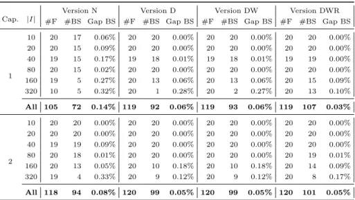
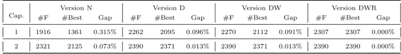
We propose four versions of the subproblem, which primarily depend on the degree of allowed modifications on the routes selected by the master problem. In the first version (denoted by N – No possible revision), we do not revise the charging decisions in the selected routes and we only check whether the CS capacity constraints are satisfied. In the second version (denoted by D – Delay), we allow delaying the starting time of each route (i.e., we postpone the departure of the EV from the depot) to satisfy the CS capacity constraints. We note that in versions N and D no increase in the total time of the solution is incurred. In the third version (denoted by DW – Delay+Waiting times), we

allow delaying the starting time of each route, and we also allow vehicles to wait for a charger if a CS is overcrowded by EVs. In DW, waiting times can only occur when a route stops several times for charging, since, when there is only one stop at a CS, delaying the starting time of the route is preferable, as this does not penalize the objective function. In the fourth version (denoted by DWR – Delay+Waiting times+Revision of charging amounts), we also revise the amount of energy charged at the CSs. If a route contains at least two stops at CSs, we may decide to charge more during the first stop in order to avoid waiting at the second stop before charging the EV. We note that this strategy may sometimes avoid detouring to one of the CSs visited in the original route.

We designed a branch-and-cut algorithm to efficiently solve the assembling problem while exploiting the decompo-sition discussed above. While solving the route selection problem, we dynamically solve the CS capacity management subproblem. More specifically, at each node of the branch-and-bound tree, we solve the subproblem for the current selection of routes. Depending on the version of the subproblem, we generate different cuts to discard infeasible route selections (see§4.2.3). For versions DW and DWR, we also add cuts to account for the underestimation of the increase in the total time to visit the customers.

We outline the general structure of the branch-and-cut method in Algorithm 3 (we focus on its most common used implementation based on interacting with the branch-and-bound procedure embedded into the MILP solver via callback routines). When provided as an input, we give to the solver the objective function value of a solution to the E-VRP-NL-C as a cutoff value (i.e., an upper bound on the value of the objective function of the master problem). Therefore, the solver only considers the solutions with an objective function value strictly less than this cutoff value. The solver returns the best solution assembled from a given pool of routes by the branch-and-cut algorithm. The component also returns a set Φ of improving solutions (compared to the initial solution s) computed throughout the algorithm. Whenever a selection of routes ¯x at an integer node of the branch-and-bound tree does not lead to the introduction of a cut after solving the capacity management subproblem CM P.p¯xq, we save it along with the updated charging decisions (delays,

waiting times, revision of charging amounts) to build a complete solution. Algorithm 3: The assembling procedure (focus on the implementation)

Input : a pool Ω of routes / a solution s (possibly equal to NULL) to the E-VRP-NL-C

Output: the best solution s˚_{computed by the branch-and-cut algorithm / a set Φ of improving solutions to the}

E-VRP-NL-C (in comparison with s) Procedure assemble(Ω,s):

‚ Build the MILP formulation rHC1s or rHC2s of the route selection problem from pool Ω(see§4.2.1 and §4.2.2) ‚ Define the callback function (function called at every node of the branch-and-bound tree) as procedure

SolveSubProblem(¯x)(see Algorithm 4)and associate to it a CPU time limit of τSP per call

‚ Give the model rHC.s, the callback function, the cutoff value f psq (objective function value of s) to the MILP solver and launch it with a CPU time limit equal to τ

‚ Retrieve the best solution s˚computed within the CPU time limit and the set Φ of improving solutions (compared to s)

return ps˚_{, Φq}

In the following subsections, we provide a detailed description of our four versions of the CS capacity management subproblem. We use the following notation. The binary parameter apr, iq is equal to one if and only if route r P Ω serves customer i P I. We define parameter tprq as the duration of a route r P Ω, obtained from the route generation component. We denote by OpΩq the set containing all the charging operations occurring in the routes belonging to Ω, and by OjpΩq Ď OpΩq all the charging operations occurring at CS j P F in these routes. We denote by Optruq the

list of charging operations occurring in route r. Let rpoq and jpoq be the route and the CS associated with a charging operation o. Let Spoq and dpoq be the starting time and duration of charging operation o in the route rpoq P Ω. For each route r P Ω, we assume that the operations in Optruq are sorted in non-decreasing order of their starting times. We denote by sucpoq the charging operation following o in route rpoq. If there does not exist any charging operation after o, we set sucpoq “ ´1. For every route r P Ω and for each charging operation o P Optruq we denote by t`_{poq the total}

time (driving and customer serving) spent in r by the EV between its departure from jpoq and its arrival at jpsucpoqq or at the depot if sucpoq “ ´1. For each operation o, we also introduce two parameters ESpoq and LSpoq representing its earliest and latest possible starting times. The values of these parameters depend on the different versions of the subproblem and they are specified in the following subsections.

4.2.1 N and D subproblem versions

To model the route selection problem, we introduce a binary variable xrequal to 1 if and only if route r P Ω is selected.

A MILP formulation of this problem is then the following classical set partitioning model: rHC1s minimizeÿ rPΩ tprqxr (43) subject to ÿ rPΩ apr, iqxr“ 1 i P I (44) xrP t0, 1u r P Ω. (45)

The objective (43) is to select a subset of routes from Ω that minimizes the total duration. Constraints (44) ensure that each customer is visited exactly once. Constraints (45) set the domains of the decision variables.

Let Ω1`p¯xq denote the set of routes with at least one charging operation resulting from a feasible solution ¯x to the

above problem, i.e., Ω1`p¯xq “ tr P Ω : ¯xr “ 1 ^ Optruq ‰ Hu. Note that the routes without mid-route charging do

not need to be considered when verifying the CS capacity constraints. We also define Ω1`p¯x, jq Ď Ω<sub>1</sub>`p¯xq as the set of

routes with a charging operation at j P F .

Version N In this version of the subproblem, the CS capacity management subproblem does not revise the charging operations scheduled in the selected routes. It only checks the feasibility of the charging operations with respect to the capacity constraints. We therefore set ESpoq “ LSpoq “ Spoq. Let CMP1p¯xq be this subproblem defined for the routes

that belong to Ω₁`p¯xq. It can be decomposed into |F | independent problems, one for every CS. To solve CMP1p¯xq,

for every CS j P F we apply a polynomial algorithm to check the existence of subsets of operations overloading the CS. Specifically, we call procedure CheckCapacityCut(OjpΩ1`p¯xqq, Cj) to check whether the capacity constraints are

satisfied according to the scheduled charging operations in OjpΩ1`p¯xqq. We refer the reader to Algorithm 7 in Appendix

D for the details of this procedure.

Version D The main drawback of version N is that it may discard promising routes. Indeed, in some cases simply delaying the starting time of some of the routes may allow their combination into a feasible solution to the problem. Note that shifting the start time of a route does not increase the objective function. In version D, we seek to resolve capacity violations by shifting starting times of the routes. Let CMP2p¯xq be this subproblem. In contrast to CMP1p¯xq, CMP2p¯xq

does not decompose into an independent problem for each CS. Let o be a charging operation. Its earliest starting time ESpoq is equal to Spoq since by construction the operations are left shifted in each route of the pool. The parameter LSpoq is computed by subtracting from Tmaxthe time needed to complete the route (considering the duration of the next charging

operations, the driving times, and no waiting times). Specifically, LSpoq “ Tmax´ř_o1_{POptrpoquq:Spo}1_qěSpoqpt`po1q ` dpo1qq.

We now define a continuous-time MILP formulation of CMP2p¯xq. Let the variable So define the starting time of

operation o P OpΩ1`p¯xqq. We model the capacity constraints using the flow-based formulation used in Section 3. For

each CS j P F , we consider two dummy operations o`j and o ´

j, and we define Cpoq :“ 1 for all o P OjpΩ1`p¯xqq and

Cpo`_jq :“ Cpo´_jq :“ Cj. We then introduce the continuous variable foo1 representing the quantity of resource (i.e.,

chargers) that is transferred from charging operation o to charging operation o1_{. We also define the sequential binary}

variable uoo1 taking the value of 1 if operation o is processed before operation o1. The MILP formulation of CMP2p¯xq

is as follows:

rCMP2p¯xqs minimize 0 (46)

subject to uoo1` uo1<sub>o</sub>ď 1 j P F, o, o1P OjpΩ1`p¯xqq : o ă o1 (47)

uoo2 ě uoo1` uo1o2´ 1 j P F, o, o1, o2P OjpΩ1`p¯xqq (48)

So1ě So` dpoquoo1` pLSpoq ´ ESpo1qqpuoo1´ 1q j P F, o, o1P OjpΩ1`p¯xqq (49)

Ssucpoq“ So` dpoq ` t`poq o P OpΩ1`p¯xqq : sucpoq ‰ ´1 (50)

ÿ o1_POjpΩ 1`p¯xqqYto ` ju fo1o “ 1 j P F, o P OjpΩ1`p¯xqq (51) ÿ o1<sub>POjpΩ</sub> 1`p¯xqqYto ` ju fo1o´ ÿ o1<sub>POjpΩ</sub> 1`p¯xqqYto ´ ju foo1 “ 0 j P F, o P OjpΩ1`p¯xqq (52)

ÿ oPOjpΩ1`p¯xqqYto ´ ju f<sub>o</sub>` j,o“ Cj j P F (53) ÿ oPOjpΩ1`p¯xqqYto ` ju f_o,o´ j “ Cj j P F (54)

foo1ď max`Cpoq, Cpo1q˘ uoo1 j P F, o, o1P OjpΩ1`p¯xqq (55)

ESpoq ď Soď LSpoq o P OpΩ1`p¯xqq (56)

foo1ě 0 j P F, po, o1q P`OjpΩ1`p¯xqq Y to`ju ˘ Y`OjpΩ1`p¯xqq Y to´ju ˘ (57) uoo1P t0, 1u j P F, o, o1P OjpΩ1`p¯xqq. (58)

CMP2p¯xq is a feasibility problem. Constraints (47) state that for two distinct operations o and o1, either o precedes o1,

o1_{precedes o, or o and o}1_{are processed in parallel (if there is more than one charger at the CS). Constraints (48) express}

the transitivity of the precedence relations. Constraints (49) are the disjunctive constraints on the operations related to the same CS. Each such constraint is active when uoo1 “ 1 and, in which case, it enforces the precedence relation

between charging operations o and o1_{. Note that no waiting times can occur before a charging operation. Constraints}

(50) enforce the precedence relation and the time lag between the charging operations occurring in the same route. Constraints (51) state that a charger has to be allocated to each charging operation. Constraints (52) ensure flow conservation. Constraints (53) and (54) define the value of the flow leaving the source and the flow entering the sink. Constraints (55) couple the flow variables with the sequence variables. Constraints (56) and (58) define the domains of the decision variables.

4.2.2 DW and DWR subproblem versions

In these versions of the subproblem, we allow a possible increase in the total duration of the routes. Indeed, introducing waiting times at CSs or revising the amount of charged energy may help resolve capacity violations, but such modifica-tions may extend routes due to the non-linearity of the charging funcmodifica-tions and the consideration of multiple charging technologies. Let θ be a non-negative variable estimating the added delay when solving the CS capacity management subproblem. A MILP formulation of the route selection problem (derived directly from rHC1s) follows:

rHC2s minimize ÿ

rPΩ

tprqxr` θ (59)

subject to (44), (45)

θ ě 0. (60)

Thereafter, we assume that we have a fixed selection Ω1`p¯xq of routes given by fixing the variables txrurPΩ to values

respecting the current constraints of the route selection problem.

Version DW In this version of the subproblem, we assume that EVs can wait at CSs if delaying the starting times of the routes is not sufficient to avoid capacity violations. Let CMP3p¯xq be the scheduling subproblem of the routes

Ω₁`p¯xq, which has the objective of minimising the addition of waiting times. The MILP formulation of CMP3p¯xq uses

the decision variables So, foo1, uoo1defined in CMP2p¯xq. We also introduce variable ∇othat represents the waiting time

incurred before the start of charging operation o P OpΩ1`p¯xqq. For every charging operation o, its earliest starting time

ESpoq is equal to Spoq and its latest starting time LSpoq is equal to Tmax´ř_o1_{POptrpoquq:Spo}1_qěSpoqpt`po1q ` dpo1qq. The

MILP formulation of CMP3p¯xq is as follows:

rCMP3p¯xqs minimize

ÿ

oPOpΩ_1`p¯xqq

∇o (61)

subject to (47) ´ (49), (51) ´ (58)

Ssucpoq“ So` dpoq ` t`poq ` ∇sucpoq o P OpΩ1`p¯xqq : sucpoq ‰ ´1 (62)

The objective (61) is to minimize the waiting time inserted in each route. Constraints (62) define the minimum time lag between the charging operations occurring in the same route. Constraints (63) define the domains of the waiting decision variables.

Version DWR In this version of the subproblem, in addition to the introduction of waiting times, resolving capacity violations at CSs can also be achieved by revising the amounts of energy charged at each CS in every route. We denote by CMP4p¯xq the subproblem in which we want to minimize the increase in the duration of the selected routes. Indeed,

revising the charging operations leads to an increase in time when the CSs in a route have different charging technologies or when the charging functions are non-linear. Note that if we substantially increase the charging amounts at a CS we may not need to stop at the subsequent CS in the route. We therefore need to account for the potential removal of stops at CSs.

We denote by e`_{poq the energy consumption of the EV between its departure from jpoq and its arrival at jpsucpoqq}

if sucpoq ‰ ´1. This takes into account the energy consumed to visit all the customers scheduled in the route between charging operations o and sucpoq or the depot. Since a charging operation can be skipped by charging more energy during the previous or next charging operations of the same route, we define rtpoq andrepoq as the driving time and energy saved if the EV does not detour to perform the charging operation o. We define Ω2`p¯xq as the subset of Ω1`p¯xq

that contains only the routes including at least two charging operations (i.e., Ω2`p¯xq “ tr P Ω<sub>1</sub>`p¯xq : |Optruq| ě 2u).

Our formulation of CMP4p¯xq draws upon formulation rCMP3p¯xqs. Aside from using decision variables defined in

the latter, rCMP4p¯xqs also uses the following decision variables for the operations in OpΩ2`p¯xqq. The variables t_o and

to are the scaled arrival and departure times, according to the charging function of CS jpoq. The binary variables

w_ok and wok are equal to 1 if and only if the SoC lies between qjpoq,k´1and qjpoq,k, with k P Bjpoqzt0u, upon starting

and finishing operation o, respectively. The continuous variables λok and λok are the coefficients associated with the

breakpoints pajpoq,k, qjpoq,kq of φjpoq upon starting and finishing operation o, respectively. The continuous variables y_o

and y_o represent the SoC of the EV upon starting and finishing charging operation o. The continuous variable ∆o

represents the duration of charging operation o.

For each route, we check whether it might be possible for a charging operation o to be skipped by considering that the EV leaves the previous CS (or depot) with a fully replenished battery. If this allows the EV to reach the next CS or to return to the depot without performing o, then we allow the EV not to detour to the corresponding CS. To this end, we introduce the binary variable zoequal to 1 if and only if the charging operation o is executed.

We also compute for every charging operation the time windows during which it must be scheduled. The earliest starting time ESpoq of a charging operation o is computed assuming that the EV skips (if the previous computation has shown it is possible) the previous charging operations (if any), and charges the maximum between the energy needed to recover the detour to the CS and the energy required to reach the next CS. To compute the latter, we consider that the SoC of the EV upon arriving at the CS is maximal (i.e., a full charge occurs at the previous CS). Then, we estimate the charging times assuming that the EV arrives with an empty battery. The latest starting time LSpoq of operation o is computed assuming that the EV returns to the depot at time Tmaxand assuming that the EV skips the next charging

operations (if possible).

The MILP formulation of CMP4p¯xq is as follows:

rCMP4p¯xqs minimize ÿ oPOpΩ<sub>1`</sub>p¯xqq ∇o` ÿ oPOpΩ<sub>2`</sub>p¯xqq `∆o´ dpoq ´ p1 ´ zoqrtpoq ˘ (64) subject to (47) ´ (48), (52) ´ (58), (63) y o“ ÿ kPB_jpoq λokqjpoqk o P OpΩ2`p¯xqq (65) to“ ÿ kPBjpoq λokajpoqk o P OpΩ2`p¯xqq (66) ÿ kPBjpoq λ_ok “ ÿ kPB_jpoqzt0u w_ok o P OpΩ2`p¯xqq (67) ÿ kPBjpoqzt0u w<sub>ok</sub>“ zo o P OpΩ2`p¯xqq (68) λ_o0ď wo1 o P OpΩ2`p¯xqq (69)

λ_okď wok` wo,k`1 o P OpΩ2`p¯xqq, k P Bjpoqzt0, bjpoqu (70)

λ_ob

jpoq ď wobjpoq o P OpΩ2`p¯xqq (71)

y_o“ ÿ kPB_jpoq λoqjpoqk o P OpΩ2`p¯xqq (72) to“ ÿ kPB<sub>jpoq</sub> λoajpoqk o P OpΩ2`p¯xqq (73) ÿ kPB_jpoq λok “ ÿ kPBjpoqzt0u wok o P OpΩ2`p¯xqq (74) ÿ kPB<sub>jpoq</sub>zt0u wok“ 1 o P OpΩ2`p¯xqq (75) λo0ď wo1 o P OpΩ2`p¯xqq (76)

λokď wok` wo,k`1 o P OpΩ2`p¯xqq, k P Bjpoqzt0, bjpoqu (77)

λob_jpoq ď wob_jpoq o P OpΩ2`p¯xqq (78)

∆o“ to´ to o P OpΩ2`p¯xqq (79)

∆oď ajpoq,bjpoqzo o P OpΩ2`p¯xqq (80)

y

ofirstprq“ qfirstprq r P Ω2`p¯xq (81)

y

sucpoq“ yo´ e `

poq `repoqp1 ´ zoq o P OpΩ2`p¯xqq : sucpoq ‰ ´1 (82)

yo´ e `

poq `repoqp1 ´ zoq ě 0 o P OpΩ2`p¯xqq : sucpoq “ ´1 (83)

So1 ě So` dpoquoo1` pLSpoq ´ ESpo1qqpuoo1´ 1q j P F, o, o1

P OjpΩ1`p¯xqzΩ<sub>2</sub>`p¯xqq (84)

So1 ě So` ∆o` pLSpoq ´ ESpo1qqpuoo1´ 1q j P F, o, o1P OjpΩ2`p¯xqq (85)

Ssucpoq“ So` dpoq ` t`poq ` ∇sucpoq o P OpΩ1`p¯xqzΩ2`p¯xqq : sucpoq ‰ ´1 (86)

Ssucpoq“ So` ∆o` t`poq ´ rtpoqp1 ´ zoq ` ∇sucpoq o P OpΩ2`p¯xqq : sucpoq ‰ ´1 (87)

So` ∆o` t`poq ´ rtpoqp1 ´ zoq ď Tmax o P OpΩ2`p¯xqq : sucpoq “ ´1 (88)

ÿ o1_PO jpoqpΩ1`p¯xqqYto ` jpoqu fo1o“ 1 o P OpΩ1`p¯xqzΩ<sub>2</sub>`p¯xqq (89) ÿ o1_PO jpoqpΩ1`p¯xqqYto ` jpoqu fo1_o“ zo o P OpΩ2`p¯xqq (90) zoP t0, 1u, ∆oě 0, 0 ď y o ď Q, 0 ď yoď Q o P OpΩ2`p¯xqq (91)

w_ok, wokP t0, 1u, o P OpΩ2`p¯xqq, k P Bjpoqzt0u (92)

λ_ok, λokP t0, 1u o P OpΩ2`p¯xqq, k P Bjpoq. (93)

The objective (64) is to minimize the total additional time inserted in each route. Constraints (65)–(79) model the piecewise linear charging functions. Constraints (80) impose a duration equal to 0 for each charging operation that is not executed anymore. For each route r P Ω2`p¯xq, constraints (81) define the SoC qfirstprq of the EV upon starting

its first charging operation (denoted ofirstprq). Constraints (82) couple the SoC of the EV after finishing a charging

operation with its SoC when starting the next charging operation occurring in the route. Note that if zo is equal to

0, then the SoC y

o “ yo still takes into account the energy consumed to detour to CS jpoq. The energy saved by not

stopping at this CS is subtracted when computing the SoC at the beginning of the next operation of the route or at the arrival at the depot (see (83)). For each route, constraints (83) force the corresponding EV to have enough SoC at the end of the last charging operation to reach the depot. Constraints (84) and (85) are the disjunctive constraints on the operations related to the same CS. Constraints (86) and (87) define a minimum time lag between the charging operations occurring in the same route. Note that if zo is equal to 0, then the starting time So still takes into account

the detour to CS jpoq. The time saved by not stopping at this CS is subtracted during the computation of the departure time for the next operation of the route. Constraints (88) limit the route duration. Constraints (89) and (90) assign a charger to each operation that is executed. Constraints (91)–(93) define the domains of the new decision variables.